Structure of the oceanic lithosphere and upper mantle north of the Gloria Fault in the eastern mid-Atlantic
by receiver function analysis
Katrin Hannemann1 , Frank Krüger2, Torsten Dahm2,3, and Dietrich Lange1
1GEOMAR-Helmholtz Centre for Ocean Research Kiel, Kiel, Germany,2Institute of Earth and Environmental Science, University of Potsdam, Potsdam, Germany,3Section 2.1, Physics of Earthquakes and Volcanoes, GFZ Potsdam, Potsdam, Germany
Abstract
Receiver functions (RF) have been used for several decades to study structures beneath seismic stations. Although most available stations are deployed on shore, the number of ocean bottom station (OBS) experiments has increased in recent years. Almost all OBSs have to deal with higher noise levels and a limited deployment time (∼1 year), resulting in a small number of usable records of teleseismic earthquakes.Here we use OBSs deployed as midaperture array in the deep ocean (4.5–5.5 km water depth) of the eastern mid-Atlantic. We use evaluation criteria for OBS data and beamforming to enhance the quality of the RFs.
Although some stations show reverberations caused by sedimentary cover, we are able to identify the Moho signal, indicating a normal thickness (5–8 km) of oceanic crust. Observations at single stations with thin sediments (300–400 m) indicate that a probable sharp lithosphere-asthenosphere boundary (LAB) might exist at a depth of∼70–80 km which is in line with LAB depth estimates for similar lithospheric ages in the Pacific. The mantle discontinuities at∼410 km and∼660 km are clearly identifiable. Their delay times are in agreement with PREM. Overall the usage of beam-formed earthquake recordings for OBS RF analysis is an excellent way to increase the signal quality and the number of usable events.
1. Introduction
More than 70% of the Earth is covered by oceans, and the majority of the oceanic crust is not affected by recent volcanic or tectonic activities like mid-ocean ridges, subduction zones, or hot spots. ThePwave velocity-depth structure of the oceanic crust and uppermost mantle has been characterized by active geophysical exper- iments [e.g.,White et al., 1992]. Deeper structures in the oceanic lithosphere and upper mantle are studied using broadband ocean bottom stations (OBSs) [e.g.,Suetsugu and Shiobara, 2014]. In recent years, several passive large-scale experiments with OBSs have been conducted [e.g.,Friederich and Meier, 2008;Barruol and Sigloch, 2013;Gao and Schwartz, 2015;Lin et al., 2016;Ryberg et al., 2017]. Nevertheless, most of the OBS studies are located at mid-ocean ridges [e.g.,Shen et al., 1998a;Tilmann and Dahm, 2008;Jokat et al., 2012;Grevemeyer et al., 2013;Hermann and Jokat, 2013;Schlindwein et al., 2013, 2015], hot spots [e.g.,Suetsugu et al., 2007;Barruol and Sigloch, 2013;Davy et al., 2014;Geissler et al., 2016;Ryberg et al., 2017], subduction zones [e.g.,Suetsugu et al., 2010;Kopp et al., 2011;Laigle et al., 2013;Ruiz et al., 2013;Grevemeyer et al., 2015;Janiszewski and Abers, 2015] or the transition from continental crust to oceanic crust [e.g.,Czuba et al., 2011;Grad et al., 2012;Libak et al., 2012;Suckro et al., 2012;Monna et al., 2013;Altenbernd et al., 2014;Kalberg and Gohl, 2014], and are thus not representative of undisturbed oceanic crust and mantle.
Most of our knowledge of the oceanic mantle is based on global surface wave tomography [e.g.,Romanowicz, 2009], with rather good path coverage in the oceans but low resolution for sharp discontinuities. Furthermore, studies using land based stations at teleseismic distances have been conducted to analyze underside reflec- tions to resolve oceanic mantle structures (PP and SS precursors) [Gossler and Kind, 1996;Gu et al., 1998;
Flanagan and Shearer, 1998;Gu and Dziewonski, 2002;Deuss et al., 2013;Saki et al., 2015]. Both methods lack spatial resolution. On the other hand, receiver function (RF) analysis provides a strong tool to image discon- tinuities in the lithosphere and the upper mantle down to the transition zone with high lateral resolution [e.g.,Vinnik, 1977;Langston, 1979]. So far only a limited number of receiver function (RF) studies of undis- turbed oceanic lithosphere have been conducted using 500 m deep borehole stations and OBSs [Suetsugu et al., 2005;Kawakatsu et al., 2009;Olugboji et al., 2016].
RESEARCH ARTICLE
10.1002/2016JB013582
Key Points:
• First evidence of a normal mantle transition zone in the mid-Atlantic from RFs in the deep ocean
• Improve signal quality of OBS receiver functions (RFs) by quantitative evaluation and beamforming
• Body wave imaging of discontinuities in mid-oceanic lithosphere and upper mantle using OBS data
Correspondence to:
K. Hannemann, khannemann@geomar.de
Citation:
Hannemann, K., F. Krüger, T. Dahm, and D. Lange (2017), Structure of the oceanic lithosphere and upper mantle north of the Gloria Fault in the eastern mid-Atlantic by receiver function analysis,J. Geophys. Res. Solid Earth,122, 7927–7950, doi:10.1002/2016JB013582.
Received 22 SEP 2016 Accepted 11 AUG 2017
Accepted article online 15 AUG 2017 Published online 13 OCT 2017
©2017. American Geophysical Union.
All Rights Reserved.
This study focuses on OBS RFs in the eastern mid-Atlantic in the vicinity of the Eurasian-African plate boundary, in which—to our knowledge—no OBS RF study has previously been done. We target major discontinu- ities within the oceanic lithosphere and mantle. The Mohoroviˇci´c discontinuity (Moho) marks the boundary between oceanic crust and mantle and is expected in depths between 5 and 8 km [e.g.,White et al., 1992].
Thickened or thinned oceanic crust may be related to overthrusting, underplating, or basin formation. The RF phase of the Moho arrives only 1 or 2 s after the dominantPphase [e.g.,Kawakatsu et al., 2009] and therefore requires high-frequency data [Audet, 2016], and a good signal-to-noise ratio (SNR). Furthermore, it is often masked by sediment reverberations which hamper a direct interpretation of the Moho signal [Audet, 2016;
Kawakatsu and Abe, 2016].
The lithosphere-asthenosphere boundary (LAB) beneath the oceans is often imaged using surface waves [e.g.,Romanowicz, 2009;Takeo et al., 2013, 2016;Lin et al., 2016], SS waveforms [e.g.,Rychert et al., 2012], RFs employing land stations [e.g.,Li et al., 2000;Kumar and Kawakatsu, 2011], or OBSs [e.g.,Kawakatsu et al., 2009;
Olugboji et al., 2016]. Most of the discussed models of the LAB [Kawakatsu et al., 2009;Fischer et al., 2010;
Olugboji et al., 2013] include thermal control, changes in rheology, dehydration, anisotropy, or partial melt.
Experiments with polycrystalline materials [Takei et al., 2014;Yamauchi and Takei, 2016] at subsolidus temper- atures indicate that solid state mechanism such as diffusionally accommodated grain boundary sliding play an important role forSwave velocity decrease with rising temperature in the oceanic lithosphere [Yamauchi and Takei, 2016, Figure 20]. Besides the depth of the LAB, the sharpness of the discontinuity is of interest.
A relatively smooth transition would be expected if the position of the LAB is purely thermally controlled [Olugboji et al., 2013] and a sharp boundary if it is controlled by composition (e.g., abrupt change in water content [Karato and Jung, 1998]). Both of these cases mark end-member models, and a variety of interme- diate models may be possible (e.g., a gradual change in the water content leading to a smooth transition).
For example, a land-basedSwave RF study of oceanic lithosphere in subduction zones [Kumar and Kawakatsu, 2011] supports the model of thermal control, but the observed scatter in the observations indicates addi- tional controlling factors. Observations of the oceanic LAB indicate a diffuse age-dependent boundary in young oceans and a sharp age-independent LAB at∼70 km in old oceans [e.g.,Fischer et al., 2010;Karato, 2012;Olugboji et al., 2013]. A subsolidus model which assumes grain boundary sliding [Karato, 2012;Olugboji et al., 2013] predicts a transition from an age-dependent diffuse LAB roughly following the 1300 K isotherm in young oceans, to a sharp discontinuity at constant depth in old oceans. The age at which this transition happens, depends on the thermal model used for the modeling and lies between 40–80 Ma [Karato, 2012] or between 55–75 Ma [Olugboji et al., 2013].
The Lehmann discontinuity is assumed to mark the lower boundary of the asthenosphere [e.g.,Lehmann, 1961;Dziewonski and Anderson, 1981;Deuss et al., 2013]. It is located at around 220 km depth, and its cause is still debated [Karato, 1992;Deuss and Woodhouse, 2004]. Only a few RF [Shen et al., 1998a] and SS precursor observations [Deuss and Woodhouse, 2002] exist of the oceanic Lehmann discontinuity.
The three global mantle discontinuities at approximately 410 km, 520 km, and 660 km depth (referred to as
“410,” “520”, and “660,” respectively) are associated with phase transitions in olivine or the aluminum phases (e.g., garnet) of the mantle [e.g.,Agee, 1998;Helffrich, 2000;Deuss et al., 2013]. In the ocean, the mantle tran- sition zone (MTZ), defined by the 410 and the 660, has mostly been studied by using PP and SS precursors [Gossler and Kind, 1996;Gu et al., 1998;Flanagan and Shearer, 1998;Gu and Dziewonski, 2002;Deuss et al., 2013;
Saki et al., 2015]. There are also some global RF studies of the MTZ [Chevrot et al., 1999;Lawrence and Shearer, 2006;Tauzin et al., 2008] and local studies focusing on the MTZ using OBS data [Shen et al., 1998a;Gilbert et al., 2001;Suetsugu et al., 2005, 2007, 2010]. Some global studies of SS precursors suggest a thinner MTZ beneath the oceans than below the continents [Gossler and Kind, 1996;Gu et al., 1998;Gu and Dziewonski, 2002]; however,Flanagan and Shearer[1998] (SS precursors) andChevrot et al.[1999] (RF) could not observe such a correlation. The lack of correlation is also confirmed by local studies [Shen et al., 1998a, 1998b;Silveira et al., 2010].
Here we use data from 11 OBSs located in the eastern mid-Atlantic approximately 100 km North of the Gloria Fault (Figure 1b) to investigate the structure of the oceanic crust and upper mantle using array techniques (e.g., “delay and sum” beamforming [Rost and Thomas, 2002]) and receiver functions. OBS data are usually characterized by a small amount of good-quality events within a short recording period of the deployed instruments (∼1 year) [Webb, 1998]. One of the main reasons is the often low signal-to-noise ratio (SNR) at ocean bottom stations [Webb, 1998;Dahm et al., 2006], especially in the horizontal components. There have
Figure 1.(a) Azimuthal equidistant plot of events used for RF analysis indicated as filled yellow circles (P and PKP single-station RFs) and as open orange circles (P and PKP beam RFs). The event details are listed in Table C1 (in the Appendix). (b) The top map shows the array configuration for the OBS. The color scale shows the water depth (EMEPC, Task Group for the Extension of the Continental Shelf ). The white dashed lines indicate the distance to the Gloria Fault.
The red triangle marks station D05 which has two clamped seismometer components. The black and white map shows the location of the OBS array within the eastern mid-Atlantic and the dashed line indicates the Eurasian-African plate boundary (Gloria Fault) [Bird, 2003].
been different strategies to increase the number of usable events: either by reinstalling the OBS at the same site (e.g., Cascadia Initiative) [Janiszewski and Abers, 2015] or recently by using array techniques [Thomas and Laske, 2015]. The latter is known to increase the SNR of an event by coherent stacking of the observed sig- nals [Rost and Thomas, 2002]. It uses the event’s azimuth and the slowness of the considered phase for the estimation of time delays between the stations which are then removed before stacking the single station recordings (beamforming) (for further details, seeRost and Thomas[2002]). The experiment presented here is designed in such a way that the stations form a midaperture array with interstation distances of 10–20 km and a maximum aperture of 75 km (Figure 1b). This design allows us to stack all stations to enhance phases originating from the deeper parts of the upper mantle. Additionally, we employ a quality control by using evaluation criteria such as relative spike position within the deconvolution time window and search for an optimal deconvolution length to improve the SNR of each RF. Furthermore, we analyze the RFs from single OBSs, stacks of all stations and beams in different frequency bands and compare amplitudes and delay times of the RFs with synthetic data.
2. Data
We use recordings of 11 OBSs that were installed in the deep sea (4.5–5.5 km water depth) of the eastern mid-Atlantic in 2011 (Figure 1b). These stations are equipped with three-component broadband seismome- ters (Guralp CMG-40T, 60 s—50 Hz) and hydrophones (HighTechInc HTI-04-PCA/ULF, 100 s—8 kHz, flat instrument response down to 5 s, at D08 down to 2 s) and recorded 100 Hz data. To obtain an accurate clock drift, we use ambient noise cross correlation and compare it to the drift calculated from the synchronization with GPS to reveal static time offsets [Hannemann et al., 2014]. Subsequently, we use the pyrocko toolbox (emolch.github.io/pyrocko) to apply a time correction by inserting and deleting samples. A twelfth station (D05) has not been used for the analysis because of two clamped seismometer components.
For the free fall OBSs used in this study, the orientation of the vertical component is aligned by a gimbaling system [Stähler et al., 2016]. Since for the OBS data the orientation of the horizontal components is unknown,
we testPphase polarization and Rayleigh and Love waves [Thorwart, 2006;Stachnik et al., 2012;Sumy et al., 2015] to align the horizontal components to the north and east (see Appendix A for details).
We use, in the following, the results of thePphase for the rotation of the horizontal traces, because we find from a frequency-wave number analysis with a moving time window using the vertical traces [Rost and Thomas, 2002] that the estimated back azimuths of thePphases are more precise than those of the Rayleigh phases. They show on average a smaller deviation from the expected back azimuths [see alsoThorwart, 2006].
For the RF calculation, we examine all events that have a body wave detection in our frequency-wave number detector with values ofPbetween∼30∘and 90∘epicentral distance,Pdiffbetween∼90∘and 110∘epicentral distance and PKPdfbetween∼140∘and 160∘epicentral distance. The events finally used (single: 25, beams:
37, see Tables C1 and C2 in the Appendix) are chosen based on the evaluation criteria described below.
3. Methods
When the up-going compressional wave (Pwave) is incident on an interface within the Earth, its upward propagating energy is partitioned into aPwave and a vertical polarized shear wave (SVwave). The latter is also referred to asP-to-S(Ps) wave conversion and is a secondary phase which arrives later than the direct Pphase (i.e., the refractedPwaves). The amplitudes of thePsconversions are typically several tens of times smaller than those of the directPphase, depending on theSwave velocity change at the discontinuity and the incidence angle [e.g.,Chevrot et al., 1999;Julià, 2007]. The relativePsamplitudes can be calculated from the ratio of the refraction coefficientṔṔxandṔ́Sxfor whichxindicates the depth of the discontinuity (seeAki and Richards[2002] for definition of acute accents). In addition to the problem of small relative amplitudes, the identification ofPsphases is often obscured by ambient noise and multiple reflections beneath the receiver.
Therefore, specific deconvolution and stacking methods were developed to enhance the signal-to-noise ratio (SNR) of the weakPsphase [Vinnik, 1977;Langston, 1979].
We calculate RFs in the vertical-radial coordinate system, ZRT (Z = vertical, R = horizontal radial, T = horizontal transversal) [e.g.,Hannemann et al., 2016]. For the rotation into ZRT, we use the theoretical azimuth obtained using the station position and the hypocenter of the corresponding earthquake (see Table C1 in the Appendix). ThePwave signal on the Z component is used to determine a time domain Wiener filter [e.g.,Kind et al., 1995] which transforms the rather complexPwave signal into a band-limited spike signal. The filter is then applied to the R component to obtain the ZR RF.
For the estimation of the Wiener filter, we use the built-in function “spiking” of Seismic Handler [Berkhout, 1977;Stammler, 1993] which is able to calculate an optimum lag spiking filter [Robinson and Treitel, 1980;
Yilmaz, 2008]. This function offers the possibility to use either the centroid of the signal,tc(center of mass, equation (1)), as the spike position or a user-specified spike position. In this study, we use the centroid of the signal,tc, as spike position, which is similar to the effective wavelet length as proposed byBerkhout[1977]:
tc=
∑N i=1i⋅||ai||
∑N
i=1||ai|| . (1)
The centroid of the signal,tc, is calculated for a deconvolution time window containingNamplitude samples using the sample number,i, and the amplitude,ai, of theith sample.
The inversion to determine the Wiener filter (inverse filter) works best for minimum phase signals [e.g., Scherbaum, 2001]. AsPwave signals are usually mixed phase signals, we stabilize the inversion matrix with a damping factor (0.01). The resulting RF shows several spikes representing converted phases and their multi- ples from different interfaces/discontinuities. The spikes of the secondary phases should be separated from the spike of the direct phase [Vinnik, 1977;Langston, 1979]. The amplitudes and delay times of the spikes of the secondary phases constrain theSwave velocity changes, their multiples the impedance contrast, and both the depths of the interfaces under investigation [e.g.,Julià, 2007]. The deconvolution removes the source time function from the RFs, so that RFs from different events can be stacked after the traces have been stretched to represent time functions on a common ray path. For this distance move-out correction [Yuan et al., 1997], we use a reference distance of 67∘and a global velocity model (oceanic PREM) [Dziewonski and Anderson, 1981].
The determination of RFs at OBSs may be influenced by water multiples [e.g.,Thorwart and Dahm, 2005] or noise (tilt or water wave compliance) [e.g.,Bell et al., 2015], which can be corrected on the vertical component
by using hydrophone data [e.g.,Thorwart and Dahm, 2005;Bell et al., 2015] or the horizontal components [e.g.,Bell et al., 2015]. We do not observe water multiples in our teleseismic recordings, and therefore, we do not apply any correction for them. Furthermore, the water wave compliance is only present at very low frequencies (∼100 s) in 4.5–5.5 km water depth [e.g.,Crawford et al., 1998;Bell et al., 2015]. We avoid this frequency band by high-pass filtering the RFs. The tilt noise cannot be excluded in our case and might influ- ence the RFs at periods longer than∼10 s. Tilting (e.g., movement of the OBS frame by currents) [Webb, 1998;
Crawford et al., 1998;Bell et al., 2015] has a higher influence on the horizontal components than on the ver- ticals and a correction of the vertical component [e.g.,Bell et al., 2015] would probably lead to rather similar results for the estimated RFs [e.g.,Janiszewski and Abers, 2015]. We therefore do not remove the tilt noise from the vertical component.
We find that the SNR of a RF is mainly determined by the quality of the earthquake recording and the length of the deconvolution time window used for the determination of the Wiener filter. To obtain RFs with sufficient SNR, we follow two approaches: (1) increase the SNR of earthquake recordings by employing “delay and sum”
beamforming [Rost and Thomas, 2002] using either the plain recordings, or normalize the recordings to the root-mean-square (rms) amplitude of the noise (−200 s to−100 s beforePonset) on a single component to optimize destructive interference of noise amplitudes, and (2) introduce a quality control which employs a set of evaluation criteria to select a subset of deconvolution lengths for single-station recordings and beams.
A beamforming approach using OBS data is not common, and to our knowledge, our study is the first to apply this technique before the calculation of OBS RFs. We employ the normalization of the earthquake recordings to the rms amplitude of the noise on the Z component to improve the signal used for the deconvolution and on the R component to suppress the noise on the horizontal components.
To determine whether the chosen time window contains a mainly minimum phase signal or mainly noise, we choose as first evaluation criterion the spike position,trel, relative to the deconvolution time window,tdec:
trel=tc−tdec
2
tdec . (2)
In the case of a mainly minimum phase signal, the spike position is located within the first half of the decon- volution time window (tc<tdec2 ⇒trel<0). On the other hand, if the time window contains mainly noise, the spike position is in the middle of the deconvolution time window (tc≈tdec
2 ⇒trel≈0).
The success of the deconvolution is estimated by the SNR of the Z component of the RF (SNRZ/Z), which is the second evaluation criterion used. It is determined by estimating the ratio of the squared rms amplitudes in the signal time window (−10 s to 10 s relative toPspike) and noise time window (−55 s to−25 s before Pspike) on the Z component.
In order to quantify the success of resolving upper mantle discontinuities, the third and last evaluation crite- rion is the ratio of the squared rms amplitudes of the signal time window on the Z component of the RF and the noise time window on the R component of the RF (SNRZ/R). We compare this to the theoretical ratios of the refraction coefficientsṔ́́P410
PŚ410 andṔ́́P660
PŚ660 assuming PREM velocities [Dziewonski and Anderson, 1981]. We test different deconvolution time window lengths,tdec, starting with 30 s and increasing the length in 5 s steps to a time window length which approximately equals the time difference between thePonset and thePP phase arrival. The deconvolution length for each single event recording and beam is chosen by the following four steps:
1.trel<0for mainly minimum phase signals (Figures 2a and 3a);
2. SNRZ/Z≳10for a good deconvolution (Figures 2b and 3b);
3. SNRZ/R≳ṔṔ́́PS660
660
and/or SNRZ/R≳ṔṔ́́PS410
410
for resolving upper mantle discontinuities (Figures 2c and 3c); and 4. manual revision of remaining RFs (Figures 2d and 3d).
The fourth step (manual revision) is required to exclude RFs which are influenced by high-frequency noise or ringing. These disturbed RFs are often hard to distinguish from undisturbed RFs with the simple evaluation criteria employed here.
We observe a small time shift in the first peak on the R component (Figure 2d) that can be explained by the influence of a sedimentary cover [Sheehan et al., 1995]. We calculated the mean preevent noise spectra andPwave spectra of all used events (Tables C1 and C2) using the ZRT components of the single stations
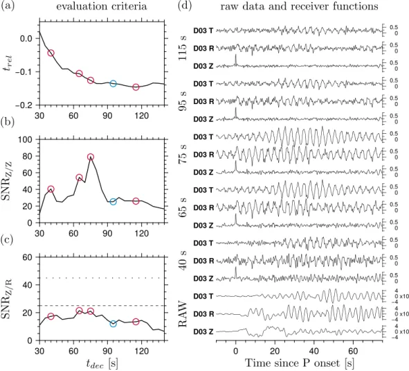
Figure 2.Example of the evaluation criteria shown against deconvolution time window length,tdec, and preselected deconvolution time window lengths for station D03 and event #30 (Table C1 in the Appendix). The circles mark the values for the RFs presented in Figure 2d. The blue circle indicates the final chosen deconvolution length (95 s).
(a) Relative spike position,trel, estimated with equation (2). (b) The SNR on the Z component. (c) The ratio of the signal time window on Z and the noise time window on R. For guidance the ratios of the refraction coefficients of the refracted PandSVwaves at the 410 (PṔ́́Ṕ410
S410, dotted line) and the 660 (ṔṔ́́P660
S660, dashed line) are indicated. (d) The unfiltered raw data (in counts) and the RFs (normed toPspike on Z) for the different preselected deconvolution lengths (circles in Figures 2a–2c).
and the beams without normalization (Figure B1 in the appendix). The spectra show that there is often a change in spectral characteristics between preevent noise spectra andPwave spectra. Furthermore, there is evidence for sedimentary reverberations at some stations (D01–D06). Moreover, a probabilistic power spectral density analysis (PPSD) [McNamara, 2004] reveals a resonance-like effect on all three seismometer components of each station [Hannemann et al., 2016]. These effects are also visible in the raw data in Figure 2d and are probably related to signal and ambient noise-induced reverberations in the sedimentary cover at each station [Hannemann et al., 2016]. The interpretation of RFs can be hampered by the presence of such rever- berations and must therefore be done carefully [Audet, 2016;Kawakatsu and Abe, 2016]. Furthermore, the ZRT coordinates are preferred for the calculation of RFs at OBSs, as the usage of the ray-oriented coordinate sys- tem (LQT) may lead to a large amplitude at 0 s on the Q component of the LQ RFs in the presence of sediment reverberations [e.g.,Olugboji et al., 2016], which cannot be modeled by using a 1-D velocity-depth model.
Using the events from Tables C1 and C2 (in the Appendix), we find that beamforming improves—as expected—the SNRZ/Zand the SNRZ/R(Figure 3) and that this effect can be enhanced by a normalization of the individual traces before stacking (red and blue lines compared to yellow lines in Figures 3b and 3c). We get the highest SNRZ/Zvalues of the tested normalizations for the RFs of the beams with a prenormalization
Figure 3.Same as Figure 2 but for traces resulting from beamforming for event #30 (Table C1 in the Appendix) and different normalization of single-station recordings (PLN, no prenormalization (yellow), ZNR, prenormalized to rms amplitude of noise on Z (red), RNR, prenormalized to rms amplitude of noise on R (blue)). The gray lines show the evaluation criteria for station D03 (Figures 2a–2c). The circles in Figures 3a–3c indicate the values for a deconvolution length of 110 s as is used for the RFs in Figure 3d.
to the rms amplitude of the noise on the Z component (ZNR). On the other hand, the highest SNRZ/Rof the tested normalizations is observed for the RFs of the beams with a prenormalization to the rms amplitude of the noise on the R component (RNR). We therefore present only the ZR RFs for the beams with prenormaliza- tion to the noise on either the Z or R component (ZNR or RNR) in the following analysis. Furthermore, we find that in our study 2–4 times more events are usable for the RF analysis utilizing beams than in the case of a single OBS (Table C2 in the Appendix).
For the RF analysis, we perform a bootstrap [Efron and Tibshirani, 1986] to estimate the uncertainties of the picked delay times and the confidence levels of the RF amplitudes. For this purpose, we randomly choose the RFs before stacking the distance move-out corrected traces and repeat this procedure for 300 trials [e.g.,Suetsugu et al., 2010]. Furthermore, we use the amplitudesbi(t)at timetof the total number of boot- strapped traces (M=300) to calculate the standard error𝜎(t)[Deuss, 2009] of the amplitude of the stacked RFd(t)at timet:
𝜎(t) =
√ ∑M i=1
[d(t) −bi(t)]2
M(M−1) . (3)
We indicate the 95% confidence levels of the RFs by plotting twice the standard error𝜎(t)for the presented RF stacks. For a better visibility, we shade the areas beneath positive amplitudes in blue for which the lower confidence level is larger than zero and the areas above negative amplitudes in red for which the upper
Figure 4.(a) Band-pass-filtered ZR receiver functions (0.5 s to 60 s). All traces have been normalized to thePspike on the Z component of the RFs. The colored areas show where the 95% confidence level is above zero (blue) and below zero (red) for the corresponding stations, all stations (SUM), beam-formed traces prenormalized to rms amplitude of noise on Z (ZNR) and on R (RNR). Markers indicate the positions of the Moho signal with two standard deviations estimated by picking 300 bootstrapped ZR RFs. Markers with a question mark show low confidence delay time picks.
At stations D01, D07, and D10, we identify possible sediment phases. (b) Comparison of OBS RF (red, same order as in Figure 4a to synthetic RFs calculated for models obtained byPwave polarization analysis (black) [Hannemann et al., 2016], and for a model with 7 km thick oceanic crust (gray). The normalized beams have not been modeled; instead, the synthetics for the all stations stack (SUM) are shown. The solid lines mark the theoretical delay times of the sediment layer and the dotted lines of the Moho. The colors represent thePs(black),PpPs(blue), andPpSs(orange) phase. For the single stations, the theoretical delay times for the corresponding models byHannemann et al.[2016] are used, and in the case of all stations and the normalized beams the theoretical Moho delay times for a 7 km thick oceanic crust are shown. The number in front of each trace indicates the number of events which contributed to the RF stacks.
confidence level is smaller than zero (e.g., Figure 4a). Since the data in our OBS network have a higher noise level compared to most land stations, such a rigorous analysis and visualization of uncertainties is very helpful for the interpretation.
4. Results and Discussion
In this study, we determine the time difference between the converted (Ps) and the direct (P) phase (hereafter referred to as the delay time) on move-out corrected, stacked receiver functions (RFs) of several earthquakes.
Table 1.Delay Times for Selected Stations and Stack of All Stations for the Mohoa
Station D01 D06 D07 D10 D11 SUM
tMoho(s) (1.18±0.08) (0.70±0.02) 0.74±0.03 (1.14±0.09) (0.85±0.05) 0.69±0.05
aThe delay times are estimated by picking the corresponding phase on 300 stacked traces which are formed by bootstrapping the contributing ZR RF traces for each plain stack. The times are given with an error of 1 standard deviation. Estimates in brackets represent low confidence delay time picks as indicated in Figure 4a.
In the following, we discuss the observedPsphases from different depth levels and discontinuities in the crust and upper mantle.
4.1. Structure of the Oceanic Crust
In Figure 4a, we show the band-pass filtered (0.5 s to 60 s) ZR RFs for the single OBSs (D01–D12), the stack of all stations (SUM), and the stack of the beam-formed traces (ZNR and RNR). In addition, we present in Figure 4b the comparison with synthetic RFs calculated for velocity-depth models obtained byPwave polarization anal- ysis (black) [Hannemann et al., 2016] which consist of a sedimentary, a crustal and an uppermost mantle layer over PREM, and a simple model without a sediment layer and an oceanic crustal thickness of 7 km (gray).
As previously stated, the time shift of the first peak on the RFs indicates the presence of a sedimentary layer and is also visible in the mismatch between the OBS RFs and the synthetics obtained for the 7 km thick oceanic crust. The presence of a sedimentary cover as estimated byHannemann et al.[2016] leads to a complex inter- ference pattern of sediment and Moho phases and multiples in the first seconds of the RFs (compare the black curves in Figure 4b). This biasing effect of a sedimentary cover often restricts the direct interpretation of OBS RFs [Audet, 2016], as discussed byKawakatsu and Abe[2016].
In a comparison with the synthetic data (Figure 4b), we identify a positive early arrival on the ZR RFs of the stations D01, D07, and D10, and probably D08 which may be related to the sediment layer. The delay times at D01 (∼0.3 s) and D07 (∼0.1 s) match well with the theoretical delay times of the models obtained by Hannemann et al.[2016] (D01: 0.28 s, D07: 0.09 s). At station D10, the first positive amplitude arrives slightly later (∼0.2 s) than predicted by the synthetic model (0.09 s) [Hannemann et al., 2016]. This may be caused by the poorly resolved sediment layer in the model for station D10 [Hannemann et al., 2016]. At station D08, the synthetic RF suggests that the first peak is likely a mixture of several phases. In general, mismatches between the synthetics calculated with the sediment models obtained byHannemann et al.[2016] and the OBS data are found particularly for those stations at which the sediment model is based on only fewPwave recordings, i.e., in the case of stations D09 and D12.
For the identification of the Moho and the determination of its robustness, we use the information provided by the comparison of the ZR RFs with the synthetic data (Figure 4b), and the 95% confidence level. In conclusion, we find one single station within the array (D07) at which we are confident about the identified Moho (Figure 4 and Table 1). First of all, the lower confidence level identifies this peak as being robust for all bootstrapped traces. Second, the OBS RFs and the synthetic RFs have a similar appearance which indicates low influence of noise on the RFs. There is some evidence for the presence of a Moho-related signal at other single stations (D01, D06, D10, and D11, Table 1), but the comparison with the synthetic data and the estimated confidence levels indicate that these are biased by the interference with sediment related signals.
Furthermore, the ZR RF stacks of all stations provides an estimate for an average Moho delay time (0.68 s, Figure 4a and Table 1). Although the beam-formed traces ZNR and RNR show comparable amplitudes to the stack of all stations (SUM), we cannot clearly identify the Moho signal on these beam traces. This is proba- bly related to the effect of the interference of the reverberations originating from the different sedimentary models at the individual stations in the beam-formed traces which leads to the observed broad peak in the RF beams.
We estimate theoreticalPsdelay times for depth intervals of 2 km using the PREM velocity model [Dziewonski and Anderson, 1981] and a slowness of 6.4 s/∘, which corresponds to a distance of 67∘, which was also used for the move-out correction. Based on these values, we estimate pseudodepths using the obtained Moho delay times (Table 1). This results in depths of 4.8–5.1 km for station D07 and the stack of all stations (SUM). This crustal thickness is less than the expected values for oceanic crust [e.g.,White et al., 1992;Laske et al., 2013] and slightly less than the values obtained byHannemann et al.[2016]. In addition, we marked
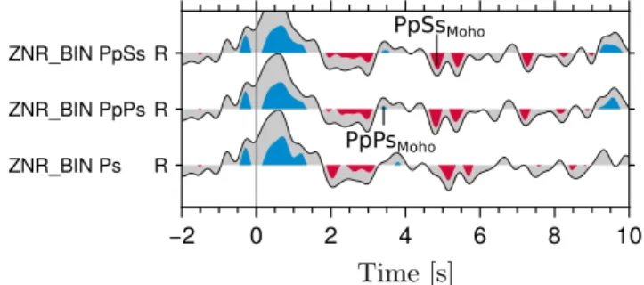
Figure 5.Move-out corrected and stacked ZNR RFs. ZNR RFs have been stacked in slowness bins of 0.5 s/∘every 0.25 s/∘before move-out correction for phasesPs,PpPs, andPpSs, and stacking of all traces.
Band pass 0.5–60 s. The RFs have been normalized to thePspike on the Z component. Markers indicate positions of possible multiples.
a possiblePpPsMoho multiple at∼3.4 s and a possible PpSs Moho multiple at ∼4.8 s on the stacks of properly time-shifted ZNR RF stacks which have been binned in the slowness domain (bins of 0.5 s/∘every 0.25 s/∘) before the move-out correction (Figure 5). The delay times of these multiples correspond well to an interface at∼7–8 km depth which agrees with the expected thicknesses for oceanic crust [e.g.,White et al., 1992;Laske et al., 2013]. This indicates that the later arriving crustal multiples may be less dis- turbed by sediment reverberations than the direct Moho phase.
4.2. Lithosphere-Asthenosphere Boundary (LAB)
In Figure 6, we present the ZR RFs filtered in two different period bands (2–40 s in Figure 6a and 4–40 s in Figure 6b) to discuss negative phases which might be associated with the lithosphere-asthenosphere boundary (LAB). First of all, we observe an oscillation with a dominant period of∼3 s at most single stations (e.g., D01–D06, D11, and D12 in Figure 6a). This is likely related to sediment and crustal reverberations and has a large influence on the overall appearance of the RFs. The RFs at the stations D07–D10 show fewer indi- cations for the presence of strong sedimentary and crustal reverberations after∼4 s. On the other hand, at station D09 we observe strong acausal amplitudes similar to stations D06 and D11. Station D09 might there- fore also be problematic for the further analysis of possible LAB phases. At stations D07, D08, and D10, we observe small negative phases at∼8 s for the filter band between 2 s and 40 s which tend to merge with the neighboring phases for the filter band between 4 s and 40 s. A negative phase at∼8 s is also visible at stations D02, D03, D04, and D06, but at these stations it is likely related to the strong sediment and crustal reverbera- tions. In the stack of all stations (SUM) and the normalized beam traces (ZNR and RNR), we observe negative phases at∼5 s and∼8 s indicated by faint green areas in Figure 6. The phase at∼5 s is likely related to the PpPsmultiple of the Moho (Figure 5) and the phase at∼8 s is probably a combination of the already discussed reverberations at most of the stations and the negative phase at similar times observed at stations D07, D08, and D10. If these phases were related to discontinuities in the subsurface, the delay times would correspond to interfaces at depths of 40–50 km (∼5 s) and 65–75 km (∼8 s).
Figure B2 (in the Appendix) shows stacks of all single station RFs, which have been stacked in 0.5 s/∘slowness bins, depending on their slowness. Furthermore, we indicate the delay times of an interface at 40–50 km depth (light green area in Figure B2 in the Appendix) and at 65–75 km depth (dark green area in Figure B2 in the Appendix) assuming PREM [Dziewonski and Anderson, 1981]. A clear move-out is not observable for the negative phase at∼5 s, but might be possible for the phase at∼8 s, although we observe several multiples arriving at similar times (e.g., for slowness 4–5 s/∘at∼8–9 s). These multiples are probably related to sedi- mentary and crustal structures. Just based on this slowness bin stack, we cannot determine whether one of the negative phases at∼5 s and∼8 s is related to the LAB.
We model synthetic ZR RFs for different LAB depths (Figure 7) to further investigate the interference of the sedimentary and crustal multiples and a sharp LAB (velocity drop of∼11.3% fromvs=4.51km/s tovs=4km/s).
The models obtained byPwave polarization [Hannemann et al., 2016] have been used for the upper 10.5 km.
From depths of 10.5 km to 20.5 km, we use a gradient from the uppermost mantle velocities in the corre- sponding model, to “normal” mantle velocities (vp=8.12km/s,vs=4.51km/s). We use the same station and event distribution as for the OBS data. In Figures 7a and 7b, we compare the stack of all stations (SUM) and the normalized beams (ZNR and RNR) with a stack of all synthetic RFs (SYN_SUM) for different LAB depths (black: 30 km, red: 50 km, blue: 70 km, and green: 90 km). The synthetics show a similar influence of the sedi- ment and crustal reverberations on the overall appearance of the RFs as the OBS data. Furthermore, the effect of the LAB at different depths on the RFs is often only identifiable by the direct comparison with the other models (e.g., LAB at 30 km depth for band pass 2–40 s, Figure 7a) due to the interference with the sediment and crustal reverberations. The LAB signal in the stack of all stations is therefore masked by the influence
Figure 6.Band-pass-filtered ZR receiver functions ((a) 2 s to 40 s and (b) 4 s to 40 s). The colored areas show where the 95% confidence level is above zero (blue) and below zero (red) for the single stations, all stations (SUM), beam-formed traces prenormalized to rms amplitude of noise on Z (ZNR) and beam-formed traces prenormalized to rms amplitude of noise on R (RNR). The faint green areas indicate the arrivals of phases probably related to the lithosphere-asthenosphere boundary (LAB) at∼5 s and∼8 s. The number in front of each trace indicates the number of events which contributed to the RF stacks. All traces have been normalized to thePspike on the Z component.
of the different sedimentary and crustal structures at the single stations. A quantitative modeling of LAB depth and velocity reduction at the LAB would first of all require an in-depth analysis of the sedimentary and crustal structure at the single stations, in order to properly model the sediment and crustal reverberations. The stack of the current synthetics shows a time shift in the first peak compared to the real data, which indicates that the models probably underestimate the sediment effect. Furthermore, we notice that during the modeling done so far, not all effects of the sedimentary and crustal structure which are observed at the OBSs can be modeled with 1-D velocity-depth models (e.g., the aforementioned resonance). Based on our experiences with data quality and modeling effort, the ability of detailed quantitative modeling to capture the sediment and crustal reverberations remains unclear and such modeling is therefore beyond the scope of this study.
We have to conclude from Figures 7a and 7b that we are not able to give a depth estimate for the LAB for the whole working area by using the stacks of all stations and the normalized beams.
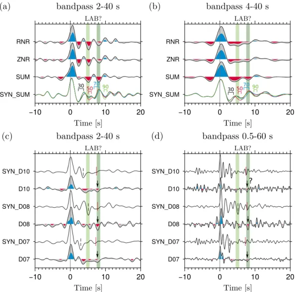
Figure 7.Comparison between synthetic ZR RFs using the models obtained byHannemann et al.[2016] (black lines in Figure 4b) and OBS data. The colored areas show where the 95% confidence level is above zero (blue) and below zero (red) for the single stations, the stack of all stations (SUM), beam-formed traces prenormalized to rms amplitude of noise on Z (ZNR) and beam-formed traces prenormalized to rms amplitude of noise on R (RNR). The faint green areas indicate the arrivals of phases probably related to the LAB. (a, b) Comparison between synthetics (SYN_SUM) and SUM, ZNR and RNR. The line colors of the synthetic RFs indicate the depths of the LAB in the used models (black: 30 km, red: 50 km, blue: 70 km, green: 90 km). The markers indicate the identified arrival of the LAB phase in the synthetics. The RFs have been band-pass filtered (2–40 s (Figure 7a) and 4–40 s (Figure 7b)). (c, d) Comparison of ZR RFs of single stations (D07, D08, and D10) with corresponding synthetics (SYN_D07, SYN_D08, and SYN_D10) for models with an LAB at 70 km depth. Black arrows indicate probable LAB phases. Black dashed markers indicate arrival ofPpPsMoho multiple and red markers of LAB phases on the synthetic traces. The delay times have been calculated based on the corresponding velocity-depth model for each station. The RFs have been bandpass filtered (0.5–60 s (Figure 7c) and 2–40 s (Figure 7d)). All RFs have been normalized to thePspike on the Z component.
Nevertheless, the single stations D07, D08, and D10—as was already pointed out—are less influenced by strong sedimentary and crustal reverberations, which is also visible in thePwave spectra (Figures B1f, B1g and B1i in the Appendix). From thePwave polarization analysis [Hannemann et al., 2016], we know that the sediments are rather thin (300–400 m) at these stations. Most of the sediment and crustal multiples therefore arrive before∼4 s (Figure 4b) and do not interfere with the later arriving negative phase at∼8 s. Furthermore, the comparison between the synthetics and the OBS RFs in Figure 4 (band pass 0.5–60 s) showed that they agree quite well in the first seconds at stations D07, D08, and D10. In Figure 7c, we observe that the shapes of synthetics for an LAB at 70 km and the real data are comparable in the first seconds for the filter band between 2 s and 40 s. The synthetics also show that thePpSsmultiple of the Moho is a much stronger negative phase
Figure 8.Band-pass filtered ZR receiver functions (7 s to 60 s).
The colored areas indicate where the 95% confidence level is above zero (blue) and below zero (red) for the RF stacks (all stations: SUM;
beam-formed traces prenormalized to the rms amplitude of noise on Z: ZNR; beam-formed traces prenormalized to the rms amplitude of noise on R: RNR). The markers indicate the position of the signals corresponding to the 410, the 660, and the probable signals of the Lehmann discontinuity (220) with 2 standard deviations estimated by picking 300 bootstrapped RFs. The RFs have been normalized to thePspike on the Z component. Solid lines show the delay times corresponding to depths of 220 km, 410 km, 520 km, and 660 km assuming PREM [Dziewonski and Anderson, 1981]. The number in front of each trace indicates the number of events which contributed to the RF stack.
at∼3–5 s, in comparison to the later arriving LAB phase (∼7–7.5 s). Further- more, the LAB phase is hard to identify in this filter band due to the interference with other multiples. For shorter periods (band pass 0.5–60 s, Figure 7d), we can identify small negative phases at∼8 s at D07, D08, and D10, although the phase at D10 remains questionable due to sim- ilar earlier negative phases. Neverthe- less, we have to be aware that at these short periods we are approaching the limits of resolution of our data; there- fore, we have to be careful with inter- preting the observations. The observed phases at∼8 s (marked by black arrows in Figures 7c and 7d) arrive a bit later than the LAB phases in the correspond- ing synthetic RFs and indicate a prob- able sharp LAB. Their delay times cor- respond to LAB depths between 70 km and 80 km if the sediment and crustal structure obtained byPwave polariza- tion is assumed at the single stations.
For a lithospheric age between 75 Ma and 85 Ma as in this study (Figure 9) [afterMüller et al., 2008], the observa- tion of an LAB in 70–80 km depth would be in line with depth observations made for similar ages in the Pacific [Rychert et al., 2012, Figure 6].
In summary, we conclude that there might be a probable sharp LAB at∼70–80 km, for which we find weak evidence at single stations with rather thin sediments (300–400 m). Furthermore, we notice that strong sed- imentary and crustal reverberations mask the arrival of the LAB phase and need to be considered in the discussion or modeling of potential LAB phases.
4.3. Upper Mantle Discontinuities
ThePsconverted phases caused by the 410 and 660 should arrive∼44 s and∼68 s after the directPphase and have positive amplitudes. These amplitudes are several tens of times smaller than the directPphase (compare
́ ṔP410
́
ṔS410 and ṔṔ́́PS660
660 in Figure 2c). The usual approach to enhance them is stacking. In Figure 8, we present the band-pass filtered (7–60 s) stacked ZR RFs of the single stations (SUM) and beam-formed traces with different prenormalizations (ZNR and RNR). The delay times shown as guidance correspond to depths of 220 km, 410 km, 520 km, and 660 km assuming PREM [Dziewonski and Anderson, 1981]. For the upper mantle, we can clearly identify one positive phase at∼68–69 s (Table 2) and a second low-confidence phase at∼43–46 s (Table 2). We associate the phase at∼43–46 s with the 410 and the phase at∼68–69 s with the 660.
The expected delay time for the 410 assuming PREM velocities is 43.97 s, which agrees quite well with the measured delay times of the stacks of the single stations (43.11±1.26 s) and is similar to the measured delay times of the beam-formed traces (ZNR: 46.46±2.13 s, RNR: 45.76±1.31 s). This indicates a normal depth of the 410, which is in good agreement with observations made bySaki et al.[2015] in their precursor study.
The expected delay time for the 660 assuming PREM is 68.26 s. The measured delay times are similar (SUM:
68.01±0.41 s, ZNR: 69.46±1.18 s, and RNR: 69.26±0.78 s). AlthoughSaki et al.[2015] provide only a few depth estimates for the 660, our observations match theirPPprecursor estimates north and south of our OBS array.
Transforming delay times of the mantle discontinuities to pseudodepths is usually strongly influenced by the velocity model of the uppermost mantle and crust. It is therefore common practice to employ more robust
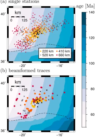
Figure 9.Location of piercing points of upper mantle discontinuities for (a) single stations and (b) beam-formed traces (estimated for the center of the array). The age of the oceanic lithosphere in million years [Müller et al., 2008] is shown by the color shading. The piercing points are shown for depths of 220 km (yellow circles, Lehmann discontinuity), 410 km (orange circles), 520 km (black crosses), and 660 km (red circles). The locations of the OBSs used are indicated as black triangles. The position of the Eurasian-African plate boundary (Gloria Fault) [Bird, 2003] is marked as a black dashed line.
estimates like the delay time difference between the 660 and the 410 [e.g.,Gu and Dziewonski, 2002]. This difference is 24.9±1.33 s (Table 2) for the single station stack (SUM), 23.00±2.44 s (Table 2) for the stack of the beam-formed traces normalized to the noise on the Z component (ZNR), and 23.50±1.52 s (Table 2) for the stack of the beam-formed traces normalized to the noise on the R component (RNR). This difference between the 410 and the 660 is similar to the theoretical estimate using PREM (24.29 s) within the error bounds.
A small time shift of the MTZPsphases can be observed (∼1.5 s, Table 2) between the single stations’ stack and the stack of the beam-formed traces. We investigate whether this observed time shift of the 410 and 660 is related to the different processing of the single stations and the beam-formed traces by calculating synthetic RFs using a full wave field reflectivity method (QSEIS) [Wang, 1999] with our station distribution, a global veloc- ity model (PREM) [Dziewonski and Anderson, 1981] and a local crustal model (CRUST1.0) [Laske et al., 2013].
We find no difference in the estimated delay times of the mantle discontinuities for the beam-formed traces stack and the stack of the single stations. The small time shift in the delay times between the single stations stack and the beam-formed traces stack (Figure 8) may therefore indicate a difference in the velocities or the thicknesses of the lithosphere and mantle above the 410 sampled by the according rays.
Examining the map showing the piercing points (Figure 9), we find that the RFs mostly sample structures within the Eurasian plate (north of the Gloria Fault) for back azimuths between∼200∘and 80∘. The azimuthal coverage is similar for the single stations and the beam-formed traces. It is therefore likely that the small time shift between the different stacks is caused by the method-specific differences in the weighting according to the noise (i.e., the prenormalization to the rms amplitude of the noise).
Table 2.Delay Times for Stacked Traces and Beam-Formed Traces for Lehmann (220), “410,” and “660” Discontinuitiesa
Station t220(?)(s) t410(s) t660(s)
SUM 21.96±0.35 (43.11±1.26) 68.01±0.41
ZNR (22.84±1.92) (46.46±2.13) 69.46±1.18
RNR 22.46±0.82 (45.76±1.31) 69.26±0.78
PREM 23.81 43.97 68.26
aThe times are estimated by picking the corresponding phase on 300 stacked traces which were formed by bootstrapping the contributing traces. The times are given with an error of 1 standard deviation. Estimates in brackets represent low confidence delay time picks as indicated in Figure 8.
There is another low-confidence signal at a delay time of∼22–23 s (Figure 4 and Table 2). This signal arrives slightly earlier than would be expected for a depth of 220 km in PREM (23.81 s, Figure 8). The association of this phase with the Lehmann discontinuity is difficult, as it has a low confidence level and likely interferes with crustal and lithospheric multiples (see first 20 s in Figures 6a, 6b, and 8).
In addition, a low-confidence, weak signal is visible at∼56 s on the T components of the beam-formed traces, the arrival of which is delayed compared to the expected arrival of the “520” from PREM (54.92 s, see Figure 8).
Onsets on the T component of RFs can be caused by dipping layers or shear wave splitting in anisotropic layers [e.g.,Cassidy, 1992;Savage, 1998;Farra and Vinnik, 2000]. The oceanic upper mantle is anisotropic in global models like PREM and shows lateral and depth-dependent variations of anisotropy in surface wave-based tomography models [Pilidou et al., 2005]. However, it is hard to identify signals on the R component (Figure 8) which might represent a split shear wave component near the T component signal at∼56 s. If this signal originates due to anisotropy in a layer above 520 km depth, shear waves converted at 660 km depth should be split as well. This is not observable in Figure 8. The limited number of available RFs, as well as their often low signal quality hinder the formation of back azimuth-dependent stacks with a sufficient confidence level.
The latter would be required to constrain a possible anisotropy component in the data. The cause of this signal therefore remains enigmatic.
In summary, the usage of beamforming techniques increases the number of events available for the RF analy- sis and therefore also the SNR of the RF. In combination with bootstrapping and uncertainty estimations, they help to estimate the confidence of signals originating from deeper mantle structures as the MTZ.
5. Conclusion
This study shows that it is possible to identify discontinuities in the oceanic crust and upper mantle down to the MTZ using OBS data. Furthermore, it explores the advantages of using beamforming to improve the signal quality of RFs and a quality control employing evaluation criteria such as relative spike position and SNR to search for the optimal deconvolution length. In this study, we demonstrate that these techniques work well.
The first analyzed discontinuity is the Moho, for which the average pseudodepth is∼5 km estimated using PREM velocities. This is slightly less than would be expected for oceanic crust in general [e.g.,White et al., 1992;
Laske et al., 2013]. The RFs show evidence for the presence of a sediment layer at the single stations which likely influences the estimated delay times and therefore the pseudodepths. Furthermore, possible crustal multiples indicate a Moho depth of∼7–8 km which is more in line with the expected values [e.g.,White et al., 1992;Laske et al., 2013].
Second, we focus on the asthenosphere. The interpretation of the LAB and the Lehmann discontinuity is dif- ficult because of simultaneously arriving reverberations of sediment, crustal, and lithospheric structures and requires synthetic modeling to understand the observed effects. The synthetic modeling indicates that the influence of sedimentary and crustal reverberations masks the arrival of the LAB phase for the stack of all sta- tions and the normalized beams. Nevertheless, at single stations with thin (300–400 m) sediments, a weak negative phase indicates a probable sharp LAB at∼70–80 km depth. These estimates are in line with depth estimates for similar ages in the Pacific [Rychert et al., 2012]. A positive phase arrival at∼22–23 s on the RF stacks may correspond to the Lehmann discontinuity [e.g.,Deuss et al., 2013] but likely interferes with crustal and lithospheric multiples.
We find that the 410 and the 660 are located at depths expected from PREM and are in line with a recent precursor study in this area [Saki et al., 2015]. A delay between the 410 and the 660 signal observed at the single stations stack and the beam-formed traces stack is likely caused by the different prenormalization of the data before the RF calculation.
In conclusion, this study shows that the number of usable events for RF studies at the ocean bottom can be more than doubled in comparison to single station approaches using beamforming techniques at a midaper- ture array. This approach is especially promising if deeper mantle features with small amplitudes are to be investigated as it increases the SNR of the event recordings and the number of usable events for the analysis of OBS RFs. The application of evaluation criteria supports the selection of optimal deconvolution time window lengths. Nevertheless, a manual revision of the RFs resulting from the preselected deconvolution lengths is still necessary to exclude RFs from the analysis that are influenced by high-frequency noise. Furthermore, this study proves that the combination of single OBSs and beamforming techniques gives the opportunity to investigate structures from the sea floor down to the MTZ. The analysis of the localSwave velocity structure viaPwave polarization [Hannemann et al., 2016] proves to be useful in understanding the effects encountered by sedimentary and crustal reverberations at single OBSs using synthetic modeling.
Appendix A: Orientation
We test two different approaches to estimate the orientation of the OBSs (i.e., angle between geographic north and the north component of the seismometer): (1) using thePwave polarization on the horizontal components, and (2) using the phase shift of the Rayleigh wave between the vertical and radial components.
For the analysis of thePwave polarization, we measure the amplitudes of several teleseismicPphases on all three components for each station. We estimate the theoretical amplitude distribution of thePphase on the horizontal components by using the verticalPwave polarization and the known back azimuth of the earthquake. After a stepwise rotation of the theoretical amplitude distribution, we calculate the difference (misfit) between the theoretical and the measured horizontal amplitudes.
We estimate this misfit for several events and calculate the mean and standard deviation. We use the defi- nitions of mean,𝜇, and standard deviation,𝜎, from directional statistics analogous toGrigoli et al.[2012] for Nmeasurements of the orientation angle,𝜑i, with weightwi, which is chosen based on event quality.
𝜇=arctan(Q P )
∧ 𝜎=√
2⋅(1−R) with P=
∑N i=1
wicos𝜑i ∧ Q=
∑N i=1
wisin𝜑i
andR= 1
∑N i=1wi
√P2+Q2
(A1)
Furthermore, we combine the misfit functions of all events by calculating the mean of the different misfit functions for each tested angle.
Table A1.Results of Orientation of OBSs (i.e., Angle Between Geographic North and the North Component of the Seismometer) Using thePPhasea
Station No. of Events Single Events All Events Bootstrap
D01 9 144.8∘ ±27.6∘ 144∘ 144.2∘ ±5.3∘
D02 8 195.5∘ ±17.5∘ 198∘ 198.5∘ ±3.5∘
D03 13 177.2∘ ±34.2∘ 175∘ 175.5∘ ±2.3∘
D04 7 94.1∘ ±28.9∘ 98∘ 99.5∘ ±7.3∘
D06 15 56.1∘ ±49.0∘ 57∘ 57.8∘ ±5.2∘
D07 14 203.3∘ ±32.8∘ 202∘ 202.1∘ ±2.8∘
D08 7 239.4∘ ±31.1∘ 228∘ 233.9∘ ±10.6∘
D09 12 142.4∘ ±32.8∘ 139∘ 141.7∘ ±7.1∘ D10 11 271.1∘ ±51.3∘ 261∘ 262.6∘ ±5.4∘ D11 11 349.6∘ ±34.2∘ 351∘ 351.4∘ ±2.9∘ D12 11 289.7∘ ±53.9∘ 300∘ 298.3∘ ±7.1∘
aWe present the results of the analysis of single events, the combined misfit function and the bootstrap. The mean and standard deviation are calculated using equation (A1).
Table A2.Results of Orientation of OBSs (i.e., Angle Between Geographic North and the North Component of the Seismometer) Using the Rayleigh Phasea Station No. of Events Single Events All Events Bootstrap
D01 24 140.3∘ ±13.7∘ 142∘ 140.4∘ ±2.2∘
D02 28 193.7∘ ±13.0∘ 195∘ 193.1∘ ±2.3∘
D03 28 164.9∘ ±12.9∘ 166∘ 164.5∘ ±2.2∘
D04 27 99.1∘ ±17.4∘ 98∘ 96.8∘ ±2.2∘
D06 25 48.5∘ ±25.7∘ 49∘ 48.0∘ ±2.5∘
D07 20 197.9∘ ±8.9∘ 197∘ 196.9∘ ±1.8∘
D08 18 226.2∘ ±11.1∘ 228∘ 225.8∘ ±2.6∘
D09 21 138.6∘ ±8.0∘ 137∘ 136.6∘ ±2.2∘
D10 11 252.2∘ ±13.9∘ 254∘ 251.2∘ ±3.0∘
D11 18 349.2∘ ±10.5∘ 349∘ 348.5∘ ±2.9∘
D12 21 299.7∘ ±15.5∘ 300∘ 300.2∘ ±3.1∘
aWe present the results of the analysis of single events, the correlation coef- ficient of the concatenated data, and the bootstrap. The mean and standard deviation are calculated using equation (A1).
We also use surface waves to estimate the orientation of the stations [Stachnik et al., 2012]. The data are filtered with a band pass between 20 and 60 s and the horizontal components are rotated using the back azimuth of the events. If the horizontal components are properly oriented, the vertical trace will be identical to the Hilbert transform of the radial trace within the time window of the Rayleigh phase [Stachnik et al., 2012]. We decide to include the Love phase in our analysis, because its energy should completely vanish from the radial component if the components have the correct orientation. We use a normalized zero-lag cross correlation, Srz, between the Hilbert transform of the radial trace (R) and the vertical trace (Z) (equation (A2) [Stachnik et al.,̃ 2012;Zha et al., 2013].
Srz= 𝜌(R̃,Z)
𝜌(Z,Z) with 𝜌(X,Y) =
∫
t2 t1
X(t)Y(t)dt (A2)
Figure A1.Estimated orientation of OBSs byPphase polarization (red arrows and slices) and Rayleigh wave ellipticity (black arrows and open slices). The arrows show the estimated directions of the north component of the seismometer and the slices the error of the orientation (see also Tables A1 and A2).
Figure B1.Mean spectra for all events used at the single stations (D01–D12) and for the unnormalized beam traces (PLN) (Tables C1 and C2) in the Appendix. Spectra for vertical (Z, black), radial (R, blue), and transversal (T, red) recordings ofPwaves were calculated for 200 s long seismograms starting 50 s before thePwave arrival. Additionally, the lighter colors show the mean spectra of the preevent noise which were calculated for a 200 s long time window starting 250 s before thePwave arrival.
Herein,𝜌(R̃,Z)
is the zero-lag cross correlation between the Hilbert transform of the radial trace and the ver- tical trace and𝜌(Z,Z)is the zero-lag autocorrelation of the vertical trace. Before calculatingSrz, we normalize the traces. The horizontal traces are equally treated to preserve the particle polarization. Afterward, we rotate the horizontal traces in 1∘steps and calculateSrz. As for thePphase, we estimateSrzfor several events
and calculate the mean and standard deviation according to equation (A1). Furthermore, we append all event data and process them together.
Moreover, we use the bootstrap method and equation (A1) to estimate mean and standard deviation for the combined misfit function for thePphase and the correlation coefficient for the Rayleigh phase. The resulting angles are presented in Table A1 for thePphase and in Table A2 for the Rayleigh phase and in Figure A1.
Appendix B: Additional Figures
Figure B1 shows the mean spectra for all single stations and for the unnormalized beams using 200 s long seismograms ofPwaves (dark colors) and pre-event noise (light colors). Figure B2 shows slowness bin stacks
Figure B2.(bottom) Stacks of single stations RFs in slowness bins of 0.5 s/∘every 0.25 s/∘. Light green area shows expected delay times for an interface at 40–50 km depths and dark green area for an interface at 65–75 km assuming PREM [Dziewonski and Anderson, 1981]. The small number at the end of each slowness bin stack indicates the number of events in the bin. (top) Move-out corrected stacks for stack of all stations (SUM) and single stations D07, D08, and D10 as already presented in Figure 6a. The RFs have been band-pass filtered (2–40 s) and normalized to thePspike on the Z component.