Effects of High CO2

(1)

Master’s Thesis

Effects of High CO

2

on Immune Response and Scale Structures in Juvenile Turbot

(Scophthalmus maximus)

By

Huajing Yan

Thesis Advisors

Prof. Thorsten Reusch (Evolutionary Ecology of Marine Fishes, GEOMAR)

Prof. Stanislav Gorb (Functional Morphology and Biomechanics, Zoological Institute, CAU) Joanna Miest (Evolutionary Ecology of Marine Fishes, GEOMAR)

Marlene Spinner (Functional Morphology and Biomechanics, Zoological Institute, CAU) Catriona Clemmesen-Bockelmann (Evolutionary Ecology of Marine Fishes, GEOMAR)

May 2016

(2)

(3)

ABSTRACT

Ocean acidification (OA), a consequence of the dissolution of excess anthropogenic carbon dioxide in ocean water, is ongoing worldwide. Possible effects of ocean acidification on marine organisms include impacts on growth and development, survival, reproduction, acid-base regulation, behavior, and biomineralizing species calcification rates. The health and well-being of organisms depends on their immune system, therefore one part of this thesis was to study the effect of ocean acidification on the immunity. Another part is in regards to the effect of ocean acidification on biomineralization; in this thesis is fish with biomineralizing scales, which could also influence the health of an organism. Early life stages are highly vulnerable; therefore this thesis studied juvenile turbot (Scophthalmus maximus) response to the effects of elevated carbon dioxide (CO2) levels on the innate immune system and scale structures.

Turbots were exposed to three different levels of CO2 (ambient, 1000 µatm and 2000 µatm) in both short term (1 week) and long term (16 weeks) exposure. In the short term experiment, a stress response in the highest CO2 treatment was observed, evident from an increase in lysozyme activity which led to a downregulation of an antimicrobial peptide (hepcidin1). No CO2 effect was found in the long term experiment on both the immune response and scale structure, suggesting the ability of turbots to acclimate to future predicted oceanic CO2 levels. However changes in gene expression and lysozyme activity in the long term experiment suggested a stress effect from seasonal temperature variations.

(6)

2

(7)

3

1. INTRODUCTION

Industrialization and human population growth has resulted in increased use of fossil fuels, deforestation, and cement production which has caused a great increase of carbon dioxide CO2, the primary greenhouse gas, in the atmosphere (Caldeira & Wickett, 2003). Atmospheric gas and dissolved oceanic gas are in equilibrium, therefore, oceans act as a major sink for atmospheric CO2 and the increase in CO2 in the atmosphere has led to an increase in the ocean CO2 (Levine & Doney, 2006). The Intergovernmental Panel on Climate Change (IPCC) predicts that the global mean oceanic CO2 values are expected to reach 1,000 ppm CO2 by year 2100, causing a pH decrease of 0.3-0.4 (IPCC, 2014), and could reach 1,900 ppm CO2 by year 2300 (Caldeira & Wickett, 2003; IPCC, 2007). However, many coastal regions around the world are already seeing levels of CO2

that match global predictions beyond year 2100 (Melzner et al., 2013).

The carbonate system in the ocean consists of dissolved CO2, HCO3-, and CO32-

which are at chemical equilibrium (Dickson et al., 2007). An increase in CO2 therefore leads to an increase in HCO3- and decreases in CO32-, with also an increase in H⁺ (hydrogen ions), resulting in the disturbance of the entire carbonate system with a decrease in pH causing ocean acidification.

Ocean acidification has many consequences on marine organisms. Calcifying organisms are particularly affected (Riebesell et al., 2000). Many studies on species with calcium carbonate skeletons such as calcifying phytoplankton, molluscs, crustaceans, and echinoderms have shown that acidification has caused reduced rates of calcification and significant shell dissolution in these organisms (Riebesell et al., 2000; Feely et al., 2004). The formation of biogenic calcium carbonate (CaCO3) which is a key building component for many organisms that form shells or plates (Hernroth et al., 2012) is decreased or even prevented under low ocean pH. For the formation of calcium carbonate, calcium ions (Ca²⁺) and carbonate ions (CO32-) which are both present in seawater are combined together by these organisms. When ocean acidification occurs, an increase of CO2 reacting with H2O causes an increase of hydrogen ions (H⁺) which bind to carbonate ions with greater attraction than calcium ions (Fabry et al., 2008).

When this occurs, shell-forming organisms can no longer use the carbonate ions to form new shells or skeletons and if there are more hydrogen ions than free carbonate ions,

(8)

4

this could even lead to shell dissolution when the hydrogen ions start breaking down carbonate from existing shells and skeletons (Guinotte & Fabry, 2008).

However, not only shelled organisms are impacted by ocean acidification.

Studies on fish have shown physiological changes due to increased CO2 such as changes in growth, organ development, reproduction, larval development, or behavior (Frommel et al., 2011; Frommel et al., 2014; Heuer & Grosell, 2014; Ishimatsu et al., 2004; Munday et al., 2014). Compensatory internal acid-base regulation is hypothesized to be responsible for these physiological and behavioral alterations (Heuer & Grosell, 2014).

To ensure homeostasis and acid-base stability, regulation of ion transporting proteins such as NHE or V-type H⁺-ATPase can be modified to compensate for the change of internal pH levels (Souza et al., 2014; Gilmour & Perry, 2009).

Since internal regulation is costly, other physical functions have to be compromised in order to survive in a high CO2 environment; therefore it is believed that fish’s immune system could also be affected by this regulation for survival. It has been seen in studies on invertebrates such as the green sea urchin (Strongylocentrotus droebachiensis), a sea star (Leptasterias polaris), the blue mussel (Mytilus edulis), and the Norway lobster (Nephrops norvegicus) that their immune responses have been impacted due to ocean acidification (Bibby et al., 2008; Dupont & Thorndyke 2012;

Hernroth et al., 2012). However, no knowledge is yet available on the impact of high CO2

on vertebrate immune system response.

The fish immune system is physiologically similar to higher vertebrates and consists of the innate and adaptive immune system (Uribe et al., 2011). The innate immune system consists of proteins and cells that are always present but nonspecific and the adaptive immune system, which is specific, is activated when the pathogen passes the innate immune system. The difference between fish and higher vertebrates is that in fish the nonspecific immunity is the fundamental defense mechanism due to limitations of the adaptive immune system (Uribe et al., 2011). Various factors can influence the innate immune response such as temperature, light, water quality, salinity, stress, or food additives (Uribe et al., 2011).

(9)

5 The fish used in this experiment, turbot (Scophthalmus maximus) is a highly prized flatfish and one of the most commercially important fish in aquaculture (Zhang et al., 2011). It is distributed along the coast of Europe in the Northeast Atlantic, Mediterranean Sea, Baltic Sea, up until the Norwegian Sea (Exadactylos et al., 2007).

Turbot are abundant in coastal waters with shallow soft bottom habitats and feed on crustaceans and fish (Froese & Pauly, 2015) and have been known to grow up to 100 cm long and weigh 25 kg (Exadactylos et al., 2007).

Turbot, and other flatfish, have modified elasmoid scales called tubercles on their skin (Faílde et al., 2014). These tubercles are small, isolated, mineralized conical plates randomly distributed in the pigmented side of the body which originate from thin and flat plates located in the skin of larvae and juveniles, whose structure is that of regular- developing elasmoid scales (Zylberberg et al., 2003; Murcia et al., 2015). Since these tubercles undergo biomineralization like the shells of shelled organisms, and are partly exposed to the water, ocean acidification could also affect the growth process and material properties of these modified scales and influence the health of the fish.

Apart from studies showing that elevated CO2 can alter calcification rates or carbonate dissolution, it could also impact the structure of the calcifying skeleton itself.

Studies by Gutowska (2010) showed that cuttlebone from cephalopod Sepia officinalis, which consists of aragonite (CaCO3) and undergoes biomineralization, experienced changes in mineralized structures under elevated CO2. Since turbot scales also consists of mineralizing materials, ocean acidification could also impact the fundamental structure of the tubercle scale itself, therefore altering the mechanical properties of the scale.

In this study, a short term experiment of 1 week and a long term of 16 weeks were performed. Heuer & Grosell (2014) mentioned in their paper that “abrupt and relatively short-term CO2 exposures are inherently limiting in their ability to assess the adaptive capacity of a species” and a study by Stiller et al., (2015) found that turbot in their studies could acclimatize to hypercapnic conditions after two weeks. Therefore an experiment investigating an acute and chronic exposure can provide knowledge into the response of turbot immune responses to ocean acidification and possible acclimation.

(10)

6

Early life stages of fish are found to be less tolerant than adult life stages to environmental toxicity (Hutchinson et al., 1998) and high juvenile mortality have been observed in marine invertebrates (Gosselin & Qian, 1997), therefore juvenile turbots were used in this study. We studied the effect of two levels of elevated CO2, ~1000 µatm from end of century predictions and ~2000 µatm from year 2300 predictions, on the innate immune system and tubercle scale properties of juvenile turbot. The innate immune system parameters that were measured were lysozyme activity, blood cell composition, and immune gene expression. Adaptive immune genes were also analyzed for a full immune response picture along with other non-immunity genes to provide a better understanding of any effects found from innate immune gene response. The scale properties were measured by nanoindentation on turbot tubercles.

Nanoindentation methods used in this experiment followed methods developed by Oliver and Pharr (1992;2004), which measured hardness and elastic modulus of a material by indentation at nanometer scales. Oliver and Pharr’s method can determine mechanical properties of small-sized materials such as thin films and small structural features, which could be obtained directly from indentation load-displacement measurements.

The hypotheses to be tested within this study are that:

1. Increased CO2 has an effect on the immune system gene expression in dependence of treatment time.

2. Increased CO2 effects biomineralization of the fish scale, resulting in altered mechanical properties.

(11)

7

2. MATERIALS & METHODS

2.1 ANIMALS

The experiment was conducted in two parts, a short term experiment of 1 week, and a long term experiment lasting 16 weeks.

Juvenile turbot (Scophthalmus maximus) were acquired from Stolt Sea Farm in Norway in 2014. They were reared in GEOMAR’s NEMO Hall with flow through Baltic Sea water at ambient conditions prior to the experiment. At the beginning of the short term experiment, the turbots weighed 170.8 ± 5.2 g and measured 20.4 ± 0.2 cm in length (head-tail length). In the long term study, the turbots weighed 126.1 ± 3.3 g and had a length of 18.5 ± 0.2 cm at the start experiment.

In the short term experiment, all fish were fed with turbot feed from Skretting (R-3 Europa 22%) every morning at 0.2% of fish body weight. Fish from the long term experiment were fed with the same type of food every morning, however the amount was adjusted every week to 0.5% of the average fish weight per each tank. In both experiments, fish were kept on a restrictive diet following values from Sæther and Jobling (1999). All food was eaten and all the tanks were cleaned daily.

In order to allow individual analysis of the fish in the long term experiment each animal received a colour tag on their dorsal fin.

(12)

8

2.2 EXPERIMENTAL SET UP

The experiment consisted of a short term 1 week experiment and a long term 16 week experiment. Both experiments consisted of 3 treatments: ambient CO2 (i.e control), medium CO2 (approx. 1000 µatm), and high CO2 (approx. 2000 µatm). All treatments were run with 4 replicate tanks each and each tank contained 3 turbots totaling 12 tanks and 36 turbots for each experiment (Fig. 1).

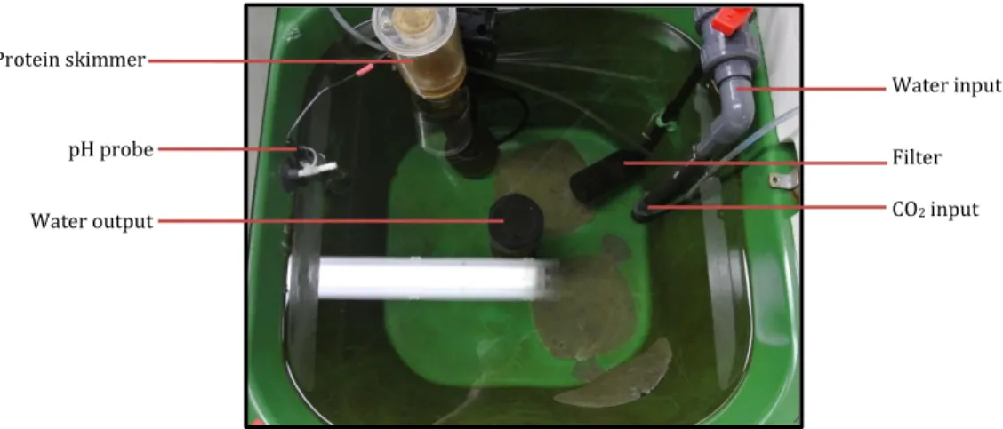
The experimental tanks were 60 L in volume, with continuous flow through Baltic water from the Kiel Fjord at a flow rate of 400 ml/min. These tanks rested in a large holding tank filled with Baltic Sea water. Additionally each tank was fitted with a filter and a protein skimmer while the CO2 treated tanks also contained a CO2 tube and pH probe connected to a computer system (Fig. 2).

Figure 1: Experimental set up of both studies

Figure 2: Equipment in each tank

Water input

Filter CO2 input Water output

pH probe Protein skimmer

(13)

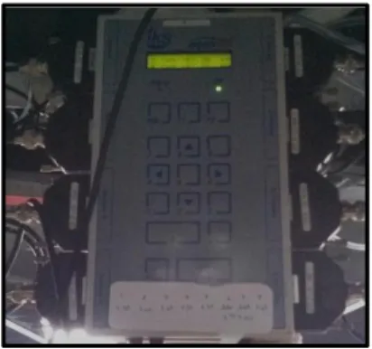
9 The iks aquastar computer system (iks ComputerSysteme GmbH, Germany) was used to monitor the pH levels in each tank (Fig. 3). Each CO2-treated tank had a pH probe and CO2 tube connected to the iks system. The target pH value for each tank was programmed into the system controlling the CO2 valve in order to maintain the targeted pH value.

The water temperature in the experimental tanks varied with the water temperature of the Fjord but was kept at 20°C maximum through the hall’s air condition system and the large water body of the holding tanks. Light intensity was set to approximately 30 lux with an interval of 11:13 light: dark. The pH, salinity, and temperature of each tank were monitored daily. The pH was measured with a pH Electrode (SenTix 81, Wissenschaftlich-Technische Werkstätten GmbH, Germany) calibrated with NBS buffer while salinity and temperature were measured with a conductivity probe (TetraCon 325 and Multi 350i, Wissenschaftlich-Technische Werkstätten GmbH, Germany). Water quality was checked periodically by measuring dissolved oxygen with an oxygen probe (CellOx 325, Wissenschaftlich-Technische Werkstätten GmbH, Germany), measuring ammonium with Tetra Test NH3/NH4+ kit (Spectrum Brands, Inc. USA), and measuring nitrite with Tetra Test NO2- kit (Spectrum Brands, Inc. USA).

Figure 3: iks aquastar computer system used for pH monitoring

(14)

10

2.3 WATER ANALYSIS

Water samples were taken weekly by filling and overflowing the bottles with a plastic tube from the tank into the bottom of the sample bottle. This avoids air bubbles and washes out the bottles. All samples were immediately poisoned with a saturated HgCl2 solution (0.5 ‰ final concentration) for storage. Samples for total alkalinity (TA) measurements were stored in plastic bottles and dissolved inorganic carbon (DIC) samples were stored in airtight glass bottles at room temperature.

Total alkalinity of the water samples was analyzed with Metrohm 862 Conpact Titrosampler and the results were calculated with MATLAB script supplied by Kai Schulz, GEOMAR, Kiel, Germany (2005) and DIC was measured using an AIRICA system (Marianda) via a LI-COR 7000 infrared CO2/H2O analyser. Both TA and DIC values were then corrected using the Dickson seawater standard as reference material. The pCO2

was calculated from measured DIC and pH values using CO2SYS software (Pierrot et al.

2006) with dissociation constants from Mehrbach et al. (1973) as refitted by Dickson and Millero (1987) and KHSO4 dissociation constant after Dickson (1990).

2.4 SAMPLING

In the long term exposure, all fish were weighed, measured and 100 µl of blood was taken from the caudal vein with a 0.4 x 19 mm (Nr. 20) needle and 1 ml syringe (Becton, Dickson and Company, USA) every two weeks. 20 µl of the blood sample was suspended in 1 ml of RPMI Medium 1640 (Gibco, Thermo Fisher Scientific Inc. USA) for flow cytometry analysis and the rest of the blood was stored in Heparin microtubes (Sarstedt AG & Co, Germany) for lysozyme activity analysis. To measure growth, specific growth rate was calculated with^{(ln 𝑊𝑒𝑖𝑔ℎ𝑡}^{𝐹𝑖𝑛𝑎𝑙}^{−ln 𝑊𝑒𝑖𝑔ℎ𝑡}^{𝐼𝑛𝑖𝑡𝑖𝑎𝑙}^{) 𝑥 100}

𝑑𝑎𝑦𝑠 . Final condition

factors were calculated from the equation of Arfsten et al. (2010) for flatfish

𝑤𝑒𝑖𝑔ℎ𝑡 𝑥 100

(𝑙𝑒𝑛𝑔𝑡ℎ 𝑥 𝑤𝑖𝑑𝑡ℎ)³^⁄² and Fulton’s condition factor 𝑤𝑒𝑖𝑔ℎ𝑡 𝑥 100 𝑙𝑒𝑛𝑔𝑡ℎ³ .

At the end of both short and long term experiments, all turbots were anaesthetized and blood and organ samples (gills, spleen, gut, liver, kidney, head kidney, and skin) were collected. Blood samples were used in flow cytometry and lysozyme activity analysis, and organ samples were stored in RNA stabilization reagent

(15)

11 (RNAlater) at -80 °C for molecular genetic analysis. Hepatosomatic index (HSI) of the long term study fish was calculated with (liver weight/fish weight) x 100 and spleen- somatic index (SSI) was calculated with (spleen weight/fish weight) x 100.

The tubercles of fish from the long term experiment were removed from the skin along the lateral line, rinsed with clean water, left to air dry over night, and stored for nanoindentation analysis.

2.5 FLOW CYTOMETRY

Live cells in turbot blood were analyzed with flow cytometry, a method where cells are identified and counted by size and morphology using their specific light characteristics. Fresh blood samples suspended in RPMI media (Gibco, Thermo Fisher Scientific Inc. USA)were washed twice with 1 ml RPMI by centrifuging with 6000 g for 10 min at 4 ˚C and discarding the supernatant. The samples were re-suspended in 450 µl RPMI and used for cell count analysis.

For the analysis, 150 µl of the samples were mixed with 100 µl of 20 µg/ml propidium iodide (Carl Roth GmbH, Germany) and 150 µl RPMI, and analyzed with a BD Accuri C6 Flow Cytometer set for a limit of 10,000 events in ‘cells’. The amount of monocytes and lymphocytes measured in percentage were then calculated into proportions relative to all live cells measured from the sample, following Landis et al., 2012.

2.6 LYSOZYME ACTIVITY

The rest of the blood sample was centrifuged with 1400 g for 5 min at room temperature, the serum or supernatant was collected in microcentrifuge tubes and stored at -20˚C for lysozyme activity analysis using the Sigma-Aldrich Lysozyme Activity Kit according to the manufacturer’s protocol. 0.01% (w/v) stock Micrococcus bacteria solution was prepared before each week’s measurements by dissolving Micrococcus lysodeikticus in the reaction buffer until the absorbance (450 nm) was 0.6-0.7 compared to a buffer blank. 25 µl of serum from each sample was mixed with 175 µl stock bacteria solution and immediately measured in a Tecan Infinite M200 spectrophotometer at 450 nm absorbance for a duration of 30 min in 30 sec intervals.

(16)

12

After measurements, the lysozyme concentration was calculated by the following equation: Units/ml enzyme = ^(∆𝐴⁴⁵⁰𝑇𝑒𝑠𝑡/ min − ∆𝐴₄₅₀𝐵𝑙𝑎𝑛𝑘/min )(𝑑𝑓)

(0.001)(𝑣𝑜𝑙𝑢𝑚𝑒 𝑚𝑙) Where df = dilution factor, 0.001 = ΔA450 as per the Unit Definition (one unit lysozyme produces ΔA450 of 0.001 per minute at pH 6.24 and 25˚C using Micrococcus lysodeikticus suspension as substrate in 2.6 ml reaction mixture), and volume = 0.1 (enzyme solution volume in ml).

2.7 MOLECULAR GENETIC ANALYSIS

2.7.1 RNA Extraction & cDNA Synthesis

Gills, spleen, head kidney, and skin samples from both long term and short term experiments were thawed over ice. Approximately 20 mg of these organ samples were used for RNA extraction with Stratec InviTrap Spin Universal RNA Kit. RNA extraction was conducted according to the manufacturer’s protocol. Samples were placed in 900 µl Lysis Solution TR adjusted with 1/100 volume of β-Mercaptoethanol and homogenized with Zirconia beads from the kit (4 beads á 0.7mm & 2 beads á 1.2mm) using a TissueLyser II (QIAGEN GmbH, Germany) for 5 min at 25 Hz. The samples were then centrifuged and the supernatant was transferred into a new tube and mixed with 500 µl of molecular grade ethanol. The solution was pipetted onto the spin column and further washing steps followed the manufacturer’s instruction with 30 µl of Elution Buffer R used at the end for elution. RNA concentration was measured with Nanodrop ND-1000 (Peqlab, Germany) and all samples were diluted to 100 ng/µl with RNase-Free water.

RNA samples were stored at -80°C.

Genomic DNA in RNA samples was removed using Quanta PerfeCta DNase I Kit (Quanta BioSciences, Inc. USA). For each sample, 8.5 µl (i.e. 850 ng) of RNA template were mixed with 1 µl 10x Reaction Buffer and 0.5 µl PerfeCta DNase I for a total reaction volume of 10 µl. The reaction mix was incubated using a thermocycler (PTC-200 Peltier Thermal Cycler, Bio-Rad Laboratories, Inc. USA) for 30 min at 37˚C, 1 µl of 10x Stop Buffer was then added into each mix and incubated for 10 min at 65˚C. The final product was then used for cDNA synthesis.

(17)

13 cDNA was synthesized using Quanta qScript cDNA Synthesis Kit (Quanta BioSciences, Inc. USA). For each sample, 7.5 µl of RNA was mixed with 2 µl of qScript Reaction Mix (5x) and 0.5 µl of qScript RT for a final volume of 10 µl. The reaction mix was then run in the thermocycler (PTC-200 Peltier Thermal Cycler, Bio-Rad Laboratories, Inc. USA) for 5 min at 22˚C, 30 min at 42˚C, and 5 min at 85˚C. The final cDNA product was stored at -20 ˚C until further use.

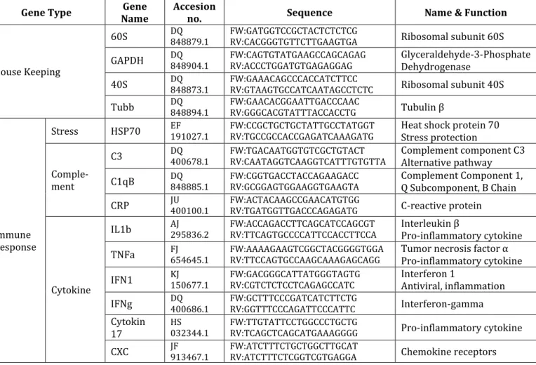
2.7.2 Primers

A total of 32 target genes were analyzed for gene expression including genes for housekeeping, stress, apoptosis, glycolysis, immune response, antioxidant, and osmoregulation. 30 primers were designed by Joanna Miest (Miest & Bray, in prep;

Miest et al., 2016) and 2 primers for osmoregulation, Carbonic Anhydrase and V-type H⁺- ATPase, were designed with BLAST search (NCBI) and Primer 3 Plus specifically for real-time PCR with a melting temperature of 60˚C. Table 1 belows lists the complete list of primers used in this experiment.

Table 1: List of primers used in this experiment

Gene Type Gene

Name Accesion

no. Sequence Name & Function

House Keeping

60S ^DQ_848879.1 FW:GATGGTCCGCTACTCTCTCG

RV:CACGGGTGTTCTTGAAGTGA Ribosomal subunit 60S GAPDH ^DQ_848904.1 FW:CAGTGTATGAAGCCAGCAGAG

RV:ACCCTGGATGTGAGAGGAG Glyceraldehyde-3-Phosphate Dehydrogenase

40S ^DQ_848873.1 FW:GAAACAGCCCACCATCTTCC

RV:GTAAGTGCCATCAATAGCCTCTC Ribosomal subunit 40S Tubb ^DQ_848894.1 FW:GAACACGGAATTGACCCAAC

RV:GGGCACGTATTTACCACCTG Tubulin β

Immune Response

Stress HSP70 ^EF_191027.1 FW:CCGCTGCTGCTATTGCCTATGGT

RV:TGCCGCCACCGAGATCAAAGATG Heat shock protein 70 Stress protection

Comple- ment

C3 ^DQ_400678.1 FW:TGACAATGGTGTCGCTGTACT

RV:CAATAGGTCAAGGTCATTTGTGTTA Complement component C3 Alternative pathway C1qB ^DQ_848885.1 FW:CGGTGACCTACCAGAAGACC

RV:GCGGAGTGGAAGGTGAAGTA Complement Component 1, Q Subcomponent, B Chain CRP ^JU_400100.1 FW:ACTACAAGCCGAACATGTGG

RV:TGATGGTTGACCCAGAGATG C-reactive protein

Cytokine

IL1b ^AJ_295836.2 FW:ACCAGACCTTCAGCATCCAGCGT

RV:TTCAGTGCCCCATTCCACCTTCCA Interleukin β

Pro-inflammatory cytokine TNFa ^FJ_654645.1 FW:AAAAGAAGTCGGCTACGGGGTGGA

RV:TTCCAGTGCCAAGCAAAGAGCAGG Tumor necrosis factor α Pro-inflammatory cytokine IFN1 ^KJ_150677.1 FW:GACGGGCATTATGGGTAGTG

RV:CGTCTCTCCTCAGAGCCATC Interferon 1

Antiviral, inflammation IFNg ^DQ_400686.1 FW:GCTTTCCCGATCATCTTCTG

RV:GGTTTCCCAGATTCCCATTC Interferon-gamma Cytokin

17 ^HS^032344.1 FW:TTGTATTCCTGGCCCTGCTG

RV:TCAGCTCAGCATGAAAGGGG Pro-inflammatory cytokine CXC ^JF_913467.1 FW:ATCTTTCTGCTGGCTTGCAT

RV:ATCTTTCTCGGTCGTGAGGA Chemokine receptors

(18)

14

Mucosal Mucin18 ^JU 370277.1

FW:TTGTCCCTGACCAAGTGATG

RV:ACAAAGCCTGTCCAAGATCG Mucus forming Mucin2 ^JU_403288.1 FW:TGTTGGAGCAAGGAGAAACC

RV:TTGTCTCAGGTTGGCAGTTG Mucus forming Adaptive

Immune Response

CD45 ^FJ_226005.1 FW:GCGACTTCTGGTTGATGGTT

RV:TGTCTGTGCTTGCAACTTCC Cluster of differentiation 45 CD8 ^JU_368863.1 FW:TTACATGGCTTCTGCTGCTG

RV:AATGGCTGAAGTGCTTTGCT Cluster of differentiation 8 MHCII ^HQ_698612.1 FW:AACAAGCTGGAGGTCACGAG

RV:TTTCCCACGTTGATGAGACA Major histocompatibility complex class II

Innate Immune Response

Anti- microbial peptide

Hep1 ^AY_994075.1 FW:CTCCCTTTGCCGCTGGTG

RV:AGCCCTTGTTGGCCTTGC Hepcidin 1 Hep2 ^JQ_219840.1 FW:ATGAAGACTCTCACCGTTGC

RV:TTCTGTCTGTTACTCGGCATC Hepcidin 2 gLys ^HQ_148717.1 FW:TCTCATTGCTGCCATCATCTC

RV:CCACTCGGATTAACATCAACCT g-type Lysozyme Bactericidal cLys ^AB_355630.1 FW:GAACGCTGTGAATTGGCCCGACT

RV:GTTGGTGGCTCTGGTGTTGTAGCTC c-type Lysozyme Bactericidal beta-

defensin1 ^JU^362659.1 FW:GGGAAAGGCTTCTTGTGTTG

RV:TCTGTCCTATCTCCTGTGATGC Antimicrobial beta-

defensin3 ^JU352527.1

FW:GGAATGGCAAATGCTCAGAC

RV:CATCGCTCAATGGTTTCTCC Antimicrobial TLR3 ^FJ_009111.1 FW:GACGTGCTGATCCTGGTCTTTCTGG

RV:AGCTCAGGTAGGTCCGCTTGTTCA Toll like receptor 3

Pattern recognition receptor Trans ^AJ_277079.1 FW:TTTGGCTTCCAGGATCTCCAG

RV:CAGCTTTCGAGGAAGAAGTTGC Transferrin Anti-bactericidal

Osmoregulation CA ^JU_378925.1 FW:ACTCCAATGGCATCCTCAAC

RV:TGTTCCAGAAATGGGACCTC Carbonic anhydrase Ion exchange HATPase ^JU_389146.1 FW:TCACAGACGGAAAGTGCTTC

RV:TTCAGCCACACTTGGTATCG V-type H⁺-ATPase Ion exchange Antioxidant SOD ^HS_029499.1 FW:AAACAATCTGCCAAACCTCTG

RV:CAGGAGAACAGTAAAGCATGG Superoxide dismutase Antioxidant defense Tight Junction Cadherin ^HS_032161.1 FW:ATGGGACACGCTATGACACA

RV:ATCTCCATTTGCGTCGTGAT Tight junction

Apoptosis Caspase3 ^JU

391554.1

FW:TTCTGCCATTGTCTCTGTGC

RV:GCCCTGCAACATAAAGCAAC Pro-apoptotic Caspase7 ^JU_373310.1 FW:TCTGCAATGTCCTCAACGAG

RV:TTGCGACCATGTAGTTGACC Pro-apoptotic Glycolysis G6P ^KC_184131.1 FW:GGAAGCAAGAAATCCAGCAG

RV:CGGCAACAATCATACCTGTG Glucose-6-phosphate p450 ^JN_216889.1 FW:AGACGAGCAATGGAAGAGGA

RV:GAAAGCAGTGCTGGTCACAA Cytochrome p450 Metabolism

2.7.3 Gene Expression Analysis using qPCR (Gills)

Since only osmoregulation genes (2 genes) were analyzed in turbot gill samples, gene expression was measured with real-time quantitative PCR. The gill cDNA was diluted with water (PCR grade) at a 1:10 dilution before the analysis. The reaction mix composed of 2 µl 5x HOT FIREPol EvaGreen qPCR Mix Plus (Solis BioDyne, Estonia), 0.25 µl forward primer, 0.25 µl reverse primer, 5.5 µl PCR grade H2O, and 2 µl of cDNA template. The qPCR was performed with the StepOnePlus Real-Time PCR System (Applied Biosystems/Thermo Fisher Scientific) with an incubation step at 95˚C for 15

(19)

15 min, followed by 40 cycles of 95˚C for 15 sec and 60˚C for 1 min, and ending with a meltcurve: 95˚C for 15 sec 60˚C for 1 min, and an increase of 0.5˚C/min until 95˚C.

The gene expression (ΔCt) of each sample was calculated from the geometric mean of the housekeeping genes and used in statistical analysis. For illustration, gene expression relative to control was calculated according to the 2^-ΔΔCt method (Livak &

Schmittgen, 2001) where ΔΔCt of samples was calculated in relation to the mean ΔCt of the control group.

2.7.4 Gene Expression Analysis using the Fluidigm Biomark system (Head Kidney, Spleen, Skin)

Gene expression of all 32 genes in spleen, head kidney, and skin, was analyzed with qPCR Biomark HD system (Fluidigm, USA) based on 96.96 dynamic arrays (Gene Expression chips). Before the chip analysis, a pre-amplification step was performed.

Each pre-amplification reaction mix contained 2.5 µl TaqMan PreAmp Master Mix (Applied Biosystems), 0.5 µl STA Primer Mix (500 nM primer pool from all primers in low EDTA TE buffer), 0.75 µl H2O, and 1.3 µl cDNA. Amplification was run for 10 min at 95˚C, then 14 cycles of 15 sec at 95 ˚C and 4 min at 60 ˚C. The final product was diluted 1:10 with low EDTA TE buffer. For the chip run, each sample mix contained 3.5 µl 2x SSoFast EvaGreen Supermix with low Rox (BioRad), 0.35 µl 20x DNA Binding Dye Sample Loading Reagent (Fluidigm), and 3.2 µl pre-amplified diluted cDNA. Each primer mix contained 3.5 µl 2x Assay Loading Reagent (Fluidigm), 3.15 µl low EDTA TE Buffer, and 0.7 µl Primer PreMix (50 µM of each primer pair). The chip run then followed the Fluidigm 96/96 Gene Expression Protocol with 5 standards and a blank water sample.

The raw data was evaluated using Fluidigm Real-Time PCR Analysis software and extracted for further analysis. Primer efficiency of all primers was verified to be similar. The stability of housekeeping genes was calculated with qBase+ software and the 3 most stable genes were used as reference genes by using the geometric mean for further calculations. Gene expression (ΔCt) of each sample was then calculated in relation to the reference genes and used for statistical analysis. Gene expression relative to control was calculated for illustration according to the 2^-ΔΔCt method (Livak &

Schmittgen, 2001).

(20)

16

2.8 TURBOT SCALE MECHANICAL PROPERTY ANALYSIS

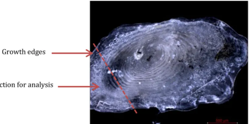
Only fish from control and highest CO2 treatment in the long term experiment were used for analysis. Single tubercles were removed from along the upper lateral line of previously frozen defrosted fish and left to dry overnight. The point of interest in this experiment was the growth region which was along the edge of the tubercle. The edge of the dried tubercles was then cut off and fixed on a sample holder with liquid plastic welder (Bondic, Laser Bonding Tech, Inc., Aurora, Canada) (Fig. 4).

To measure the mechanical properties, nano-sized indents were made on the edge of the tubercles using Nano Indenter SA2 (MTS Nano Instruments, Oak Ridge, TN, USA). The measurements were conducted at room temperature (22-25˚C) with relative humidity 40-45%. The Continuous Stiffness Measurement (CSM) method was used to measure the changes in mechanical properties (Enders et al., 2004) with a maximun penetration depth of 500 nm at a constant strain of 0.05 s^-1.

The hardness and Young’s modulus data for each sample, which provides information for the hardness and elasticity, respectively, were determined by processing load-displacement curves following methods by Oliver and Pharr (1992;2004). Data acquired from the machine was transferred into excel for graph plotting where both hardness and Young’s modulus values at each depth were averaged for every 10 nm. The value at the plateau section of the graph was used as the final value of hardness and Young’s modulus of each sample.

Figure 4: Example of a tubercle and the removed section (lower left corner)

Section for analysis Growth edges

(21)

17

2.9 STATISTICAL ANALYSIS

All statistical analysis was performed with statistical software JMP 11.2 (SAS Institute Inc. 2013). All data was checked for normality and homogeneity of variances using Shapiro-Wilk test and Levene’s test, respectively. Non normal data were transformed using log base 2. MANOVA was performed on gene expression data divided into functional gene groups. A two-way nested ANOVA was performed to analyze the effect of tank, time, treatment, and time-treatment interaction. A one-way ANOVA was performed to further investigate the effect between treatments within each time point.

If there was a significance, a post hoc Tukey HSD test was used to determine the exact difference. For data that was not normally distributed after transformation, a Kruskal- Wallis test was performed instead of a normal one-way ANOVA.

(22)

18

3. RESULTS

3.1 WATER PROPERTIES

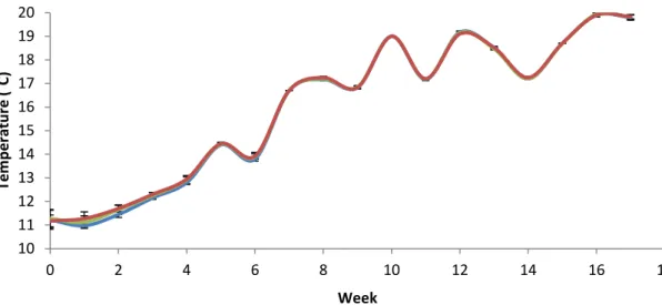
Water temperature increased throughout the course of the experiment from 10.8˚C (lowest measurement) to 19.9˚C (highest measurement) but was not different between treatments (Fig. 5). Except for pH, which was modified to mimic two different levels of ocean acidification, all other factors were kept constant throughout the experiment.

Figure 5: Mean daily water temperature (± SEM) of all treatments (calculated from 4 replicates for each treatment) throughout the experiment (blue line = ambient conditions, green line = medium pCO2 ~1000 µatm, red line = high pCO2 ~2000 µatm)

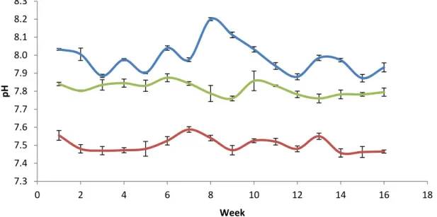
The pH in the control tanks fluctuated with the pH of the Kiel Fjord between 7.88-8.20. The pH in the medium CO2 treatment varied from 7.76–7.87 and in the high CO2 treatment from 7.45- 7.59 with no overlap between treatments (Fig. 6).

10 11 12 13 14 15 16 17 18 19 20

0 2 4 6 8 10 12 14 16 18

Temperature (˚C)

Week

(23)

19 Figure 6: Average daily pH (± SEM) of all treatments throughout experiment (blue line = ambient conditions, green line = medium pCO2 ~1000 µatm, red line = high pCO2 ~2000 µatm)

pCO2 was calculated from measured DIC and pH using CO2SYS (Lewis and Wallace, 1998) and the values for 1 week and 16 week experiment are displayed in Table 2 and 3 respectively.

Table 2: Carbonate chemistry values (± SEM) of 1 week experiment measured at start of experiment from all replicates tanks

Treatment pH (NBS)

Alkalinity (µmol/kgSW)

DIC (µmol/kgSW)

pCO2 (µatm) Control 8.10 2080.38 ± 3.93 2014.90 541.56 Medium CO2 7.77 2079.37 ± 3.15 2115.75 1218.90

High CO2 7.55 2082.22 ± 3.96 2124.52 2006.83

Table 3: Carbonate chemistry values (± SEM) of 16 week experiment measured at start of experiment and every 4 weeks after from all replicates tanks

Treatment pH

(NBS) Alkalinity

(µmol/kgSW) DIC

(µmol/kgSW) pCO2 (µatm) Control 7.98 ± 0.02 2008.23 ± 13.10 1994.97 ± 8.48 722.33 ± 38.67 Medium CO2 7.80 ± 0.01 2009.88 ± 13.77 2045.33 ± 6.16 1209.42 ± 37.38

High CO2 7.50 ± 0.01 2011.31 ± 13.30 2117.86 ± 6.78 2325.09 ± 64.22

7.3 7.4 7.5 7.6 7.7 7.8 7.9 8.0 8.1 8.2 8.3

0 2 4 6 8 10 12 14 16 18

pH

Week

(24)

20

3.2 GROWTH & CONDITION

1 Week

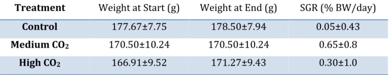
Turbot in the 1 week experiment had an average starting weight of 170.8±5.2 g and end weight of 176.9±5.3 g. Average weight and specific growth rate of each treatment can be found in table 4 below.

Table 4: Average turbot weight ± SEM and average specific growth rate ± SEM in short term experiment

Treatment Weight at Start (g) Weight at End (g) SGR (% BW/day) Control 177.67±7.75 178.50±7.94 0.05±0.43 Medium CO2 170.50±10.24 170.50±10.24 0.65±0.8

High CO2 166.91±9.52 171.27±9.43 0.30±1.0

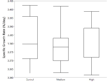
There was no significant difference between the specific growth rates between treatments in the 1 week experiment (df = 2, F = 0.2374, p = 0.7901) as seen from the boxplots in Fig. 7.

Figure 7: Specific growth rate (% Body Weight/day) between treatments of turbot from 1 week experiment. Box plot shows median, upper and lower quartile, minimum and maximum.

(25)

21 16 Weeks

The fish in the 16 week experiments had an average weight of 126±3.3 g at the start of the experiment. No significant effect on final weight was detected between treatments (Control: 199±8.54 g, medium: 208.17±6.54 g, high: 199.33±5.09 g). On average the turbot grew with a specific growth rate of 0.42±0.02 % body weight gain/day and no significant difference was detected (Fig. 8).

Figure 8: Specific growth rate (% BW/day) calculated from start to end between treatments of turbot from 16 week experiment. Box plot shows median, upper and lower quartile, minimum and maximum.

The bi-weekly specific growth rate did not differ between treatments in all time points (Fig. 9).

Figure 9: Specific growth rate (%/day) measured every 2 weeks of turbot from 16 week experiment (blue line = ambient conditions, green line = medium pCO2 ~1000 µatm, red line = high pCO2 ~2000 µatm)

-2.5 -2 -1.5 -1 -0.5 0 0.5 1 1.5 2 2.5

0 2 4 6 8 10 12 14 16

Specific Growth Rate (%/day)

Week

(26)

22

Similarly to the specific growth rates, no difference was seen in the calculated condition factors (table 5).

Table 5: Condition factors of turbots between treatments in 16 week experiment. HSI = hepatosomatic index (calculated from liver weight to body weight ratio), SSI = spleen-somatic index, (calculated from spleen weight to body weight ratio), K = condition factor (calculated from body weight and length)

Treatment HSI SSI K* K**

Mean SEM Mean SEM Mean SEM Mean SEM

Control 0.90 0.03 0.04 0.004 2.44 0.04 1.78 0.04 Medium CO2 0.90 0.04 0.05 0.003 2.44 0.03 1.75 0.02 High CO2 0.90 0.04 0.05 0.005 2.46 0.03 1.75 0.03

K* = The condition factor (CF) calculated using the weight and length data following the equation of Arfsten et al. (2010) for flatfish, CF = (weight×100)/(length×width)ˆ3/2

K** = Fulton’s condition factor = weightx100/length^3 (Froese, 2006)

3.3 LYSOZYME ACTIVITY

1 week

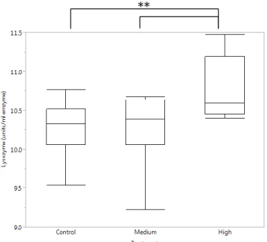
After 1 week of CO2 exposure (Fig. 10) lysozyme activity significantly increased (df = 2, F = 5.9590, p = 0.0062) in the highest CO2 treatments (1790.76±153.39 units/ml enzyme) compared to the medium CO2 (1298.78±89.75 units/ml enzyme, p = 0.0180) and the control treatment (1264.94±85.71 units/ml enzyme, p = 0.0113).

Figure 10: Lysozyme activity in turbot serum with confidence intervals in 1 week experiment (**p≤0.01). Box plot shows median, upper and lower quartile, minimum and maximum.

**

(27)

23 16 Week

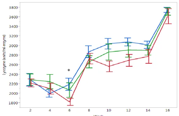
In the long term experiment, most of the lysozyme activity did not differ across treatments. However when the p values of each time point are considered, a trend is indicated that the difference between treatments becomes greater over the weeks, especially lysozyme activity in week 6 (Control: 2151±123, medium: 1940±224, high:

1825±73 units/ml enzyme, p = 0.0498), until week 10 (lysozyme activity Control:

3043±111, medium: 2869±169, high: 2568±112, p = 0.0518) and then the difference gradually disappears until the end of the experiment (Fig. 11).

Figure 11: Mean lysozyme activity ± SEM in turbot serum measured every 2 weeks in 16 week experiment (blue line = ambient conditions, green line = medium pCO2 ~1000 µatm, red line = high pCO2 ~2000 µatm) (*p<0.05)

*

(28)

24

3.4 GENE EXPRESSION

Treatment Effect Gills

Carbonic anhydrase (ca) expression in the gills was not significantly affected by the CO2 exposure in both the short term (df = 2, F = 0.6274, p = 0.5444) and long term experiment (df = 2, F = 0.0092, p = 0.9908) as seen from Fig. 12.

Figure 12: Mean ca gene expression (relative to control) ± SEM in turbot gills compared between treatments from 1 week and 16 week experiments

V-type H⁺-ATPase average gene expression was not affected by the CO2 exposure at any time point. However time significantly affected gene expression in the medium CO2 treatment (t = 3.61, df = 22, p = 0.0016) (Fig. 13). In the short term study, V-type H⁺- ATPase gene expression of 1.02±0.07-fold (Δct = 6.99±0.09) was higher in this treatment than in the long term study of 0.69±0.06-fold (Δct = 7.61±0.15). Though statistically not significant (p=0.16), the Control group also displayed a trend of H⁺- ATPase down regulation in the long term experiment (1 week: 1.13±0.15-fold, Δct = 7.13±0.24, 16 week: 0.80±0.06-fold, Δct = 7.51±0.11). Statistical tests showed that v- type H⁺-ATPase gene expression in gills was not significantly influenced by the CO2

treatments in both the 1 week (df = 2, F = 0.6730, p = 0.5177) and the 16 week experiment (df = 2, F = 1.5584, p = 0.2260).

16 Week 1 Week

Control Medium High Control Medium High

(29)

25 Figure 13: V-type H⁺-ATPase gene expression (relative to 1 week study) ± SEM in turbot gills compared between time from 1 week and 16 week experiments (**p≤0.01)

Head Kidney

Multivariate analysis of head kidney gene expression in short term study revealed that genes involved in immunity (c3, il1b, tnfa, c1qb, cd8, cytokin 17, cxc, mhcii, cd45, glys, clys, tlr3, beta-defensin1&3, crp, ifn1, ifng, mucin2&18, hsp70), osmoregulation (ca & H⁺-ATPase), antioxidant (sod), tight junction (cadherin), and glycolysis (g6p &

p450) were not affected by elevated CO2 levels. Antimicrobial genes however were significantly affected by CO2 treatments (F=2.54, p=0.0304) as well as apoptosis genes (F=2.88, p=0.0301).

Upon further investigation into apoptosis genes, caspase 3 was found to be significantly down regulated (df = 2, F = 6.6012, p = 0.0063) in the highest CO2

treatment (0.80±0.05-fold, Δct = 5.13±0.08) compared to Control (1.02±0.06-fold, Δct = 4.79±0.09) in the short term experiment (Tukey HSD p = 0.0169) (Fig. 14).

Similarly at the same time point, gene expression of hepcidin-1, from antimicrobial gene group, in the high CO2 treatment (0.59±0.08-fold, Δct = 7.07±0.19) was significantly down-regulated (df = 2, F = 5.1625, p = 0.0116) compared to Control (1.16±0.21-fold, Δct = 6.20±0.23, p = 0.0144) and medium CO2 treatment (0.93±0.14- fold, Δct = 6.65±0.40, p = 0.0428) (Fig. 14).

**

Control Medium High

(30)

26

Figure 14: Caspase-3 and Hepcidin-1 (Hep1) gene expression (relative to control) ± SEM from turbot head kidney between treatments from 1 week experiment (*p<0.05, **p≤0.01)

Following a similar pattern found in the short term experiment, MANOVA revealed an effect of CO2 on apoptosis genes (F=2.52, p=0.0495) in the long term study, which was expressed in the decrease of caspase 7 expression (df = 2, F = 6.4551, p = 0.0397) of the high CO2 treatment (0.71±0.04-fold, Δct = 6.47±0.08) compared to the Control group (1.08±0.14-fold, Δct = 5.95±0.17, Tukey HSD p = 0.0455) (Fig. 15).

Also in the long term study, mucus genes were found to be effected by treatment (F=4.03, p=0.0060). Further analysis revealed a down regulation of mucin 2 (df = 2, F = 3.9149, p = 0.0317) in the medium CO2 treatment (0.36±0.09-fold, Δct = 17.14±0.41) compared to the high CO2 treatment (3.85±1.61-fold, Δct = 14.33±0.66, Tukey HSD p = 0.0455) (Fig. 15).

** *

(31)

27 Figure 15: Mucin-2 and Caspase-7 gene expression (relative to control) ± SEM from turbot head kidney between treatments from 16 week experiment (*p<0.05)

Spleen

Multivariate analysis on spleen gene expression revealed that most genes were not affected by an increase in CO2 in the short term study, such as immunity genes, (c3, il1b, tnfa, c1qb, cd8, cytokin 17, cxc, mhcii, cd45, hep2, glys, clys, tlr3, beta-defensin1&3, crp, ifn1, ifng, trans, mucin2&18, hsp70), osmoregulation genes (ca & H⁺-ATPase), antioxidant gene (sod), tight junction gene (cadherin), glycolysis genes (g6p & p450), and apoptosis genes (caspase3&7).

As already seen in head kidney hepcidin 1, in the short term study, spleen hepcidin 1 in high CO2 (0.63±0.10-fold, Δct = 7.15±0.22) was also down regulated (df = 2, F = 3.5126, p = 0.0414) compared to the Control (0.95±0.13-fold, Δct = 6.50±0.19;

Tukey HSD p =0.0347) (Fig. 16).

Another gene affected by CO2 was sod, which was up regulated (df = 2, F = 9.0319, p = 0.0109) in the short term study, with the medium CO2 treatment gene expression (1.27±0.08-fold, Δct = 2.68±0.09) higher than both the Control (1.01±0.05- fold, Δct = 2.99±0.07, p = 0.0226) and the high CO2 treatment (0.87±0.07-fold, Δct = 3.26±0.14, p = 0.0062) (Fig. 16).

Interestingly, these effects disappeared during long term CO2 exposure, when no differences in gene expression were detected in spleen.

* *

(32)

28

Figure 16: Hepcidin-1 (Hep 1) and sod gene expression (relative to control) ± SEM from turbot spleen between treatments from 1 week experiment (*p<0.05)

Skin

Gene expression in skin tissue was only analyzed for the ambient and high treatment. Only cadherin was found to be affected by elevated CO2 levels. During the 1 week experiment, cadherin was up regulated (t = -3.27, df = 16, p = 0.0048) in the high CO2 treatment (2.64±0.27-fold, Δct = 6.82±0.16) compared to Control treatment (1.27±0.25-fold, Δct = 8.15±0.41) (Fig. 17). No differences in gene expression were observed at 16 weeks.

Figure 17: Cadherin gene expression (relative to control) ± SEM from turbot skin between treatments from 1 week experiment (**p≤0.01)

**

Control High

* *

(33)

29 Time Effect

Although treatment did not affect mRNA levels of most genes, some of the studied genes were influenced by the duration of the treatment (Fig. 18). In turbot head kidney some genes (c3, ca, caspase 3, gapdh, glys, sod) were up-regulated in the long term exposure compared to the acute exposure independent of treatment (df =1, F > 9, p < 0.003) (Fig. 18A). As for the spleen, both up- and down-regulated genes were found in the long term treatment (df=1, F>11, p<0.0014) which can be seen in Fig. 18B and 18C. All gene expressions were relative to the Control group of the 1 week experiment.

Figure 18: Mean gene expression relative to short term Control ± SEM from 1 week and 16 week experiments in turbot head kidney (A) and spleen (B&C)

B) Spleen C) Spleen

A) Head Kidney

Control Medium High Control Medium High Control Medium High Control Medium High Control Medium High Control Medium High

(34)

30

3.5 BLOOD COUNT

1 Week

The analysis of blood cell composition of fresh turbot blood from week 0 and week 1 of the short term experiment showed that at the start of the study (week 0), fish had a lymphocyte proportion on average (relative to all live cells) of 0.52±0.03 and a monocyte average proportion of 0.56±0.02. No significant effect of final lymphocyte (Control: 0.57±0.03, medium: 0.60±0.02, high: 0.65±0.01) and monocyte proportion (Control: 0.54±0.03, medium: 0.50±0.02, high: 0.46±0.01) was detected between treatments or time (Fig. 19).

Figure 19: Mean proportion of lymphocytes (A) and monocytes (B) relative to all live cells

±SEM in fresh turbot blood from 1 week experiment

16 Week

As for the long term study (Fig. 20), monocytes (df=2, F=4.5844, p=0.0175) and lymphocytes (df=2, F=4.6742, p=0.0163) at almost all time points were not affected by CO2, except for week 16. In the last week of the long term study, average proportion of lymphocytes in the medium treatment (0.74±0.02) was significantly higher (Tukey HSD p=0.0215) than the Control (0.66±0.02). Monocytes displayed an opposite trend, with average proportion monocytes in medium CO2 treatment (0.37±0.02) significantly lower (Tukey HSD p=0.0260) than the Control (0.45±0.02).

A) Lymphocytes B) Monocytes

Control Medium High Control Medium High Control Medium High Control Medium High

(35)

31 Figure 20: Bi-weekly mean proportion of lymphocytes (A) and monocytes (B) relative to all live cells ± SEM in fresh turbot blood from 16 week experiment (blue line = ambient conditions, green line = medium pCO2 ~1000 µatm, red line = high pCO2 ~2000 µatm) (*p<0.05)

A) Lymphocytes

B) Monocytes

*

(36)

32

3.6 SCALE MECHANICAL PROPERTIES

Images of turbot scales, also referred to as tubercles, were obtained with a stereo light microscope Leica M205A (Leica, Wetzlar, Germany) at 20 X and 50 X magnification (Fig. 21). Images reveal that most of the tubercle, including the growth region of interest, lies under the skin (Fig. 21A & 21B). Shape and size of the whole tubercle can be seen after removal from the skin in Fig. 21C & 21D.

Figure 21: Stereo light microscopy images of turbot tubercle at 20X and 50X magnification captured before removal (A&B) and after removal from skin (C&D)

Turbot scale properties were only analyzed in the ambient and high CO2

conditions of the long term experiment. Measurements from 200nm-500nm into the surface contained the most constant values; therefore the average measurement values from this region were used for comparison of elastic modulus and hardness between treatments.

A) 20 X B) 50 X

C) 20 X D) 50 X

(37)

33 Young’s Modulus

In the 16 week experiment, tubercle analysis determined the average Young’s modulus, or elastic modulus, between 200-500 nm depth of the Control group to be 5.31±0.13 GPa and the high CO2 group to be 4.78±0.10 GPa (Fig. 22). A lower Young’s modulus value represents a more flexible material, and similarly a high modulus value signifies a more stiff material. Statistical analysis revealed no significant effect of CO2 on the Young’s modulus of the turbot tubercle (t = -1.66, df = 18, p = 0.1144).

Figure 22: Average Young’s Modulus of turbot tubercle from Control (A) and high CO2 (B) treatment. Blue line represents average modulus, dotted lines represent the upper and lower standard error of mean (SEM)

0 1 2 3 4 5 6

0 100 200 300 400 500 600

Modulus (GPa)

Displacement into surface (nm) A) Control

0 1 2 3 4 5 6

0 100 200 300 400 500 600

Modulus (GPa)

Displacement into surface (nm) B) High CO2

(38)

34 Hardness

As for the hardness measurements, similar to the Young’s modulus results, there was no significant difference of scale hardness (t = 0.10, df = 18, p = 0.9192) between turbots from the Control group (0.163±0.011 GPa) and the high CO2 treatment (0.165±0.004 GPa) between 200-500 nm depth in the long term study (Fig. 23).

Figure 23: Average hardness of turbot tubercle from Control (A) and high CO2 (B) treatment.

Blue line represents average hardness, dotted lines represent the upper and lower standard error of mean (SEM)

0 0.02 0.04 0.06 0.08 0.1 0.12 0.14 0.16 0.18 0.2

0 100 200 300 400 500 600

Hardness (GPa)

Displacement into surface (nm)

0 0.02 0.04 0.06 0.08 0.1 0.12 0.14 0.16 0.18 0.2

0 100 200 300 400 500 600

Hardness (GPa)

Displacement into surface (nm) A) Control

B) High CO2

(39)

35

4. DISCUSSION

This study was conducted to investigate the effect of elevated CO2 on immune response and scale mechanical properties of juvenile turbots. Turbots are a commercially important fish in aquaculture (Froese & Pauly, 2015) and this study is beneficial for understanding the acclimation potential of turbots to increasing CO2

levels. Knowledge of their response to future predicted levels of oceanic CO2 is essential to predict the impacts of ocean acidification on fisheries and aquaculture production which in turn is relevant to climate change policies and management.

As suggested by Heuer & Grosell (2014) short term CO2 exposure experiments have limited ability in assessing species’ adaptive capacity, and juvenile turbots in a study by Stiller et al. (2015) were able to acclimatize to hypercapnic conditions after two weeks, the experiment in this study therefore consisted of two parts. A short term experiment to analyze acute effects on immunity and a long term experiment of 16 weeks, in order to investigate the acclimation ability of turbot’s immune responses over time, was performed.

4.1 WATER PROPERTIES

Throughout both experiments all abiotic factors were kept similar between treatments. pH levels were experimentally manipulated and led to a difference in pCO2

concentrations. Temperatures varied throughout the course of the experiment following the seasonal Kiel Fjord water temperature but were similar between treatments. Even though pH levels fluctuated, partially due to the fluctuation of pCO2 in the Baltic Sea water (Melzner et al., 2013; Thomsen et al., 2013), mean pH values of each treatment did not overlap, suggesting CO2 concentration to be the cause of treatment effects in this study. Carbonate chemistry revealed a relatively high CO2 concentration in the control groups, which was due to the high CO2 levels in seawater of the Kiel Fjord and Kiel Bay (Melzner et al., 2013) and were not removed in the experimental tanks.