Implications of land use change in tropical northern Africa under global warming

(1)

www.earth-syst-dynam.net/6/769/2015/

doi:10.5194/esd-6-769-2015

Implications of land use change in tropical northern Africa under global warming

T. Brücher^1,a, M. Claussen^1,2, and T. Raddatz¹

1Max Planck Institute for Meteorology, Hamburg, Germany

2Centrum für Erdsystemforschung und Nachhaltigkeit (CEN), Universität Hamburg, Hamburg, Germany

anow at: GEOMAR, Helmholtz Centre for Ocean Research, Kiel, Germany

Correspondence to: T. Brücher (tbruecher@geomar.de)

Received: 29 May 2015 – Published in Earth Syst. Dynam. Discuss.: 22 June 2015 Revised: 10 November 2015 – Accepted: 30 November 2015 – Published: 10 December 2015

Abstract. A major link between climate and humans in tropical northern Africa, and the Sahel in particular, is land use and associated land cover change, mainly where subsistence farming prevails. Here we assess possible feedbacks between the type of land use and harvest intensity and climate by analysing a series of idealized GCM experiments using the Max Planck Institute Earth System Model (MPI-ESM). The baseline for these experiments is a simulation forced by the RCP8.5 (radiation concentration pathway) scenario, which includes strong greenhouse gas emissions and anthropogenic land cover changes. The anthropogenic land cover changes in the RCP8.5 scenario include a mixture of pasture and agriculture. In subsequent simulations, we replace the entire area affected by anthropogenic land cover change in the region between the Sahara in the north and the Guinean Coast in the south (4 to 20^◦N) with either pasture or agriculture. In a second set-up we vary the amount of harvest in the case of agriculture. The RCP8.5 baseline simulation reveals strong changes in the area mean agriculture and monsoon rainfall. In comparison with these changes, any variation of the type of land use in the study area leads to very small, mostly insignificantly small, additional differences in mean temperature and annual precipitation change in this region. These findings are only based on the specific set-up of our experiments, which only focuses on variations in the kind of land use, and not the increase in land use, over the 21st century, nor whether land use is considered at all. Within the uncertainty of the representation of land use in current ESMs, our study suggests marginal feedback between land use changes and climate changes triggered by strong greenhouse gas emissions. Hence as a good approximation, climate can be considered as an external forcing: models investigating land-use–conflict dynamics can run offline by prescribing seasonal or mean values of climate as a boundary condition for climate.

1 Introduction

Northern Africa, and the Sahel in particular, are known to be highly vulnerable to climate change (Low, 2005; Boko et al., 2007) with regional hotspots of high national to sub- national differences in vulnerability (Busby et al., 2014).

Food production is sensitive to changes in climate across tropical northern Africa, where economies strongly depend on agriculture or livestock. When reduced precipitation and droughts affect water security and crop yield (Busby et al., 2014), human security for a growing population is at stake

(Scheffran et al., 2012). In turn, climate in this region is affected by changes in land surface conditions (e.g. Xue and Shukla, 1993; Claussen, 1997; Zeng et al., 1999; Taylor et al., 2002; Koster et al., 2004; Vamborg et al., 2011; Patricola and Cook, 2010). Therefore, it is conceivable that changes in the type and intensity of anthropogenic land use and land cover change, perhaps caused by local or national conflict, will affect regional climate.

When modelling the interaction between climate change, land use, and conflict, the question of feedbacks between climate change and changes in land use and conflict arises. If

(2)

climate change triggered any conflict and if this conflict led to major changes in land use and land cover, how strong would be the feedback of these land cover changes on climate change? If the feedback is strong, then any model that attempts to describe the nexus between climate change, land use, and conflict would have to couple climate dynamics, the dynamics of land cover change and the dynamics of conflict.

If the feedback is weak, then climate change can be considered as an external driver, or external boundary condition, of land cover and conflict dynamics.

Usually climate parameters such as growing season means or monthly means of minimum and maximum temperature are used as input for statistical or offline driven impact models like crop models (e.g. Veron et al., 2015; Scheffran and BenDor, 2009; Lobell et al., 2007, 2006). Therefore we focus here on climatological values as well, by considering annual means of temperature and precipitation.

To study possible feedback of conflict-induced land cover changes on climate without knowing the effect of climate change on conflict or the effect of conflict on land cover change, we consider a simplified set-up of numeri- cal climate simulations. We start with climate simulations of greenhouse-gas-induced global warming and consistently derived anthropogenic land cover change as defined in the RCP (radiation concentration pathway) scenarios (see be- low). In these scenarios, anthropogenic land cover change includes a mixture of agriculture and pasture. Assuming that conflict in the semi-arid regions of tropical northern Africa often arises between farmers and herders (Scheffran et al., 2012), we consider extreme scenarios by replacing the entire area allocated to land cover change in these regions either by agriculture or by pasture. Furthermore, we vary the degree of harvest generally by a constant factor without changing the type of land use. Please note that for comparison reasons in all experiments the temporal course in the fraction of land allocated to land use stays the same.

Our area of interest (in the following referred to as AOI) is located in the transition zone between the Sahara in the north and the humid Guinean Coast of west Africa in the south (4 to 20^◦N; 17^◦W to 40^◦E; in the following marked by grey boxes, e.g. as shown in Fig. 2).

2 Model and method

2.1 Model description

We use the Max Planck Institute Earth System Model (MPI- ESM; Giorgetta et al., 2013), which consists of the coupled general circulation models ECHAM6 (Stevens et al., 2013) and MPIOM (Jungclaus et al., 2013) for the atmosphere and the ocean, respectively. Marine biogeochemistry is described by HAMOCC5 (Ilyina et al., 2013), and land surface processes by JSBACH (Reick et al., 2013; Schneck et al., 2013).

JSBACH includes dynamic vegetation (Brovkin et al., 2009;

Reick et al., 2013) and land use transitions (Reick et al., 2013) according to Hurtt et al. (2011).

Within JSBACH, grid boxes over land are divided in a non-vegetated part (e.g. desert) and a vegetated one; the latter one is seperated into managed land (shrubs and pasture) and natural vegetation (woody types plus grasses). This partitioning is not given for the underlying hydrological, as this version includes a single-bucket approach. Therefore, all plant function types (PFTs) in one grid box can access the same soil water bucket at the same time, even though these tiles are physically located apart in the real world. The size of the desert area is determined by the dynamic vegetation model of JSBACH based on a function of the annual maximum filling of the green carbon pools, which are finally driven by atmospheric CO2, temperature, and precipitation.

The desert fraction increases unless the green pools are filled to maximum level at least once a year.

As the parametrization of managed land for crops and pasture are different, changes in prescribed anthropogenic land cover change (ALCC) will effect the modelled land surface in JSBACH. Generally, managed land such as pasture and crops is protected against fire, while natural grasses (and forest) are not. Pasture and crops use different photosynthetic pathways (Raddatz et al., 2007), and crops have a higher productivity, as they are parameterized by a higher carboxy- lation rate per leaf area (Kattge et al., 2009). Grazing is 2 times higher for pasture than for crops, which is parameterized by a higher herbivory and a higher leaf shedding over pasture land. Leaf regrowth is limited by NPP (net primary productivity) for grass and pasture, while it is assumed that crops have a constant leaf regrowth after sowing. The parameters for the specific carbon content per leaf are identical. Al- though visible and near-infrared albedo of the plants are the same for crops and pasture, the annual cycle in the albedo (combination of plant albedo and surface reflectivity) will be different for crops and pasture, because (i) the two differ in their phenology, (ii) the maximum leaf area index (LAI) is higher over crops, and (iii) a higher clumpiness factor for crops is simulated to mimic e.g. access roads.

2.2 Experimental set-up

2.2.1 Baseline scenario and transition rules for changes in land use and land cover

Within the framework of the Coupled Model Intercompari- son Project Phase 5 (CMIP5) three starting dates out of a con- trol simulation for pre-industrial climate by MPI-ESM have been chosen as starting points for an ensemble simulation (three members) of historic climate until 2005, called HIST.

Atmospheric CO₂concentration and ALCC were prescribed as an external forcing for MPI-ESM. For the simulation of future climate these three ensemble members are continued (at least until 2100) based on three different RCP scenarios each (RCP8.5, RCP4.5, RCP2.6). In this study, we consider

(3)

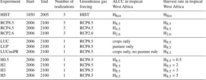
Table 1.List of experiments and their basic set-up with respect to prescribed anthropogenic land cover change (ALCC), harvest rate, and prescribed greenhouse gas forcing.

Experiment Start End Number of Greenhouse gas ALCC in tropical Harvest rate in tropical

realizations forcing West Africa West Africa

HIST 1850 2005 3 HIST H_hist H_hist

RCP8.5 2006 2100 3 RCP8.5 H_8.5 H_8.5

RCP4.5 2006 2100 3 RCP4.5 H_4.5 H_4.5

RCP2.6 2006 2100 3 RCP2.6 H_2.6 H_2.6

LUC 2006 2100 1 RCP8.5 crops only H_8.5

LUP 2006 2100 1 RCP8.5 pasture only H_8.5

LUCnoPR 2006 2100 1 RCP8.5 crops only, no pasture rule H_8.5

H0.5 2006 2100 1 RCP8.5 H_8.5 H_8.5×0.5

H2 2006 2100 1 RCP8.5 H_8.5 H_8.5×2

H3 2006 2100 1 RCP8.5 H_8.5 H_8.5×3

H5 2006 2100 1 RCP8.5 H_8.5 H_8.5×5

H_x·ymeans forcing used after Hurtt et al. (2011) according to RCP_x·y.

the simulation based on the strongest greenhouse gas forcing (RCP8.5, ca. 927 ppm CO₂ at year 2100) as a baseline scenario and put it into context with the other RCP scenarios. The RCP8.5 scenario also includes the strongest ALCC forcing (see also Fig. 4c–e).

The change of land cover is prescribed as transitions from natural to managed land or from one type of land use to an- other type of land use, which are taken from the harmonized land use protocol for CMIP5 (Hurtt et al., 2011), which pro- poses different future pathways for each RCP. By enabling land use, the so-called “pasture rule” is implemented in JS- BACH that determines which part of the natural land (grass or woody type) is taken to introduce new managed land (c.f.

Reick et al., 2013; for more details see also Appendix A1).

Annual mean harvest data are also taken from the harmonized land use protocol (Hurtt et al., 2011). These data prescribe the above-ground carbon that is taken from the above- ground biomass (for more details see also Appendix A2).

2.2.2 Set-up of sensitivity studies

All experiments (Table 1) are performed with the identical CMIP5 version of the MPI-ESM spanning the historic time period (1850–2005, HIST) or the next century (2006 to 2100). Only within AOI (4 to 20^◦N; 17^◦W to 40^◦E; see e.g.

boxes in Fig. 1) do we modify the land cover change scenarios by prescribing different anthropogenic land use and land cover change story lines.

Within the historic simulation, land use is considered in terms of crops and pasture. As we are interested in the impact of different types of land use (crops vs. pasture) on climate, we transform all managed land within the first model year (year 2006) to crops (experiment LUC, land use crops only) or pasture (experiment LUP, land use pasture only), so the to-

Fig. 4: Spatial distribution of strong anthropogenic land use transitions in pasture (left column) and crops (right column) within the ﬁrst year (2006) of the land use

experiments LUP (top row) and LUC (bottom row).

0.30 0.25 0.20 0.15 0.10 0.05 -0.05 -0.10 -0.15 -0.20 -0.25 -0.30 [m2 m^-2]

LUPLUC

Pasture Crops

30N

EQ

30S

30N

EQ

30S

0 30E 0 30E (a)

(c)

(b)

(d)

Figure 1.Spatial distribution of pasture (a) and crop (d) land use at the end of the historic simulation. The panel also shows the prescribed transitions from crops to pasture (scenario LUP; first row) and vice versa (scenario LUC, LUCnoPR; bottom row) for the first model year (2006) in the extreme land use experiments LUP, LUC, and LUCnoPR.

tal area of managed land is identical. In the following years (2007–2100) of these sensitivity studies, the transitions of natural land to managed land prescribed by the RCP8.5 scenario (Hurtt et al., 2011) to crops or pasture are summed up and natural land is only converted to crops (LUC) or pasture (LUP). Following this conversion scheme, we ensure in all experiments the same proportion of managed to natural land, which allows us to compare the results of the experiments to investigate the impact of land use. The third scenario, LUC-

(4)

Figure 2.Ensemble mean of the cover fraction([m²m⁻²) of managed land (top), natural vegetation (middle), and desert fraction (bottom) at the end of the historical simulation (year 2005) simulated by MPI-ESM. The managed land is shown for (a) pasture, (b) crops, and (c) total fraction. The natural vegetation is shown for (d) woody vegetation, (e) grass land, and (f) total separately.

noPR (land use crops only, no pasture rule), helps to separate the effect of land use and an artificial effect on the dynamical vegetation by the pasture rule (see Sect. 3.2). In experiment LUCnoPR the LUC scenario is repeated, but we bypass the pasture rule. Technically, the transitions are identical to our reference simulation RCP8.5, but we implement on all pasture areas the phenology of crops. Doing this, we ensure that the size of managed land and the partitioning of the natural land remain identical to the reference simulation RCP8.5.

To investigate the effect of low and high harvest intensity on climate, we repeat the reference simulation RCP8.5 including crops and pasture, but we change the harvest rate for crops by multiplying the RCP8.5 harvest rate by a factor of 0.5 (H0.5), 2 (H2), 3 (H3), and 5 (H5).

By interpreting the results of all these experiments, it has to be distinguished between the fractional and the absolute size of an area (e.g. the amount of grass or woody vegetation). JSBACH separates the vegetated part and the area without soil in a grid cell. In all scenarios described above, the prescribed fractional transitions are based on the vegetated area in the grid cell. The dynamical vegetation scheme has the ability to shrink or increase the vegetated area as a re- sponse to the climate; therefore the size in terms of square

metres may vary among the simulations, although the fractional partitioning within the vegetated area stays constant.

3 Results

The size of AOI covers some 10.48×10⁶km² (see boxes in e.g. Fig. 2). At the end of the historic simulation, i.e. in the year 2005, this area is fragmented into desert area (31 %;

3.25×10⁶km²), natural land (30 %; 3.15×10⁶km²), and managed land (39 %; 4.08×10⁶km²). The managed land is made up of 71 % pasture (2.90×10⁶km²) and 29 % C3 plus C4 crops (1.18×10⁶km²). Woody type vegetation domi- nates the natural land by more than 86 % (2.71×10⁶km²), while the grass fraction is low (14 %; 0.43×10⁶km²). The spatial distribution of natural and managed land for different plant functional types is shown in Fig. 2.

3.1 Baseline scenario RCP8.5 (2006–2100)

The increase of atmospheric CO₂ leads to an annual mean warming of up to 3.0 K to more than 5.5 K over Africa (Fig. 3d), which leads to annual mean temperatures in tropical northern Africa of up to 37^◦C. In general coastal area’s

(5)

Figure 3.(a, c) Ensemble mean annual precipitation sum (mm) and temperature (^◦C) for the first 30 years of RCP8.5 scenario (2006 to 2035) (left column) and (b, d) the difference (right column) with re- spect to the last 30 years of this century (2071 to 2100 minus 2006 to 2035). Only significant differences (ttest, 95 % significance level) are show. Both small changes in precipitation and non-significant changes are in white (b).

temperature increase is lower than the one further inland.

From the Guinean coast north to the desert, temperatures increase by up to 5 K.

Annual precipitation decreases near the west coast, while a surplus of 100 mm is simulated at the Guinean coast (Fig. 3a and b). Compared to the total annual precipitation of up to 2500 mm the increase is rather small. Only in few grid cells are changes in precipitation significant at a 95 % level (ttest).

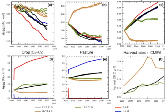
Regarding AOI, a decline in desert area (Fig. 4a) is cal- culated for all CMIP5 scenarios, which is highest for the RCP8.5 scenario (ensemble mean values: RCP2.6:−5 %/− 0.16×10⁶km²; RCP4.5:−11 %/−0.34×10⁶km²; RCP8.5:

−22 %/−0.70×10⁶km²). While higher temperatures and almost no change in precipitation put additional stress on the vegetation, these negative effects are compensated for by rising atmospheric CO2 in the MPI-ESM (Bathiany et al., 2014). Taking the ensemble mean of RCP8.5, the natural land shrinks by −27 % (−0.83×10⁶km²), as it is taken for an enlargement of land use area (37 %/1.5×10⁶km²; Fig. 4c) following the Hurtt protocol. While grazing area increases by 25 % (0.73×10⁶km²), cropland is assumed to increase by 67 % (0.81×10⁶km²) between 2006 and 2100 in the area we consider here (Fig. 4d and e). The annual amount of carbon being taken from the above-ground biomass for harvest is about 0.07 Gt C yr⁻¹in the year 2005, which is almost 10 % of the global harvest. The total area of land use enlarges by more than 37 % over the next 95 years. Harvest is assumed to double (by 0.16 Gt C yr⁻¹) due to a widening of land use

area and changes in the land use practices according to Hurtt et al. (2011).

3.2 Crop and pasture scenarios (2006–2100)

Within AOI we switch to one type of land use. In the experiment LUC all pasture is converted to crops, and in LUP all crops are changed to pasture (Fig. 1). This transition is prescribed within the first model year of the scenarios (year 2006). As land use increases within RCP8.5, the extended area is added as crops (LUC) or pasture (LUP) only, accordingly.

Within the experiment LUC the desert area shrinks further (compared to RCP8.5), while the desert area within LUP stays close to the results of our baseline scenario RCP8.5, although all simulations are forced with the same greenhouse gas scenario (Fig. 4a). These differences can be attributed to differences in the available soil water (Fig. 5). As crops are harvested, less water is used and therefore the natural vegetation will use the available soil water. This is due to the implementation of a shared water bucket for all tiles within one grid box in JSBACH. Pure pastoral land use (LUP) does not influence the available soil water, and therefore the desert area in the experiment LUP is close to the one in RCP8.5 (Fig. 4a). The area consumed for pastoral land use is almost 3 times higher than the one for crops at the end of the historical simulation (Fig. 4d and e). Therefore the scenario LUP is closer to the reference scenario RCP8.5 than LUC, because within LUP less area is converted over the first model year.

Additionally, the partitioning in natural vegetation is shifting significantly for two reasons. First, we implement a strong transition over the first model year to achieve one type of land use within LUC and LUP scenarios. Secondly, as the pasture rule is incorporated into our model, these extreme changes lead to an unbalanced partitioning in the natural vegetation that has to be compensated for by large shifts in the compounds of the natural vegetation (for more details see Appendix A1). To circumvent this artificial effect, the experiment LUCnoPR was designed, in which no artificial changes in grass or woody fraction (see Fig. 6) occur. However, the desert fraction decreases in the same manner as the LUC experiment due to the soil water differences (Fig. 4a) as managed land only consists of crops with its biophysical proper- ties and the nature to be harvested. In comparison to LUC, LUP has opposite and smaller shifts in grass and woody vegetation, but again the pasture rule is causing these effects. As grassland is used to implement pastoral land, and pasture has almost the same water usage over time as grass, the desert fraction of LUP is not significantly different to RCP8.5.

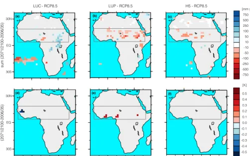
Differences in the simulated temperature and precipitation values between LUC, LUCnoPR, LUP and RCP8.5 are mostly insignificant and small (Fig. 7). The maximum difference between RCP8.5 and LUC or LUP annual mean values is up to 0.5 K for temperature or 100 mm yr⁻¹for precipita-

(6)

Figure 4.Top row: temporal course of the simulated desert area (a), natural land (b), and managed (c) land within three different CMIP5 scenarios and two land use scenarios (LUC, LUP) within the next century (2006 to 2100). Bottom row: changes of anthropogenic land use within the next century is given for crops (d) and pasture (e) separately. Values are given in millions of square kilometres. The different harvest rates within the CMIP5 scenarios are shown in (f). Shown are integrated values only for our area of interest, where the strong land use experiments take place. The dashed and dotted black lines represent the three ensemble members of the RCP8.5 scenario, while the dashed one marks the ensemble member based on the same restart (year 2005) as the land use experiments for this study.

Figure 5. Change in the available soil water towards the end of the century (2071–2100) simulated within RCP8.5 (a) and the am- plification within LUC compared to RCP8.5 (b) at the end of the simulations. Non-significant differences areas are marked grey.

tion, which is about 5 % of the annual precipitation sum in AOI (Fig. 7).

3.3 Harvest intensity (2006–2100)

In the experiments with changed harvest rates (prescribed) the fractional distribution of grass and woody type vegetation is not directly influenced, and the partitioning of crop and pastoral land use is not changed. By increasing the rate of harvest, the annual harvest rates from RCP8.5 are taken as

a reference. Still, in the course of intensified harvest experiments, the desert area is on average higher than in RCP8.5.

To compensate for this desert rise, the dynamical vegetation model simulates a general lower woody area, while the amount of grassland stays close to the baseline scenario RCP8.5. These differences result out of the dynamical vegetation scheme within JSBACH, as these changes are com- pletely climate-driven and not related to land use changes.

There is no clear ranking visible (Fig. 6) between rate of harvest intensification and woody or desert fraction; even the low harvest experiment (H0.5) is within the range of RCP8.5 results. The decrease in desert area in the scenarios H5 and H3 is a little bit smaller than the decrease in the RCP8.5 simulations after the year 2045. However, there is little difference in the change of desert area between H5 and H3. As the available carbon for harvesting is limited, both scenarios H3 and H5 seem to be already on the edge of available carbon to harvest, which could explain this similarity.

As H3 and H5 are close to each other, we show the differences in climate change between the scenario H5 and the baseline scenario RCP8.5 in Fig. 7c and f. A couple of grid boxes point to drier conditions compared to RCP8.5. How- ever, the differences, albeit significant, are an order of mag- nitude smaller than the differences between the RCP8.5 simulations and the historic simulation. The differences in tem-

(7)

Figure 6.Temporal evolution in the desert area (a, d) and the natural vegetation grouped for woody type (b, c) and grass type (d, e), separately. In comparison to the results of the three ensemble members of the CMIP5 RCP8.5 scenario (black solid lines), the figures in the top row show the extreme land use scenarios in coloured dashed lines, while the bottom row displays the results for different harvest rates (H0.5 to H5).

Fig. 7: Difference between the climate signal of the RCP8.5scenario (three ensemble member mean) and the land use experiments LUC (a+c), LUP (b+e), and harvest experiment H5 (c+f). Changes in mean annual precipitation sum [mm yr^-1] (a,b,c) and temperature [K] (d,e,f) are given for the last 30 years of the scenarios (2071/2100). Non signiﬁcant (5%) differences are left out.

750 500 250 100 50 10 -10 -50 -100 -250 -500 -750 LUP - RCP8.5

LUC- RCP8.5

[mm yr^-1]

[K]

Change in mean annual precipitation sum (2071/2100-2006/35)Change in annual mean temperature (2071/2100-2006/35)

0.5 0.4 0.3 0.2 0.1 0.0 -0.1 -0.2 -0.3 -0.4 -0.5 d)

a) b)

e)

H5 - RCP8.5 c)

f)

0 30E 0 30E 0 30E

30N

EQ

30S

30N

EQ

30S

Figure 7.Difference between the climate signal of the RCP8.5 scenario (mean of the three ensemble members) and the land use experiments LUC (a, c) and LUP (b, e), and harvest experiment H5 (c, f). Changes in mean annual precipitation sum (mm yr⁻¹) (a–c) and temperature (K) (d–f) are given for the last 30 years of the scenarios (2071–2100). Non-significant (5 %) differences are left out.

perature changes are insignificantly small in the entire region under consideration (not shown).

4 Discussion and conclusions

Our study suggests that for the region of tropical northern Africa differences in annual mean temperature and annual

(8)

precipitation between simulations of climate change forced by an increase in greenhouse gas emissions and in anthropogenic land cover change are to a first approximation inde- pendent of the specific type of land cover change prescribed in the simulations. Whether land cover change is assumed to consist of changes from natural vegetation to agriculture only or to pasture only or to a mixture of both the specific choice of land cover change affects the climate change only marginally in this region. Similar conclusions can be drawn regarding the rate of harvest.

While the climate is only marginally influenced by the type of land cover change, some small changes in the desert fraction between simulations are found. Higher crop fraction leads to less water usage; therefore, the natural vegetation is more productive, leading to a stronger reduction in desert area than in the simulation with pasture only. Some caveats have to be raised which potentially affect our general conclusion. Simulations of climate and vegetation change in Africa are model-dependent. Bathiany et al. (2014) found some greening of tropical northern Africa in a greenhouse- gas-induced global-warming scenario. However, the spatial distribution and the time evolution of the desert retreat differ among models. Moreover, the greening in the different models is triggered by different processes.

The results shown here are produced with only one earth system model. So, the question arises of whether the key message that there is presumably no impact of changes in the kind of land use on climate can be generalized, or whether it is model-specific. For example the results could be different if the precipitation change in MPI-ESM were to be stronger in tropical northern Africa.

Additionally, different vegetation models with the same complexity could yield different results. But as our MPI- ESM results are within the mainstream of the outcome of all participating CMIP5 models, we think that most of the models would turn out similar results, but to prove this proposi- tion a multi-model, multi-ensemble with the same conditions would be necessary.

Land cover change is described in the models in a very simplified way. Many, presumably relevant, processes are not captured. Land use, and especially intense land use, is known to increase desertification, as soil erosion comes into play and decreases soil quality. In our simulations, managed land is protected, and whenever a transition within the land use scheme is prescribed, we assume that the technical capabil- ities as well as enough nutrients in that area are available.

Irrigation is not considered in our model. Therefore the productivity of managed land depends on precipitation only.

A common practice in tropical northern Africa is to enable land for agriculture by slash-and-burn farming to gain temporal fertilized soil. Following these techniques, the woody fraction would strongly decrease if agriculture expanded.

This is realized by JSBACH modelling an intense crop land use scenario (LUC). But also the grass fraction increases dra- matically, so a land use change changes the landscape, which should not be the case.

Our simulations point to a greening due to intense harvesting of crops, and there is a substantial decline of the desert area. In principle, after the harvest of crops, natural vegetation (weeds) would again pop up at that harvested place after- wards, as long as water is available. This would not change the landscape. In general, the weeds can be interpreted as natural vegetation, but in our simulations the desert area is affected and shrinks substantially. This is due to the fact that JSBACH is based on an equally distributed approach, mean- ing that all vegetation is distributed homogeneously over the entire grid box, instead of simulating partitions of natural and managed land next to each other, as in the real world. Further- more, we use a shared water bucket for all tiles implemented.

So, if one type of vegetation is harvested and water usage is reduced, there is more water available for the natural vegetation, which will be more productive and leads to shrinkage of the desert area.

To conclude, we can state that changes in land use type and intensity do not change climate significantly, even if we do not bypass the pasture rule and changes in the natural vegetation are prominent. In LUP and LUC we found that, due to the combination of a strong ALCC in one model year and the implemented pasture rule, we see artificial legacy effects within the partitioning of the natural vegetation.

With respect to the nexus of climate, land use, and conflict we state that if climate has an impact on conflict, and conflicts may change land use, there is no closed feedback loop that links changes from land use to an impact on climate. In our study conflict implies changes in the type of managed land, but we neglect possible scenarios including uncontrolled settlement of refugees in one region or com- plete abandonment in other regions. Our conclusion holds true for regional conflicts in tropical west Africa, but in case of a huge conflict (e.g. as big as the Mongol invasion, Black Death, conquest of Americas, and the Ming Dynasty) it may be expected that changes in the managed and natural vegetation (e.g. woody vegetation) would be stronger and could have an impact on climate (Pongratz et al., 2011).

(9)

Appendix A:

A1 Land use change in JSBACH and the pasture rule To establish land use in a certain grid cell, natural vegetation is partly converted to establish a pre-defined area of managed land. As land use is an ALCC, the natural vegetation is forced to be changed, even if the area is not suitable for crops or pasture. For crops and pasture the conversion from natural land to managed land is different. While pasture area is only taken from grassland (pasture rule), crops are established at the expense of both grass and woody type vegetation. To keep the ratio between the natural types of vegetation before and after the transition identical, crops replace grass and woody area to equal fractional shares of the current grid box (e.g. if the natural vegetation in a given grid cell is simulated as 70 % woody and 30 % grass type, then 7 ha woody vegetation and 3 ha grassland is used to realize 10 ha of crops.). In case of both transitions, if one component is area-limited to establish land use, the missing part of natural land is taken from the other type to ensure that managed land will be established.

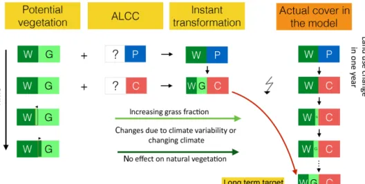
Due to the pasture rule, the history of transitions mat- ters (Reick et al., 2013), especially if the type of land use changes. The so-called potential vegetation is a model internal partitioning of the natural vegetation, which is in accordance with the given climate simulated by MPI-ESM. After anthropogenic land use transitions, the potential vegetation may differ from the actual partitioned natural vegetation, as e.g. grass was transformed to pasture. These differences will smooth out with time, as disturbances (e.g. fire) free land to be converted to the comparatively under-represented part of the potential vegetation. By extreme land use change transitions, as we do apply in our LUC and LUP scenarios within the first model year, the potential vegetation becomes unbalanced to the natural vegetation. Huge transitions within the natural vegetation, which would reflect large changes in the landscape within a short time, are not allowed in JSBACH to counteract against large land use transitions and bring back the partitioning of natural land into equilibrium with the potential vegetation. Therefore the natural vegetation could be out of balance for several decades. To illustrate these effects, a simplified example is shown in Fig. A1, which demon- strates the interplay of the dynamical vegetation, land use, and climate. We start with a climate that favours an equally shared natural vegetation of grass and woody type (potential vegetation). We assume that 50 % of the vegetated area is used for pastoral land use. In accordance with the pasture rule, pastoral land has to be established on grass type vegetation only. If these two pieces of information are com- bined and the potential vegetation plus the ALCC are instan- taneously transformed to the current cover fractions of the grid box, then 50 % of the grid box will be used for pastoral land use. The natural vegetation will shrink by 50 %, and all the grass is taken to establish pasture. So, there is only woody vegetation left after these transitions. The so-called “instanta-

neous transformation” and the current “modelled vegetation”

are the same.

Now, by having an extreme transition from changing all pasture to crops, all managed land will be converted within 1 year, as it is prescribed as an anthropogenic forcing. Assum- ing that the climate is not significantly different to the one of the year before, the potential vegetation stays the same.

Given that cropland covers 50 % of the grid box, and the potential vegetation shares an equal amount of woody and grass cover, the instantaneous transformation of the potential vegetation and the prescribed land use differs from the current partitioning of the natural vegetation, which is covered by woody type only. As JSBACH changes natural vegetation only in small steps, it will take some time to compensate for this misfit. Changes in the natural vegetation due to climate variability, disturbance (e.g. fire), or climate change will alter the natural vegetation, and free land will be used to bring the natural vegetation back to an equilibrium with the potential vegetation (Fig. A1).

In LUC grass gets a strong increase and the woody vegetation shrinks with time to equal out the misfit between instantaneous transformation and “actual cover” (Fig. 6). Because of the former land use, strong transition by converting all pasture to crops leads to this legacy effect. It is the opposite way in the LUP scenario, where woody vegetation is increasing, as crops are changed to pasture and therefore only grass type vegetation is used for land use area. So, woody vegetation, which is sort of hidden in the crop land use, has to build up after all crops are transformed to pasture.

A2 Land use change and harvest within the CMIP5 protocol

The change of land cover is prescribed as transitions from natural to managed land or from one type of land use to an- other type of land use. These are taken from the harmonized land use protocol for CMIP5 (Hurtt et al., 2011), which pro- poses different future pathways for each RCP.

Annual mean harvest data are also taken from the harmonized land use protocol (Hurtt et al., 2011). These yearly values for harvest rates prescribe a certain amount of carbon that has to be taken from the above-ground biomass, which is represented in JSBACH by the sum of three different carbon pools (reserve, green, and woody pool). Weighted by their pool size, the harvest is taken fractionally from these three pools to harvest in total the prescribed value. If this harvest rate is higher than the available biomass, the harvest rate is reduced accordingly. By multiplying the harvest rate with a given factor, we create artificial harvest time series to mimic an intensification of land use (experiments H0.5, H2, H3, H5).

Both the annual transitions and the annual harvest rates are interpolated on a daily timescale and are used as a continuous forcing for MPI-ESM. By doing this, large discontinuities are avoided and harvest is taken continuously.

(10)

Figure A1.Diagram to illustrate the legacy effect of long-term changes in natural vegetation (G: grass; W: woody type) after strong anthropogenic land use transitions (P: pasture; C: crops). Shown are the potential vegetation (model internal) which is in equilibrium with the current climate; the prescribed transition; the instant transformation of the left two pieces of information into a grid cell; and the actual, simulated cover (right column), which accounts for slow changes between two successive years within the natural vegetation.

(11)

Acknowledgements. We acknowledge financial support by the Cluster of Excellence CliSAP (Integrated Climate System Analysis and Prediction, DFG EXC 177/2). We would also like to thank Traute Crüger for her fruitful comments that helped improve the manuscript.

The article processing charges for this open-access publication were covered by the Max Planck Society.

Edited by: P. M. Link

References

Bathiany, S., Claussen, M., and Brovkin, V.: CO₂-induced sahel greening in three CMIP5 Earth System Models, J. Climate, 27, 7163–7184, doi:10.1175/JCLI-D-13-00528.1, 2014.

Boko, M., Niang, I., Nyong, A., Vogel, C., Githeko, A., Medany, M., Osman-Elasha, B., Tabo, R., and Yanda, P.: Africa, in: Africa, Cambridge University Press, Cambridge, UK and New York, NY, USA, 433–467, 2007.

Brovkin, V., Raddatz, T., Reick, C. H., Claussen, M., and Gayler, V.:

Global biogeophysical interactions between forest and climate, Geophys. Res. Lett., 36, L07405, doi:10.1029/2009GL037543, 2009.

Busby, J. W., Cook, K. H., Vizy, E. K., Smith, T. G., and Bekalo, M.: Identifying hot spots of security vulnerability associated with climate change in Africa, Clim. Change, 124, 717–731, doi:10.1007/s10584-014-1142-z, 2014.

Claussen, M.: Modeling bio-geophysical feedback in the African and Indian monsoon region, Clim. Dynam., 13, 247–257, doi:10.1007/s003820050164, 1997.

Giorgetta, M. A., Jungclaus, J., Reick, C. H., Legutke, S., Bader, J., Böttinger, M., Brovkin, V., Crueger, T., Esch, M., Fieg, K., Glushak, K., Gayler, V., Haak, H., Hollweg, H.-D., Ilyina, T., Kinne, S., Kornblueh, L., Matei, D., Mauritsen, T., Mikolajew- icz, U., Mueller, W., Notz, D., Pithan, F., Raddatz, T., Rast, S., Redler, R., Roeckner, E., Schmidt, H., Schnur, R., Segschnei- der, J., Six, K. D., Stockhause, M., Timmreck, C., Wegner, J., Widmann, H., Wieners, K.-H., Claussen, M., Marotzke, J., and Stevens, B.: Climate and carbon cycle changes from 1850 to 2100 in MPI-ESM simulations for the Coupled Model Intercom- parison Project phase 5, J. Adv. Model. Earth Syst., 5, 572–597, doi:10.1002/jame.20038, 2013.

Hurtt, G. C., Chini, L. P., Frolking, S., Betts, R. A., Feddema, J., Fischer, G., Fisk, J. P., Hibbard, K., Houghton, R. A., Jane- tos, A., Jones, C. D., Kindermann, G., Kinoshita, T., Klein Gold- ewijk, K., Riahi, K., Shevliakova, E., Smith, S., Stehfest, E., Thomson, A., Thornton, P., van Vuuren, D. P., and Wang, Y. P.:

Harmonization of land-use scenarios for the period 1500–2100:

600 years of global gridded annual land-use transitions, wood harvest, and resulting secondary lands, Clim. Change, 109, 117–

161, doi:10.1007/s10584-011-0153-2, 2011.

Ilyina, T., Six, K. D., Segschneider, J., Maier-Reimer, E., Li, H., and Núñez Riboni, I.: Global ocean biogeochemistry model HAMOCC: model architecture and performance as component of the MPI-Earth system model in different CMIP5 experimental realizations, J. Adv. Model. Earth Syst., 5, 287–315, doi:10.1029/2012MS000178, 2013.

Jungclaus, J. H., Fischer, N., Haak, H., Lohmann, K., Marotzke, J., Matei, D., Mikolajewicz, U., Notz, D., and Von Storch, J. S.:

Characteristics of the ocean simulations in the Max Planck Insti- tute Ocean Model (MPIOM) the ocean component of the MPI- Earth system model, J. Adv. Model. Earth Syst., 5, 422–446, doi:10.1002/jame.20023, 2013.

Kattge, J., Knorr, W., Raddatz, T., and Wirth, C.: Quantifying photosynthetic capacity and its relationship to leaf nitrogen content for global-scale terrestrial biosphere models, Global Change Biol., 15, 976–991, doi:10.1111/j.1365-2486.2008.01744.x, 2009.

Koster, R., Dirmeyer, P., Guo, Z., and Bonan, G.: Regions of strong coupling between soil moisture and precipitation, Science, 305, 1138–1140, 2004.

Lobell, D. B., Field, C. B., Cahill, K. N., and Bonfils, C.: Impacts of future climate change on California perennial crop yields: Model projections with climate and crop uncertainties, Agr. Forest Meteorol., 141, 208–218, doi:10.1016/j.agrformet.2006.10.006, 2006.

Lobell, D., Cahill, K., and Field, C.: Historical effects of temperature and precipitation on California crop yields, Clim. Change, 81, 187–203, doi:10.1007/s10584-006-9141-3, 2007.

Low, P. S.: Climate Change and Africa, Cambridge University Press, Cambridge, 412 pp., 2005.

Patricola, C. M. and Cook, K. H.: Northern African climate at the end of the twenty-first century: An integrated application of regional and global climate models, Clim. Dynam., 35, 193–212, doi:10.1007/s00382-009-0623-7, 2010.

Pongratz, J., Caldeira, K., Reick, C. H., and Claussen, M.: Coupled climate-carbon simulations indicate minor global effects of wars and epidemics on atmospheric CO₂between AD 800 and 1850, Holocene, 21, 843–851, doi:10.1177/0959683610386981, 2011.

Raddatz, T. J., Reick, C. H., Knorr, W., Kattge, J., Roeckner, E., Schnur, R., Schnitzler, K. G., Wetzel, P., and Jungclaus, J.: Will the tropical land biosphere dominate the climate-carbon cycle feedback during the twenty-first century?, Clim. Dynam., 29, 565–574, doi:10.1007/s00382-007-0247-8, 2007.

Reick, C. H., Raddatz, T., Brovkin, V., and Gayler, V.: Rep- resentation of natural and anthropogenic land cover change in MPI-ESM, J. Adv. Model. Earth Syst., 5, 459–482, doi:10.1002/jame.20022, 2013.

Scheffran, J. and BenDor, T.: Bioenergy and land use: a spatial- agent dynamic model of energy crop production in Illinois, Int.

J. Environ. Pollut., 4–27, doi:10.1002/jame.20038, 2009.

Scheffran, J., Brzoska, M., Kominek, J., Link, P. M., and Schilling, J.: Climate change and violent conflict, Science, 336, 869–71, doi:10.1126/science.1221339, 2012.

Schneck, R., Reick, C. H., and Raddatz, T.: Land contribution to natural CO₂ variability on time scales of centuries, J. Adv.

Model. Earth Syst., 5, 354–365, doi:10.1002/jame.20029, 2013.

Stevens, B., Giorgetta, M., Esch, M., Mauritsen, T., Crueger, T., Rast, S., Salzmann, M., Schmidt, H., Bader, J., Block, K., Brokopf, R., Fast, I., Kinne, S., Kornblueh, L., Lohmann, U., Pin- cus, R., Reichler, T., and Roeckner, E.: Atmospheric component of the MPI-M earth system model: ECHAM6, J. Adv. Model.

Earth Syst., 5, 146–172, doi:10.1002/jame.20015, 2013.

Taylor, C. M., Lambin, E. F., Stephenne, N., Harding, R. J., and Essery, R. L. H.: The influence of land use change on climate in the Sahel, J. Climate, 15, 3615–3629, 2002.

(12)

Vamborg, F. S. E., Brovkin, V., and Claussen, M.: The effect of a dynamic background albedo scheme on Sahel/Sahara precipitation during the mid-Holocene, Clim. Past, 7, 117–131, doi:10.5194/cp-7-117-2011, 2011.

Veron, S., de Abelleyra, D., and Lobell, D.: Impacts of precipitation and temperature on crop yields in the Pampas, Clim. Change, 130, 235–245, doi:10.1007/s10584-015-1350-1, 2015.

Xue, Y. and Shukla, J.: The influence of land surface proper- ties on Sahel climate. Part I: Desertification, doi:10.1175/1520- 0442(1993)006<2232;ATIOLSP>2.0.CO;B2, 1993.

Zeng, N., Neelin, J. D., Lau, K. M., and Tucker, C. J.: Enhancement of interdecadal climate variability in the Sahel by vegetation interaction, Science, 286, 1537–1540, 1999.