A posteriori error analysis for conforming MITC elements for Reissner-Mindlin plates

ELEMENTS FOR REISSNER-MINDLIN PLATES

C. CARSTENSEN^⋆ AND JUN HU^‡

Abstract. This paper establishes a unified a posteriori error estimator for a large class of conforming finite element methods for the Reissner-Mindlin plate problem. The analysis is based on some assumption (H) on the consistency of the reduction integration to avoid shear locking. The reliable and efficient a posteriori error estimator is robust in the sense that the reliability and efficiency constants are independent of the plate thickness t. The presented analysis applies to all conforming MITC elements and all conforming finite element methods without reduced integration from the literature.

1. Introduction

This paper is devoted to the finite element approximation for the Reissner-Mindlin plate problem: Giveng ∈L²(Ω) find (ω,φ)∈W ×Θ:=H₀¹(Ω)×H₀¹(Ω)² with (1.1) a(φ,ψ) + (γ,∇v−ψ)L²(Ω)= (g, v)L²(Ω) for all (v,ψ)∈W ×Θ, and the shear force

(1.2) γ =λt⁻²(∇ω−φ).

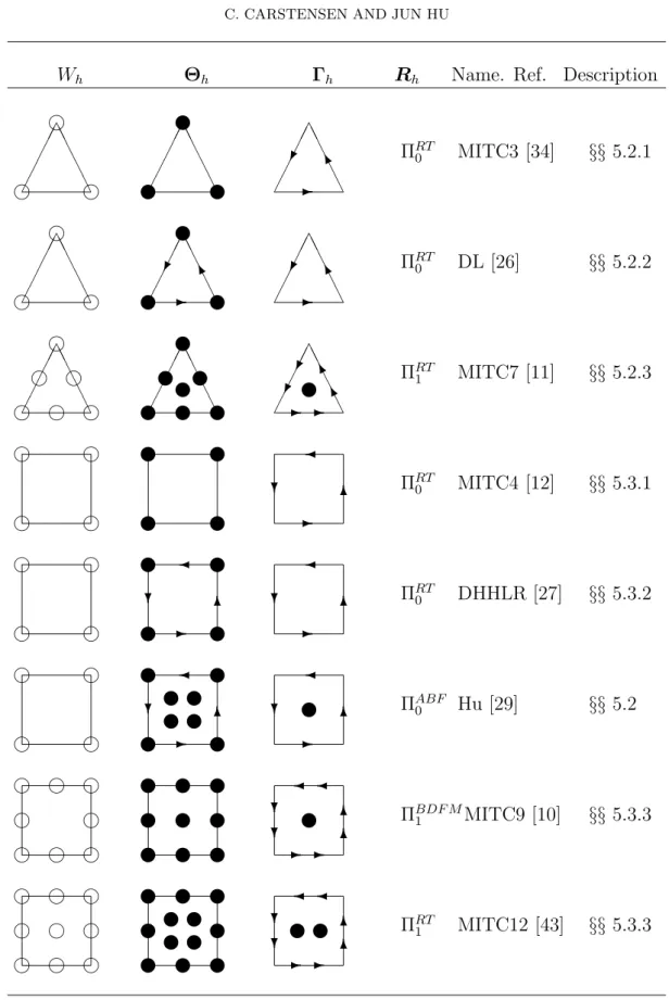
The bilinear form a(·,·) models the linear elastic energy while (·,·)_L²_(Ω) denotes the L² scalar product. Here and throughout this paper, Θ_h ⊂ Θ and Wh ⊂ W denote some finite element spaces over some regular partition Th while R_h denotes the reduction integration operator in the context of shear locking with values in the discrete shear force space Γ_h. Some lower order examples of finite element spaces Wh,Θ_h, and the operator R_h : Θ_h → Γ_h are depicted in Table 1. We refer to Section 5 for further descriptions and for other discrete schemes.

The discrete problem reads: Find (ωh,φ_h)∈Wh×Θ_h with

a(φh,ψ) + (γh,∇v−R_hψ) = (g, v) for all (v,ψ)∈Wh×Θ_h (1.3)

and the discrete shear force

(1.4) γ_h =λt⁻²(∇ω_h−R_hφ_h).

2000 Mathematics Subject Classification. 65N10, 65N15, 35J25.

Key words and phrases. A posteriori, error analysis, Reissner-Mindlin Plate, MITC element AMS Subject Classification: 65N10, 65N15, 35J25.

The first author CC was supported by DFG Research Center MATHEON ”Mathematics for key technologies” in Berlin. The second author JH was partially supported by Natural Science Foundation of China under Grant A10601003.

1

Wh Θ_h Γ_h R_h Name. Ref. Description

AA AA A

h h

h

AA AA A

x x

x

AA AA A -

K Π^RT₀ MITC3 [34] §§ 5.2.1

AA AA A

h h

h

AA AA A

x x

x

- K

AA AA A -

K Π^RT₀ DL [26] §§ 5.2.2

AA AA A

h h

h

h h h

AA AA A

x x

x

x x x

x

AA AA A Kx - - K

Π^RT₁ MITC7 [11] §§ 5.2.3

h h

h h

x x

x x

-

? 6 Π^RT₀ MITC4 [12] §§ 5.3.1

h h

h h

x x

x x

-

? 6

-

? 6 Π^RT₀ DHHLR [27] §§ 5.3.2

h h

h h

x x

x x

x x x x -

? 6 x

-

? 6 Π^ABF₀ Hu [29] §§ 5.2

h h

h h

h h

h h

x x

x x

x x

x

x x x

- - 6

? 6

? Π^{BDF M}₁ MITC9 [10] §§ 5.3.3

h h

h h

h h

h h h

x x

x x

x x

x x x x

x x x x

- - 6

? 6

? Π^RT₁ MITC12 [43] §§ 5.3.3

Table 1. Lower Order Examples of Finite Element Spaces Wh,Θ_h and the Reduction Integration Operator R_h :Θ_h →Γ_h in (1.3)-(1.4) with (H), namely R_hΘ_h ⊂H0(rot,Ω).

This paper aims at aunified reliable and efficient residual-based a posteriori error analysis for a class of conforming elements for the Reissner-Mindlin problem under the hypothesis (H): For anyψ_h ∈Θ_h, there holds

(H) R_hψ_h ∈H₀(rot,Ω),

with the Sobolev spaceH0(rot,Ω) defined in Section 2.1. In fact, (H) is satisfied for all the examples in Table 1 with detailed proofs given in Section 5 below.

With the notation specified below, the main result of this paper implies that the error

kφ−φ_hk²_H¹_(Ω)+kω−ω_hk²_H¹_(Ω)+t²kγ−γ_hk²_L²_(Ω) +t⁴krot(γ−γ_h)k²_L2(Ω)+kγ−γ_hk²_H⁻¹_(Ω) can be controlled by the error estimator

η_h² =: X

E∈E(Ω)

h_E

k[Cε(φ_h)]·ν_Ek²_L²_(E)+ (t²+h²_E)k[γ_h]·ν_Ek²_L²_(E)

+ X

K∈Th

h²_K

kdivCε(φ_h) +γ_hk²_L²_(K)+ (t²+h²_K)kg+ divγ_hk²_L²_(K) +kφh−R_hφ_hk²_H(rot,Ω)+µh(γh)²

up to the data oscillation osc(g). Here and throughout this paper, µh(γh) := sup

ψh∈(S¹₀(Th))²\{0}

(γh,(I−R_h)ψh)_L²_(Ω) kψ_hk_H¹_(Ω) .

The operator C is defined in Subsection 2.1, and the lowest order conforming finite element spaceS₀¹(Th) is defined in Subsection 2.2.

The estimatorηh is robust in the sense that the reliabilty and efficiency constants are independent of the plate thickness t.

Remark 1.1. A different a posteriori error estimate was proposed for the DL el- ement of [26] in [36]. Instead of the norm with the term kγ−γ_hk_H⁻¹_(Ω) here, the term kγ −γ_hkH⁻¹(div,Ω) was analyzed in [36]. It is unsatisfactary that no a priori convergence is known for kγ−γ_hk_H⁻¹_(div,Ω) for conforming MITC methods. This drawback motivated this paper with focuses on kγ−γ_hk_H⁻¹_(Ω). The convergence in this norm is shown, for instance, in[18, Corollary 3.1] and [29, 30] for all examples (except MITC3) of this paper.

Remark 1.2. Compared to the analysis in [36], the analysis in this paper is based on three key arguments: an error representation formula, some mesh dependent norm, and some refined approximation of the Cl´ement-type interpolation operator.

Remark 1.3. The last two terms of ηh concern the consistency error from the reduction integration; they vanish for R_h = I. Hence Theorem 2.1 and 2.2 below apply to any conforming finite element methods without reduction integration.

Remark 1.4. As we shall see in examples of Section 5, µ_h(γ_h) = 0 for high-order (triangle or quadrilateral) schemes. For the lower-order schemes, this term can be

bounded by

µh(γh)² . X

E∈E(Ω)

hE(t²+h²_E)k[γ_h]·νEk²_L2(E)

+ X

K∈T^h

h²_K(t²+h²_K)kg+ divγ_hk²_L²_(K) + h.o.t.

(1.5)

up to computable high-order terms h.o.t.

Here and throughout, an inequality a.b replaces a≤C b with some multiplica- tive mesh-size independent constantC >0 that depends only on the domain Ω and the shape (e.g., through the aspect ratio) of elements (C > 0 is also independent of crucial parameters as the plate thickness t below). Finally, a ≈ b abbreviates a.b.a.

Remark 1.5. For the MITC methods under consideration, one has the following decomposition[18, 29, 30]: There exist unique r∈H₀¹(Ω), α∈H₀(rot,Ω), rh ∈Wh, and α_h ∈Γ_h with

γ =∇r+α, and (∇r,α)L²(Ω)= 0, γ_h =∇r_h+α_h, and (∇r_h,α_h)L²(Ω) = 0.

Therefore, the a priori convergence oft²krot(γ−γ_h)kL²(Ω) is assured by the conver- gence of t²krot(α− α_h)k_L²_(Ω) proved, e.g, in [18, Theorem 3.2] for the MITC7, MITC9 and MITC12 element; cf. [29, 30] for the remaining elements (except MITC3).

Remark 1.6. Although the MITC3 element in Table 1 is unstable in the sense that there is no uniform a priori convergence with respect to the plate thickness t, the estimatorηh is still reliable and efficient. At first glance this might surprise, but is a consequence that an a posteriori error analysis depends on the continuous operators and not on the stability of some discrete scheme.

Other a posteriori error estimators for the finite element methods of the Reissner- Mindlin plate problem can be found in [21, 22, 37]. The paper [21] concerns the nonconforming Arnold-Falk element [4], and the paper [22] works on the stabilized method initialed in [3, 23]. Due to the lacking of the convergence ofkγ−γ_hk_H⁻¹_(div), both frameworks of [22] and [21] are inapplicable herein for the MITC methods. In [37], the authors discuss the a posteriori error estimator for the schemes based on the linked interpolation technique. The result is derived therein under some unproven saturation assumption which our work abandons . In addition, the norm analyzed in that paper contains the term P

K∈Th

(hK +t)⁻²k∇(ω−ωh)−(φ−φ_h)k²_L2(K). The convergence of which is open for the MITC methods without stabilization.

The remaining part of the paper is organized as follows. We first introduce some notations and present main results in Section 2 in detailed forms. The reliability of ηh will be proved in Section 3, with the efficiency in Section 4. In Section 5, we present some examples covered by our analysis, and provide a reliable and efficient computable upper bounds of µh(γh) for them.

2. Notation and Main Results

This section introduces necessary notations and states the main results of this paper.

2.1. Sobolev Spaces and Differential Operators. We use the standard differ- ential operators:

∇r= (∂r/∂x , ∂r/∂y), Curlp= (∂p/∂y ,−∂p/∂x).

The linear Green strain ε(φ) = 1/2[∇φ+∇φ^T] is the symmetric part of gradient field ∇φ. Given any 2D vector function ψ= (ψ₁, ψ₂), its divergence reads divψ =

∂ψ1/∂x+∂ψ2/∂y. With the differential operator rotψ = ∂ψ2/∂x−∂ψ1/∂y for a vector function ψ= (ψ₁, ψ₂), the spaceH₀(rot,Ω) is defined as

H0(rot,Ω) :={v ∈L²(Ω)²|rotv ∈L²(Ω) and v·τ = 0 on ∂Ω}

endowed with the norm

kvk_H(rot,Ω):= kvk²_L²_(Ω)+krotvk²_L²_(Ω)1/2

. The dual space forH0(rot,Ω) reads

H⁻¹(div,Ω) :={v ∈H⁻¹(Ω)²|divv ∈H⁻¹(Ω)}, with the norm

kvk_H⁻¹_(div,Ω) := kvk²_H⁻¹_(Ω)+kdivvk²_H⁻¹_(Ω)1/2

.

We define the following mesh dependent norm, for any (ψ, v)∈H₀¹(Ω)²×H₀¹(Ω), (2.1) |||(ψ, v)|||²_1,h=k∇ψk²_L²_(Ω)+ X

K∈Th

1

t²+h²_Kk∇v−ψk²_L²_(K).

For any functionalF overH₀¹(Ω)²×H₀¹(Ω), we define its dual norm with respect to the norm (2.1) by

(2.2) |||F|||_−1,h= sup

(ψ,v)∈H₀¹(Ω)³\{0}

F(ψ, v)

|||(ψ, v)|||_1,h. The linear operatorC is defined by

Cτ := E

12(1−ν²)[(1−ν)τ +νtr(τ)I]

for all 2×2 symmetric matrices. Here and throughout this paper, t denotes the plate thickness with the shear modulus λ =Eκ/2(1 +ν), the Young’s modulus E, the Poisson ratioν, and the shear correction factorκ. The bilinear form a(φ,ψ) is defined as

a(φ,ψ) = (Cε(φ), ε(ψ))_L²_(Ω) for any φ,ψ ∈Θ:=H₀¹(Ω)² (2.3)

which gives rise to the energy norm

(2.4) kψk²_C :=a(ψ,ψ) for any ψ∈Θ.

2.2. Triangulations and Discrete Spaces. Suppose that the closure Ω is covered exactly by a regular triangulationT_h of Ω into (closed) triangles or quadrilaterals in 2D or other unions of simplices, that is

(2.5) Ω = ∪Th and |K1∩K2|= 0 for K1, K2 ∈ Th with K1 6=K2, where| · |denotes the volume (as well as the length of an edge and the modulus of a vector etc. when there is no real risk of confusion). LetE denote the set of all edges inT_h with E(Ω) the set of interior edges, and N(Ω) the set of interior nodes. The set of edges of the element K is denoted by E(K). By hK we denote the diameter of the element K ∈ T_h. Also, we denote by ωK the union of elements K^′ ∈ T_h that share an edge withK, and by ωE the union of elements having in common the edge E. Given any edgeE ∈ E(Ω) with lengthhE =|E| we assign one fixed unit normal ν_E := (ν₁, ν₂) and tangential vector τ_E := (−ν₂, ν₁). For E on the boundary we choose the unit outward normalν_E =ν to Ω. Onceν_E andτ_E have been fixed onE, in relation toν_E, one defines the elements K₋∈ T_h andK₊ ∈ T_h, withE =K₊∩K₋ and ωE =K+∪K−. Given E ∈ E(Ω) and some R^d-valued function v defined in Ω, with d= 1,2, we denote by [v] := (v|K+)|E −(v|K−)|E the jump ofv across E.

Let ˆK be a reference element. In the case of triangles ˆK := {(ξ, η) ∈ R² : 0 ≤ ξ ≤ 1,0 ≤ η ≤ 1−ξ}, and quadrilaterals ˆK := [−1,1]². The invertable linear (resp. bilinear) transformation ˆK → K is denoted by FK for any triangle (resp.

quadrilateral)K ∈ Th with the Jacobian matrix DFK and its determinant JK. LetS₀¹(Th) denote the lowest order conforming finite element space over Th which reads

S₀¹(T_h) :={v ∈H₀¹(Ω) :∀K ∈ T_h, v|_K◦F_K ∈Q₁( ˆK)}.

Given any non negative integerk, the space Qk(ω) consists of polynomials of total degree at mostk defined over ω in the case ω =K is a triangle whereas it denotes polynomials of degree at mostk in each variable in the case K is a quadrilateral.

With the first order conforming finite element space S₀¹(T_h), we consider the Cl´ement-type interpolation operator or any other regularized conforming finite ele- ment approximation operatorJ :H₀¹(Ω)7→S₀¹(T_h) with the properties

k∇Jϕk_L²_(K)+kh⁻¹_K(ϕ− Jϕ)k_L²_(K) .k∇ϕk_L²_(ωK) and (2.6)

kh^−1/2_E (ϕ− Jϕ)k_L²_(E).k∇ϕk_L²_(ωE)

(2.7)

for allK ∈ T_h, E ∈ E, and ϕ ∈H₀¹(Ω). The existence of such operators is guaran- teed, for instance, in [25, 41, 20, 19].

Giveng ∈L²(Ω), letgh ∈Qk(Th) denote its projection on the (possibly discontin- uous) piecewise polynomial space of degreek with respect to Th. We refer to osc(g) as oscillation ofg

(2.8) osc²(g) := X

K∈Th

(h²_K+t²)h²_K min

gk∈Qk(K)kg−gkk²_L2(K).

2.3. Main Results. The main results concern the reliability and efficiency of ηh. It is stressed thatη_h is the first a posteriori error estimator which estimates an error norm in which a priori convergence is guaranted.

Theorem 2.1. (reliability) Suppose that Θ_h, Wh, Γ_h along with the reduction inte- gration operatorR_h satisfy (H) and(S₀¹(T_h))²Θ_h. Then, the estimator η_h is reliable in the sense that

kφ−φ_hk²_H¹_(Ω)+kω−ωhk²_H¹_(Ω)+t²kγ−γ_hk²_L²_(Ω) +t⁴krot(γ−γ_h)k²_L²_(Ω)+kγ−γ_hk²_H⁻¹_(Ω) .η_h².

Theorem 2.2. (efficiency) Suppose that Θ_h, Wh, Γ_h along with the reduction in- tegration operator R_h satisfy (H) and (S₀¹(T_h))² ⊂ Θ_h. Then, the estimator ηh is efficient such that

η_h² .kφ−φ_hk²_H¹_(Ω)+kω−ωhk²_H¹_(Ω)+t²kγ−γ_hk²_L²_(Ω) +t⁴krot(γ−γ_h)k²_L²_(Ω)+kγ−γ_hk²_H⁻¹_(Ω)+ osc(g)².

3. Proof of Reliability

This section is devoted to the proof of Theorem 2.1 which is divided into six steps.

3.1. Splitting of (I −R_h)φh. Assume with (H) that (Rh −I)φh ∈ H0(rot,Ω).

Then there exist w∈H₀¹(Ω) andβ ∈H₀¹(Ω)² with (Rh−I)φh =∇w−β and (3.1)

kwkH¹(Ω)+kβkH¹(Ω) .k(Rh−I)φhkH(rot,Ω). (3.2)

The proof of (3.1)-(3.2) can be found in Lemma 3.2 of Page 298 of [17].

3.2. Error Representation Formula. The residuals Res₁(·) and Res₂(·) are de- fined by

Res1(v) = (g, v)L²(Ω)−(γh,∇v)L²(Ω) for any v ∈H₀¹(Ω);

Res2(ψ) =−a(φ_h,ψ) + (γh,ψ)L²(Ω) for any ψ ∈H₀¹(Ω)². Notice that (1.1)-(1.3) imply

(γ−γ_h,(R_h−I)φ_h)L²(Ω) = (γ−γ_h,∇w−β)L²(Ω)

= (g, w)L²(Ω)−a(φ,β)−(γh,∇w−β)L²(Ω)

=−a(φ−φ_h,β) + (g, w)L²(Ω)−a(φh,β)−(γh,∇w−β)L²(Ω). Therefore,

kφ−φ_hk²_C+λ⁻¹t²kγ−γ_hk²_L²_(Ω)

=a(φ−φ_h,φ−φ_h) + (γ−γ_h,(∇ω− ∇ω_h)−(φ−φ_h))_L²_(Ω) + (γ−γ_h,(R_h−I)φ_h)L²(Ω)

= Res1(ω−ωh+w) + Res2(φ−φ_h+β)−a(φ−φ_h,β). It follows from the definitions of γ and γ_h and (3.1) that

γ−γ_h =λt⁻²(∇ω− ∇ω_h−φ+R_hφ_h)

=λt⁻²(∇ω− ∇ω_h−φ+φ_h+R_hφ_h−φ_h)

=λt⁻²(∇ω− ∇ωh−φ+φ_h+∇w−β).

Recalling thatkφ−φ_h +βk²_C =a(φ−φ_h+β,φ−φ_h+β), we deduce 1

2kφ−φ_h+βk²_C+1

2kφ−φ_hk²_C+ 1

2λ⁻¹t²kγ−γ_hk²_L²_(Ω) + 1

2 X

K∈Th

λ

t²+h²_Kk∇(ω−ωh+w)−(φ−φ_h+β)k²_L²_(K)

≤ kφ−φ_hk²_C+λ⁻¹t²kγ−γ_hk²_L²_(Ω)+ 1

2kβk²_C+a(φ−φ_h,β)

≤Res1(ω−ωh+w) + Res2(φ−φ_h+β)−a(φ−φ_h,β) + 1

2kβk²_C+a(φ−φ_h,β)

= Res1(ω−ωh+w) + Res2(φ−φ_h+β) +1 2kβk²_C. (3.3)

3.3. Estimate for λ⁻¹t²||rot(γ−γ_h)||. Since

λ⁻¹t²rot(γ−γ_h) =−rot(φ−φ_h)−rot(φ_h−R_hφ_h), there holds

λ⁻¹t²krot(γ−γ_h)k_L²_(Ω) .kφ−φ_hk_H¹_(Ω)+krot(φh−R_hφ_h)k_L²_(Ω). 3.4. Estimate for kγ−γ_hk. For anyψ∈Θ, there holds

(γ−γ_h,ψ)_L²_(Ω) =a(φ−φ_h,ψ)_L²_(Ω)+a(φh,ψ)−(γh,ψ). This proves

(3.4) kγ−γ_hk_H⁻¹_(Ω) .kRes2k_H⁻¹_(Ω)+kφ−φ_hk_H¹_(Ω).

3.5. Abstract a Posteriori Error Estimate. Suppose that Θ_h, Wh, Γ_h along with the reduction integration operator R_h satisfy (H). Then,

kφ−φ_hk²_H¹_(Ω)+kω−ωhk²_H¹_(Ω)+t²kγ−γ_hk²_L²_(Ω) +t⁴krot(γ−γ_h)k²_L²_(Ω)+kγ−γ_hk²_H⁻¹_(Ω)

.|||Res1|||²_−1,h+kRes2k²_H⁻¹_(Ω)+kφh−R_hφ_hk²_H(rot,Ω). (3.5)

In fact, given any 0< ε <1/2, and 0< α <1< t⁻¹, there holds λ⁻¹t²kγ−γ_hk²_L²_(Ω)

=λ(t⁻²−α²)k∇(ω−ωh)−(φ−R_hφ_h)k²_L²_(Ω) +λα² k∇(ω−ω_h)k²_L²_(Ω)+kφ−φ_hk²_L²_(Ω)

+λα²kφ_h−R_hφ_hk²_L2(Ω)+ 2λα²(φ−φ_h,φ_h−R_hφ_h)L²(Ω)

−2λα²(∇(ω−ωh),φ−φ_h)_L²_(Ω)−2λα²(∇(ω−ωh),φ_h−R_hφ_h)_L²_(Ω).

Some Young inequalities prove

λ(t⁻²−α²)k∇(ω−ωh)−(φ−R_hφ_h)k²_L2(Ω)+λα²(1−2ε)k∇(ω−ωh)k²_L2(Ω)

≤λ⁻¹t²kγ−γ_hk²_L²_(Ω)−λα²(1− 2

ε)kφh−R_hφ_hk²_L²_(Ω)

−λα²(1−1

ε −ε)kφ−φ_hk²_L²_(Ω).

An appropriate choice ofαandεand the Korn and Young inequalities, the preceed- ing inequality, (3.3), and (3.2) yield

kφ−φ_hk_H¹_(Ω)+kω−ω_hk_H¹_(Ω)+tkγ−γ_hk_L²_(Ω)

.|||Res1|||_−1,h+kRes2k_H⁻¹_(Ω)+kφ_h−R_hφ_hk_H(rot,Ω). Together with Subsection 3.3 and 3.4 this proves the assertion (3.5).

3.6. Refined Approximation of the Cl´ement Interpolation. Following the idea of [22], we have the refined approximation property for the Cl´ement interpola- tion. Given anyv ∈H₀¹(Ω), set vh =Jv, such that there holds, for anyK ∈ Th and ψ∈H₀¹(Ω)², that

(3.6) h⁻¹_K kv −vhk_L²_(K)+h^−1/2_E kv −vhk_L²_(E).k∇v−ψk_L²_(ωK)+hKk∇ψk_L²_(ωK)

in the sense of Remark 3.1, for any E ⊂ ∂K. To prove (3.6), suppose in the first case that one vertex ofK belongs to the boundary. We assume that the intersection of ∂ωK with ∂Ω contains at least one edge. So a Friedrichs inequality shows

kψk_L²_(ωK) .hKk∇ψk_L²_(ωK). Together with a triangle inequality this yields (3.6).

Remark 3.1. In case ∂ωK does not contain one edge, one can enlarge ωK to ω_K^′ so that ∂ω^′_K contains one edge. Then (3.6) holds for ω_K^′ . The analysis herein is equally valid for this small modification.

In the second case, the vertices ofK are interior nodes and so (v−v_h)|_K remains the same if we change v tov−z for an affine function z onωK when we change vh

accordingly; the Cl´ement approximation operator locally preserves affine functions.

We choose the constant vector A := ∇z as the integral mean of ψ on ωK. As a consequence, (2.6)-(2.7) can be recast as

h⁻¹_K kv−vhk_L²_(K)+h^−1/2_E kv−vhk_L²_(E) .k∇v−Ak_L²_(ωK). Hence a Poincare inequality shows

kψ−Ak_L²_(ωK).hKk∇ψk_L²_(ωK). This concludes the proof of (3.6).

3.7. Proof of Reliability. The proof is based on (3.5)-(3.6) of Subsections 3.5-3.6.

For anyv ∈H₀¹(Ω), letv_h =Jv in (1.3), and ψ∈H₀¹(Ω)² as in Subsection 3.6. An integration by parts shows

Res1(v) = Res1(v−vh). X

K∈Th

h²_K(t²+h²_K)kg+ divγ_hk²_L²_(K)

+ X

E∈E(Ω)

hE(t²+h²_E)k[γ_h]·νEk²_L²_(E)1/2

|||(ψ, v)|||_1,h.

Letψ_h =Jψ with (1.3), then

Res2(ψ) = −a(φh,ψ−ψ_h) + (γh,ψ−ψ_h) + (γh,ψ_h−R_hψ_h). An integration by parts and (2.6)-(2.7) imply

Res2(ψ). X

K∈Th

h²_KkdivCε(φh) +γ_hk²_L2(K)

+ X

E∈E(Ω)

hEk[Cε(φh)]·νEk²_L²_(E)1/2

kψkH¹(Ω)

+ sup

ψh∈(S¹0(Th))²\{0}

(γ_h,(I−R_h)ψ_h)L²(Ω)

kψhk_H¹_(Ω) kψk_H¹_(Ω).

Remark 3.2. In this paper, we use the norm|||Res₁|||_−1,h instead of |||Res₁|||_H⁻¹_(Ω) to get a factor t² +h²_E (Resp. t²+h²_K), which is essential for the efficiency of the estimator in the next section.

4. Efficiency of η

This section is devoted to the proof of the efficiency of ηh from Theorem 2.2. The contributions are analyzed seperately and even locally.

4.1. Efficiency of kg+ divγ_hk. We choose

wK =B_K²(gh+ divγ_h).

Here and throughout this section, gh = Πhg, and BK denotes the standard element bubble function with the following properties [47]:

suppB_K ⊂K, 0≤B_K ≤1, max

x∈K B_K = 1, Z

K

BKdx≈h²_K, and k∇BKk_L²_(K) .h⁻¹_K kBKk_L²_(K). An integration by parts shows

kg_h+ divγ_hk²_L²_(K) . Z

K

(gh+ divγ_h)wKdx dy

= (gh, wK)_L²_(K)−(γh,∇wK)_L²_(K)

= (γ−γ_h,∇wK)_L²_(K)+ (gh−g, wK)_L²_(K).

The sum over all elements leads to X

K∈Th

h²_K(h²_K +t²)kgh+ divγ_hk²_L²_(K) . X

K∈Th

tkγ−γ_hk_L²_(K)th²_Kk∇w_Kk_L²_(K) +kγ−γ_hk_H⁻¹_(Ω)k X

K∈Th

h⁴_K∇w_Kk_H¹_(Ω)

+ X

K∈Th

(h²_k+t²)^1/2h_Kkg_h−gk_L²_(K)kh_K(h²_k+t²)^1/2w_Kk_L²_(K). An elementwise inverse estimate yields

k∇wKk_L²_(K)+hKk∇wKk_H¹_(K) .h⁻¹_K kgh+ divγ_hk_L²_(K). This implies

X

K∈Th

h²_K(h²_K +t²)kg_h+ divγ_hk²_L2(K)

.t²kγ−γ_hk²_L²_(Ω)+kγ−γ_hk²_H⁻¹_(Ω)+ X

K∈Th

(h²_k+t²)h²_Kkgh−gk²_L²_(K). (4.1)

4.2. Efficiency of kdivCε(φh) +γ_hk. Recall BK from the previous section, and set

β_K :=BK(divCε(φ_h) +γ_h).

An integration by parts leads to

kdivCε(φh) +γ_hk²_L²_(K).(divCε(φh) +γ_h,β_K)_L²_(K)

=−(Cε(φ_h), ε(βK))L²(K)+ (γh,β_K)L²(K)

=−(Cε(φh−φ), ε(βK)) + (γh−γ,β_K)L²(K). The arguments of Subsection 4.1 allow the proof of

(4.2) X

K∈Th

h²_KkdivCε(φ_h) +γ_hk²_L²_(K).kφ_h−φk²_H¹_(Ω)+kγ−γ_hk²_H⁻¹_(Ω).

4.3. Efficiency of k[νE ·γ_h]k. Given any interior edge E =∂K+∩∂K−, let bE ∈ H₀²(ωE) denote the edge bubble function from [47], and set

wE =bE[νE·γ_h].

One can prove bE satisfies the following properties suppb_E =ω_E, 0≤b_E ≤1 = max

x∈E b_E, Z

ωE

b_Edx≈h²_E and Z

E

b_Eds≈h_E, (4.3)

k∇bEk_L²_(K±) .h⁻¹_E kbEk_L²_(K±),|∇bE|_H¹_(ωE) .h⁻²_E kbEk_L²_(ωE). (4.4)

For anyE ∈ E(Ω), there holds

k[νE·γ_h]k²_L²_(E).([νE ·γ_h], wE)_L²_(E)

= (divγ_h, wE)L²(ωE)+ (γh,∇w_E)L²(ωE)

= (divγ_h+g, wE)L²(ωE)+ (γh−γ,∇wE)L²(ωE).

The sum over interior edges, the Cauchy inequality plus the shape regularity show X

E∈E(Ω)

h_E(h²_E +t²)k[ν_E ·γ_h]k²_L²_(E)

. X

E∈E(Ω)

(divγ_h+g, h_E(h²_E +t²)w_E)_L²_(ωE)+ (γ_h−γ,∇h_E(h²_E +t²)w_E)_L²_(ωE)

.(X

K∈Th

h²_K(h²_K +t²)kdivγ_h+gk²_L²_(K))^1/2( X

E∈E(Ω)

(h²_E+t²)kw_Ek²_L²_(ωE))^1/2

+kγ_h−γk_H⁻¹_(Ω)k X

E∈E(Ω)

h³_E∇w_Ek_H¹_(Ω)+tkγ_h−γk_L²_(Ω)k X

E∈E(Ω)

thE∇w_Ek_L²_(Ω). The elementwise inverse estimate implies

k∇wEk_L²_(ωE)+hE|∇wE|_H¹_(ωE) .h^−1/2_E k[νE ·γ_h]k_L²_(E). Since P

E∈E(Ω)

h³_E∇wE ∈H₀¹(Ω)², we use the finite overlapping of the supports of∇wE

with E ∈ E(Ω) and the above estimate to derive as k X

E∈E(Ω)

h³_E∇w_Ek²_H¹_(Ω). X

E∈E(Ω)

kh³_E∇w_Ek²_H¹_(ωE) . X

E∈E(Ω)

h³_Ek[ν_E ·γ_h]k²_L²_(E)

≤ X

E∈E(Ω)

hE(t²+h²_E)k[ν_E·γ_h]k²_L²_(E). A similar argument leads to

k X

E∈E(Ω)

thE∇w_Ek²_L²_(Ω) . X

E∈E(Ω)

hE(t²+h²_E)k[ν_E ·γ_h]k²_L²_(E). A patchwise Poincare’s inequality gives

X

E∈E(Ω)

(h²_E+t²)kw_Ek²_L²_(ωE) . X

E∈E(Ω)

(h²_E +t²)h²_Ek∇w_Ek²_L²_(ωE)

. X

E∈E(Ω)

hE(t²+h²_E)k[ν_E ·γ_h]k²_L2(E). A summary of these estimates yields

X

E∈E(Ω)

hE(h²_E +t²)k[ν_E ·γ_h]k²_L2(E)

.t²kγ−γ_hk²_L²_(Ω)+kγ−γ_hk²_H⁻¹_(Ω)+ X

K∈Th

(h²_k+t²)h²_Kkgh−gk²_L²_(K).

Remark 4.1. Note that compared to the usual linear elliptic problem, the edge bubble b_E ∈H²(ω_E) is of high regularity for the proof of the efficiency of k[ν_E ·γ_h]k_L²_(E).

4.4. Efficiency of k[ν_E · Cε(φ_h)]k. For any E ∈ E(Ω), BE ∈ H₀¹(ωE) denote the usual edge bubble function [47] with

suppBE ⊂ωE, 0≤BE ≤1, max

x∈E BE = 1, Z

K±

BEdx≈ Z

ωE

BEdx≈h²_E, Z

E

BEds≈hE, and k∇B_Ek_L²_(ωE).h⁻¹_E kB_Ek_L²_(ωE). Set

β_E =BE[νE · Cε(φh)].

Standard arguments verify

k[νE · Cε(φh)]k²_L²_(E).([νE· Cε(φh)],β_E)E

= (divCε(φh) +γ_h,β_E)L²(ωE)+ (Cε(φh−φ), ε(βE))L²(ωE)

+ (γ−γ_h,β_E)_L²_(ωE).

This, (4.2), and an elementwise inverse estimate yield X

E∈E(Ω)

hEk[ν_E · Cε(φ_h)]k²_L2(E).kγ_h−γk²_H⁻¹_(Ω)+kφ−φ_hk²_H1(Ω).

4.5. Efficieny of kφh−R_hφ_hk and µh(γh). By the definitions ofγ, and γ_h, φ_h−R_hφ_h =−λ⁻¹t²(γ−γ_h)−(φ−φ_h) +∇(ω−ωh).

Therefore,

kφh−R_hφ_hk_H(rot,Ω) .k∇(ω−ωh)k_L²_(Ω)+kφ−φ_hk_H¹_(Ω)+t²krot(γ−γ_h)k_L²_(Ω). We remain to estimate the last term. For anyψ_h ∈(S₀¹(T_h))², there holds

(γh,(I−R_h)ψh) = (γh,ψ_h)−(γh,R_hψ_h)

= (γh−γ,ψ_h) +a(φh−φ,ψ_h)

.(kγ−γ_hk_H⁻¹_(Ω)+kφ−φ_hk_H¹_(Ω))kψhk_H¹_(Ω). Consequently,

sup

ψh∈(S₀¹(Th))²\{0}

(γ_h,(I−R_h)ψ_h)_L²_(Ω)

kψ_hk_H¹_(Ω) .kγ−γ_hk_H⁻¹_(Ω)+kφ−φ_hk_H¹_(Ω). 5. Examples

This section presents a list of examples from Table 1 which allows the computable upper bound for µh(γh), namely

µh(γh)² . X

E∈E(Ω)

hE(h²_E +t²)k[γh]·νEk²_L²_(E)

+ X

K∈Th

h²_K(h²_K +t²)kdivγ_h+gk²_L²_(K)+ h.o.t.

(5.1)