of the Ruperto-Carola University of Heidelberg, Germany for the degree of

Dissertation

submitted to the

Combined Faculties for Natural Sciences and for Mathematics

of the Ruperto-Carola University of Heidelberg, Germany for the degree of

Doctor of Natural Sciences

presented by

Dipl.–Phys. Martin Krause

born in Mannheim, Germany

Oral examination: 15th of May, 2002

On the Interaction of Jets with the Dense Medium

of the

Early Universe

Referees: Prof. Dr. Max Camenzind Prof. Dr. Klaus Meisenheimer

Zusammenfassung

Radiogalaxien wurden in den letzen Jahren bei Rotverschiebungen von ¨uber f¨unf ent- deckt. Sie unterscheiden sich durch h¨ohere Radioleistung und Emissionsliniencharak- teristik von n¨aheren Quellen. Zum Verst¨andnis dieser gasreichen Zentren von Proto- galaxienhaufen wurden hydrodynamische Jets mit K¨uhlung simuliert. Nachdem der dreidimensionale Code Nirvana hierf¨ur getestet und nach Vergleich mit Referenzsim- ulationen als geeignet befunden wurde, wurde eine adiabatische 2D Parameterstudie im relevanten Bereich (Dichtekontrast Jet/Medium η = 10⁻² −10⁻⁵) durchgef¨uhrt.

Dabei wurde eine charackteristische Form und Verbreiterung des Cocoons gefunden.

Die radiale Bugschockausbreitung kann durch eine sph¨arische Druckwelle mit konstan- ter Energiezufuhr analytisch approximiert werden. Die Simulation mit Nichtgleich- gewichtsk¨uhlung zeigte eine Abk¨uhlung des Bugschocks innerhalb der Propagations- zeit auf ≈ 10⁴ K bei ¨außerer Gasdichte von ≈ 1 cm⁻³. Der Bugschock bildete nach einer ersten globalen K¨uhl- und Komprimierungssphase ein großskaliges Absorption- ssystem, das dann fragmentiert und Sterne in typischerweise 10⁴ Kugelsternhaufen zu je 10⁶M bilden k¨onnte. Filamentierung und Fragmentation wurden bei hoher Aufl¨osung best¨atigt. Absorber in fernen Radiogalaxien sowie Kugelsternhaufenexzesse in nahen zentralen Haufengalaxien kann man so erkl¨aren. Mit Literaturparametern f¨ur Cygnus A wurde eine 3D Simulation, erstmals mit Gegenjet, durchgef¨uhrt. Der Bugschock zeigte dabei zwei deutlich getrennte Phasen, die auch in der Beobachtung erkennbar sind. Basisparameter des Jets wurden bestimmt. In der Simulation zeigten sich außerdem charakteristische R¨ontgenstrukturen (Ringe), die in zwei Quellen (M87) identifiziert und interpretiert wurden.

Abstract

In recent years, radio galaxies have been found at redshifts above five. They differ in higher radio power and emission line characteristics from sources nearby. To understand these centers of proto-galaxy-clusters, hydrodynamic jets with cooling were simulated.

After validation of the 3D code NIRVANA by comparison with literature simulations, an adiabatic 2D parameter study in the relevant regime (density contrast jet/medium η = 10⁻² −10⁻⁵) was performed. Characteristic cocoon shape and broadenings were found. The radial expansion can be analytically approximated by a spherical blast wave with constant energy injection. In a non-equilibrium simulation the bow shock cooled to 10⁴ K during jet propagation time (external density 1 cm⁻³). After global cooling and compression, the bow shock turned into a big absorber which fragmented, and should form stars in typically 10⁴globular clusters of 10⁶M. Filamentation and fragmentation was confirmed at high resolution. Absorbers in far-off radio galaxies and globular cluster excesses in nearby CD galaxies can be explained that way. With literature parameters fo Cygnus A, a 3D simulation, for the first time with counter-jet, was performed. The bow shock shows two clearly separated phases, also evident in observation. Basic jet parameters have been derived. The simulation shows characteristic X-ray features (rings) which were identified and interpreted in two sources (M87).

The heavens are telling of the glory of God;

And their expanse is declaring the work of His hands.

Day to day pours forth speech, And night to night reveals knowledge.

There is no speech, nor are there words;

Their voice is not heard.

Psalm 19

Contents

I Introduction 1

I.1 Extragalactic Radio Sources . . . 1

I.1.1 Basic properties of radio galaxies . . . 1

I.1.2 Radio galaxies at high redshift . . . 5

I.2 On the History of Jet Simulations . . . 10

I.3 Aim & Outline . . . 15

I.4 Units & Constants . . . 16

II Numerics 17 II.1 The Magnetohydrodynamic Approximation . . . 17

II.2 The Code NIRVANA CP . . . 17

II.3 Porting to NEC SX-5 Supercomputer . . . 19

II.3.1 Test calculations . . . 19

II.4 Boundary Conditions for the 3D Cylindrical Grid . . . 21

IIIReliability & Convergence 25 III.1 Description of the Codes . . . 26

III.2 Hydrodynamic Jet Simulations . . . 27

III.2.1 Numerical setup . . . 27

III.2.2 Setup A: inter-code comparison of a time series . . . 28

III.2.3 Setup C: the effect of artificial viscosity . . . 30

III.2.4 Setup B: the numerical convergence of a hydrodynamic jet in comparison to K¨ossl and M¨uller (1988) . . . 31

III.3 Magnetohydrodynamic Jet Simulations . . . 38

III.3.1 Configuration . . . 38

III.3.2 Comparison of results . . . 39

III.3.3 Convergence . . . 42

III.4 Discussion . . . 42

IVThe Parameter Space 47 IV.1 Constraints from Observations . . . 47

IV.2 Simulation Study of the Parameter Space . . . 48

IV.2.1 Setup . . . 49

IV.2.2 Results . . . 50

IV.3 Discussion . . . 58

V Simulation with Implicit Cooling 59 V.1 Setup . . . 59

V.2 Results . . . 61

V.3 Comparison to Observations . . . 65

VIBipolar 3D Simulation 69 VI.1 Simulation Setup . . . 70

VI.2 Early Evolution . . . 71

VI.3 Long Term Evolution . . . 73

VI.4 Comparison to Observations . . . 85

VI.4.1 Cygnus A . . . 85

VI.4.2 Abell 2052 . . . 92

VI.4.3 Messier 87 . . . 94

VIIBipolar Jets in 2D with Cooling 97 VII.1Simulation Setup . . . 98

VII.2Run B: High Resolution . . . 99

VII.2.1 Energy distribution . . . 99

VII.2.2 Morphology . . . 102

VII.2.3 Bow shock advancement . . . 105

VII.2.4 State of the gas . . . 105

VII.3Run A: Long Term Evolution . . . 106

VII.4Conclusions . . . 107

VII.5Comparison to observations . . . 108

iii

VIII Summary & Outlook 113

A The Thin Spherical Shell 117

B Publications 121

B.1 Contributions . . . 121 B.2 Refereed Articles . . . 121

C Shortcuts 123

Bibliography 134

Chapter I

Introduction

I.1 Extragalactic Radio Sources

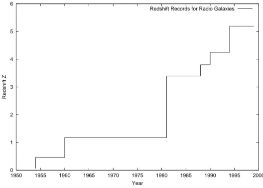
During the last fifty years, radio sources were identified with line emitting ob- jects of ever higher redshift. When Baade and Minkowski (1954) established the redshift of 0.06 for the first time for a radio galaxy (Cygnus A), the main prob- lem for them was optical astrometry. This problem solved, many identifications could be made up to a redshift of about one. In the 1980s it was noticed that the spectral energy distribution of the radio emission steepens with frequency, which gives steeper spectral indices at higher redshift, and that the K-Band infrared luminosity is very well correlated to the redshift. Selecting sources according to these properties caused a considerable jump of the redshift record, with the current record holder TN J0924-2201 at redshift 5.19 (van Breugel et al., 1999) also selected by this method.

I.1.1 Basic properties of radio galaxies

Contemplating the radio image of Cygnus A (Fig. I.1), one notices the basic features of radio galaxies sketched in Fig. I.2:

• central core: Usually, the component with the flattest radio spectrum.

Here resides the active galactic nucleus (AGN). A black hole of millions to a few billions of solar masses is fed here by an accretion disk, accelerating and collimating a wind to velocities close to the speed of light and narrow opening angles: the jet.

• jet beams: A thin beam, sometimes invisible, extending from the core to the hotspots.

• hotspots: One (sometimes more) bright spot on each side of the core.

Here the jet terminates in a prominent shock, called Mach disk. The velocity drops from supersonic to subsonic.

Figure I.1: Radio image of Cygnus A at 5 GHz with 0.4” resolution. (VLA, credit:

NRAO)

• lobes: Large areas around the hotspot, more pronounced on lower fre- quency images, where they can be traced down to the core (Carilli et al., 1991). This is material which passed through the Mach disk. It flows backwards at slower pace than the jet speed. Lobes are often filamentary, have polarisations of more than 40 % and magnetic fields parallel to the well–defined edge of the lobe, at which the intensity rapidly goes to zero.

Only recently, with the launching of the Chandra satellite, detailed views in the X-ray band became available (Fig. I.3). On that picture one can see for the

AGN jet beam

Mach disk hot spot

cocoon = shocked jet matter

expanding shocked external medium contact discontinuity

bow shock

Figure I.2: Sketch of the basic constituents of radio galaxies.

I.1. EXTRAGALACTIC RADIO SOURCES 3

Figure I.3: X-ray image of Cygnus A (Chandra, credit: Chandra Homepage) first time a clear signature of the bow shock. It consists of displaced cluster gas heated to a temperature of 70 mio K (Smith et al., 2002). Eventually, the Mach number of this shock will decrease to one, turning into a sonic disturbance. The bow shock encloses the radio jet.

Objects with one or more of the above properties are classified as Double Radio source Associated with Galactic Nucleus (DRAGN) by Leahy (1993) (see also Leahy, 2000). He also gives more detailed and operational definitions of the phenomenon. However, the definition is not used widely in the astrophys- ical community. Therefore, the term radio galaxy will be used mainly, in the following. A widely accepted distinction among radio galaxies was introduced by Fanaroff and Riley (1974). They divided radio galaxies with two clearly separated hotspots into two classes:

I The separation between the points of peak intensity in the two lobes is smaller than half the largest size of the source.

II The separation between the points of peak intensity in the two lobes is greater than half the largest size of the source.

Fanaroff and Riley (1974) found that nearly all the FR I sources had a lumino- sity less then 2×10³²erg s⁻¹Hz⁻¹sr⁻¹at 178 MHz and with a Hubble constant of 50 km Mpc⁻¹ sec⁻¹, and that the FR II sources were brighter than that. The break may be a function of the optical luminosity of the host galaxy (Owen and White, 1991), which are bright elliptical galaxies. Apart from that, the transi- tion is remarkably sharp. FR I sources are morphologically richer than the FR IIs, and there exist numerous subclassifications (Leahy, 2000). 3C386, 3C84, and 3C338 are representatives of therelaxed doubles, which earned their name from the lack of compact features in the haloes. The different jet morphologies

3C386 3C84 3C338

3C31 3C83.1b 4C35.40

3C296 3C171 3C465

Figure I.4: Several radio morphologies for FR I sources from Leahy (2000).

are often believed to arise by interaction with the external medium. 3C84 is the center of the Perseus cluster of galaxies. Thepeculiarrelaxed double 3C338 is the first ranked member in the Abell 2199 cluster. 3C31, 3C83.1b, 4C35.40, and 3C465 aretailed twin jets. 3C83.1b is a narrow angle tailsource. It is be- lieved that the morphology arises from movement through a cluster atmosphere perpendicular to the jet direction. Thehead tailjet in 4C35.40 is thought to be produced by a movement in jet direction. As usual forwide angle tail sources, 3C465 is the central member of its cluster Abell 2634. The jet bending is in the case of this class thought to arise from winds associated with mergers from clus- ters of galaxies. The isolated radio galaxy 3C296 represents thebridged twin jet

I.1. EXTRAGALACTIC RADIO SOURCES 5 class The bridges are the broad features in the place where you would expect narrow beams in a classical double, like Cygnus A. 3C171 is called a plumed double because of the fuzzy extensions. Such sources are sometimes classified as wide angle tail. Most FR II sources are classical doubles.

I.1.2 Radio galaxies at high redshift

The term high redshift radio galaxy (HZRG) was used, historically, for the highest known redshift sources. By now, it mostly refers to sources with redshift in excess of two (Carilli et al., 2001; van Ojik et al., 1997). In the following the same terminology will be used. For clarity, sources with a redshift upto 0.1 will be labeled low, and the remaining ones intermediate redshift sources. HZRG have been reviewed by McCarthy (1993). But since then, important progress has been made. A more recent comprehensive description can be found in Carilli et al. (2001). More than 150 radio galaxies are now detected at high redshift, half of them within the last three to four years (Carilli et al., 2001). Their redshift corresponds to a cosmological lookback–time of at least 80% the age of the Universe. This observed redshift range also corresponds to the maximum in the redshift distribution of quasars. The spatial density of these objects was at that time about 300 times higher than today.

0 1 2 3 4 5 6

1950 1955 1960 1965 1970 1975 1980 1985 1990 1995 2000

Redshift Z

Year

Redshift Records for Radio Galaxies

Figure I.5: Some redshift records during the last fifty years. References: (Baade and Minkowski, 1954; Minkowski, 1960; Spinrad et al., 1981; Lilly, 1988; Chambers et al., 1990; Lacy et al., 1994; van Breugel et al., 1999)

Spectral Characteristics

Radio galaxies and radio loud quasars, which are thought to be very similar to radio galaxies but seen at smaller viewing angles, with their jets, in general, show four distinct components in their spectrum:

• the infrared–optical–UV continuum of the central source (emission from the accretion disk and its surroundings);

• the radio–optical continuum of the jets (synchrotron emission from rela- tivistic particles in the jet);

• the X–ray and γ continuum (inverse Compton emission from the inner jets);

• narrow and broad emission lines from heated gas.

While these features are shared by all radio galaxies to some extent, certain characteristics show up only at a specific redshift:

Size and power

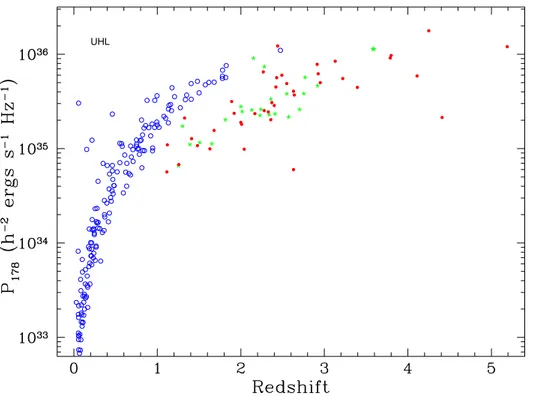
The radio jets themselves show a characteristic length of 100 kpc only at low redshift. HZRG radio jets are typically much shorter (≈ 10 kpc), and less regularly structured. This could possibly be due to a denser environment, where the jet is slower. Alternatively, the HZRG jets could be in a comparatively young state (Blundell and Rawlings, 1999). High redshift radio galaxies are more powerful than their low redshift counterparts. While the only powerful nearby radio galaxy (redshiftz= 0.0562, radio power at 178 MHzP178= 6 10³⁵ erg/sec/Hz) is Cygnus A (Carilli and Barthel, 1996), beyond z ≈ 2 sources with P₁₇₈ > 10³⁶ erg/sec/Hz have been found (Carilli et al., 2001). Assuming a typical spectrum and (unknown) conversion factor of total kinetic jet power to radio power of 10 %, this leads to total kinetic powers of≈10⁴⁶⁻⁴⁷ erg/s for the most powerful sources. Typical extended radio sources in the local universe are one to two orders of magnitude fainter.

Host galaxies

Radio galaxies are hosted by massive ellipticals. At z > 1 they are even two magnitudes brighter in the K band than the brightest non-active galaxies. There is some evidence for a continuous transition, indicating that brighter galaxies host more powerful radio sources (De Breuck et al., 2002). The radio galaxy hosts seem to evolve with redshift (Pentericci et al., 2001): Beyond z = 2.5 HZRG show considerable substructure and clumpiness, indicating interactions and mergers. At z ≈ 2 they appear morphologically relaxed, and down to z ≈ 1 the galaxies approximately double in size. This could indicate that in this redshift range, a large fraction of the stars is produced, and that HZRG are more gas rich than lower redshift radio galaxies.

I.1. EXTRAGALACTIC RADIO SOURCES 7

UHL

Figure I.6: Radio power at a rest-frame frequency of 178 MHz versus redshift for the 3C sample (open circles) and fainter samples from the Leiden group (filled circles and stars), adopted from Carilli et al. (2001).

Emission line lobes

Radio galaxies, in general, show emission line lobes (ELL). The dominant species are usually hydrogen, oxygen, carbon, neon and helium (McCarthy, 1993). High metalicities are observed upto high redshifts (Villar-Mart´ın et al., 2001). Many radio galaxies show line ratios consistent with ionisation by a hid- den central AGN. However, there are some peculiar examples, where it is likely, that the lines are excited by the impact of a bow shock on a dense background medium. According to Meisenheimer and Hippelein (1992), in the intermedi- ate redshift radio galaxy 3C368 (z = 1.13) the bow shock heats the ambient medium to ≈ 10⁷ K. Subsequently, the gas cools down to ≈ 20000 K, where it can be seen in forbidden OII line emission. These ELLs are nicely placed around the radio jet, one side blue, the other redshifted, and lag behind the leading radio feature by about 11 (20) kpc, interpreted as the cooling length.

There are also cases, where both processes significantly contribute (e.g. PKS 2250-41 (z = 0.308), Villar-Mart´ın et al., 1999). Where ionisation by a bow shock is important, this indicates high densities (n≈0.1 cm⁻³, 3C368).

HZRGs show huge halos of Lyman α emitting gas (van Ojik et al., 1996;

R¨ottgering et al., 1996). These halos are much bigger than their low redshift counterparts, extending usually about the same size, or even further out, as the radio source, with up to 10⁹M. Small radio galaxies (<50 kpc) show Lyman

α self absorption (van Ojik et al., 1997; De Breuck et al., 2000), preferentially on the blue wing of the emission line. Associated absorption is also present in small (<50 kpc) radio quasars (Baker, 1999, 2001). Some authors have claimed to see more absorption in high redshift quasars (Ganguly et al., 2001), while others cannot find any redshift dependence (Baker et al., 2001). The discovery of associated absorption means that large amounts of neutral gas have to be present on scales of upto 50 kpc, covering all of the radio source, in almost every small radio loud AGN with a redshift greater than two. Two models have been proposed to explain the observed emission line properties. The first idea was that the the whole region around the radio source is filled with solar system sized clumps (temperature T≈10⁴ K, number density n≈100 cm⁻³), residing in a hot (T≈10⁷ K, n≈0.1 cm⁻³) intra-cluster medium. These clumps would emit lines, when they are illuminated by UV light from a hidden quasar, and produce absorption lines when outside the cone of light. The other model was put forward by Binette et al. (2000). According to their calculations with the photoionisation code MAPPINGS Ic, the absorbing gas is spatially separated and physically distinct from the emission line gas, with very low metalicity (Z

≈0.01Z) and density (n ≈10⁻³cm⁻³).

Also, the total mass of the emission line gas grows strongly with redshift (Baum and McCarthy, 2000), ranging from≈10⁶Mnearby upto≈10¹⁰Mat z≈2. If the kinematics of this gas is dominated by gravitational motions in the majority of cases, as claimed by Baum and McCarthy (2000), than the total (dynamical) mass, including dark matter, would correlate with the gas mass reaching≈10¹⁴Matz= 2. However, many authors take up the position that the velocities of≈1000 km/s in extended emission line regions are probably not of gravitational origin (Sol´orzano-I˜narrea et al., 2001), but rather accelerated by interactions with the radio jet (Sutherland et al., 1993; Villar-Mart´ın et al., 1999).

Alignment effect(s)

In HZRG, the optical continuum is often aligned with the radio emission (Cham- bers et al., 1987; McCarthy, 1993). Polarisation measurements have shown that this emission is highly polarised below z= 1.5 (Carilli et al., 2001). At z >2, less polarisation and, in one case, stellar absorption lines have been found (Dey et al., 1997). The implication is that the aligned continuum is produced by scat- tered light from a hidden quasar at low redshift, with increasing contributions of newly formed stars, possibly triggered by the passage of the jet.

Recently, an alignment was also proposed for the extended X-ray emission (Carilli et al., 2002). While at the time of writing, there was only one HZRG observed with Chandra, and the measurement errors are considerable, the pos- sible implications are interesting: The only extended X-ray emission seen in PKS 1138-262 at z = 2.2 is highly aligned with the radio jet, and probably heated by the bow shock. The unshocked density isn= 0.05 cm⁻³ at 100 kpc from the nucleus and the total mass of hot gas 2.5×10¹²M. The density

I.1. EXTRAGALACTIC RADIO SOURCES 9 is similar to inter-galactic medium (IGM) densities infered from emission line studies (van Ojik et al., 1997), and about a factor of five higher than in Cygnus A, which already resides in a comparatively dense environment.

Environment

It has been argued that the cluster environment of powerful radio galaxies changes substantially with redshift, invoking predominantly rich clusters (or proto-clusters) at higher redshift (Hill and Lilly, 1991; Hill et al., 1993; Best, 2000). New results by McLure and Dunlop (2001) suggest that the comoving space density of clusters at low redshift is almost equal to that of powerful AGN at z ≈ 2.5. Given that in most cases only the dominant, first ranked elliptical develops a powerful AGN, this implies that all the cluster dominant galaxies were active at z = 2.5, and that the powerful radio galaxies at high redshift are located in (proto-) cluster environments. Recently, the environment of HZRG has been searched for Lymanα emitters (Kurk et al., 2001b). The results obtained on two HZRG confirm the above prediction: About 20 objects with spectroscopic redshift have been found around each radio source. At the time of writing this project is still going on.

The nearby Virgo cluster of galaxies with its famous AGN Messier 87 should be a typical example (Camenzind, 1999). The current radio jet is weak, but low frequency radio images show extended emission further out (Klein, 1999), which are interpreted as relics from earlier, recent (≈ 100 million rears old) outbursts. This shows at least that the current (low) activity phase was not the only one in the days of M87. A black hole of three billion solar masses was found at the center of M87. Therefore it is quite plausible that M 87 was much more active in the past.

Dust

Interestingly, the amount of dust in radio galaxies increases with redshift to more than 10⁸M atz= 4, measured from infrared observations (Carilli et al., 2001, and references therein). Measurements of CO emission even imply more than 10¹⁰ solar masses of gas in a few HZRG (Papadopoulos et al., 2001). The presence of large amounts of dust is also implied by the favoured explanation of the continuum alignment effect via scattering by dust grains (McCarthy, 1993).

This is puzzling, since the passage of the radio jet should have easily destroyed dust grains in a short time compared to the radio source age (Villar-Mart´ın et al., 2001; De Young, 1999). As De Young (1998) has calculated in detail, for dust grains to survive the passage of the radio jet, the bow shock has to be slower than ≈ 10,000 km/s or the clouds hosting the dust have to be denser than 1000 cm⁻³. He also points out that rapid cooling behind the bow shock would favour dust survival. If those conditions do not apply, one has to think of other processes, such as dust production by newly formed stars, triggered by the passage of the jet (De Young, 1989).

I.2 On the History of Jet Simulations

Basic model

Jet simulations have been reviewed by Ferrari (1998) and Norman (1993). Two- dimensional simulations started with Rayburn (1977). Norman et al. (1982) introduced the finite difference approach to jet modelling, which is now widely used, also in this work. These simulations, and follow-up work, established the basic model for extragalactic jets (Fig. I.7): A beam is collimated by magnetic forces or external pressure. Within this beam, oblique, crossing shock waves are present. They have a rarefaction zone upstream, and a compression zone downstream, and can move forward and backward through the beam. Each time they reach the jet head, the head gets accelerated by the high pressure region in front of the oblique shocks. Also the collimated jet plasma constantly catches up to the jet head. There it is shocked in the Mach disk, forms a high pressure, hot spot, and is pushed aside, where it flows backwards in a cylinder around the jet beam. The flow gets turbulent, also interacting with oblique shock waves in the beam, and thereby establishing a complex feedback mechanism. This shocked jet plasma is also called cocoon, and was identified with the radio lobes. Because of the supersonic velocity of the hot spot, a bow shock is created in the ambient material, which is separated from the shocked jet plasma by a contact discontinuity.

2D simulations

Norman et al. (1983) then performed a parameter study, and summarised the basics of adiabatic, Newtonian, hydrodynamic jet simulations. The parameter space consists of three dimensions: The ratio of jet to ambient pressure (κ), the ratio of jet to ambient density (η), and the beam Mach number M (ratio of beam velocity to average beam sound speed). As large scale jet beams are not observed to contract or expand by much, the pressure ratio has to be approximately one. This value is used in most jet simulations, and also by Norman et al. (1983). They restricted the Mach number to greater then one because they anticipated 3D effects to be dominant in low Mach number flows.

To the high end there is in principal no limit, but they considered only jets with M < 10. The density contrast was restricted to 0.01 < η < 10. Jets that are denser than that are essentially ballistic. They protrude through the ambient matter almost unaffected, like a solid rod. Lowering the jet density produces more extended cocoons of shocked jet plasma around the jet. Because radio galaxies, in general, show extended synchrotron emitting cocoons, they were identified with, light (η < 1) jets. Jets of young stellar objects do not show such extended cocoons. Therefore, they were identified with heavy (η ≥1) jets.

These results justify that in the following only light jets are considered. The range η < 0.01 was not explored, because those jets propagate very slow, in reality and, even more important, in the computer.

I.2. ON THE HISTORY OF JET SIMULATIONS 11

Kelvin−Helmholtz instability

contact discontinuity

jet

internal shocks

C C

Mach disk

R R RR

backflow

bow shock

turbulence

shocked external medium

cocoon = shocked jet plasma

Figure I.7: Standard jet model. R denotes rarefaction, and C compression zones The advance speed of the jet head can be determined from force balance at the contact discontinuity, in the rest frame of the contact discontinuity. The force from the jet is: [ρj(vj−vcd)²+pj]Aj(see appendix for symbol explanations).

The index j refers to jet values,v_cdis the velocity of the contact discontinuity at the jet head in beam flow direction, which can be equated with bow shock and hot spot velocity. The force from the ambient medium is: [ρmv_cd² +pm]Ahead, where the index m denotes quantities in the ambient medium. A_head is the area of the jet head, across which the contact discontinuity is pushed forward.

This head area is usually larger than the beam area. Its exact amount has to be determined from numerical simulations. Expressing the pressure as p= ρv²/γM² (γ: adiabatic exponent), leads to

vj

v_cd = 1

√η

s1 + 1/γmM_cd

1 + 1/γ_jM_j + 1. (I.1)

is the ratio of beam to head area. For high Mach numbers (I.1) is commonly approximated by

v_cd=v_j

√η

1 +√η. (I.2)

Norman et al. (1983) showed that for heavy jets, is close to one. The heads of light jets expand more, and can reach values as low as 0.1. Since the hydrodynamics of the jet head turns out to be quite complex, was found to be a function of resolution (this thesis, K¨ossl and M¨uller, 1988).

The cocoon broadening can also be estimated analytically (Begelman and Cioffi, 1989; Norman, 1993). Idealising the cocoon as a cylinder with volume V = πr_c²h, given also by its energy E and pressure p, V = (γ −1)E/p, and assuming the distance from core to jet head h to beh=v_headt, with the average head advance speed v_head, and the cocoon energy E to be E = αLt, where L≡πR²_jv_j³/2 is the average kinetic jet luminosity, one can easily calculate the cocoon width (for light supersonic jets, pressure matched with the cocoon):

r_c Rj

= v u u t

αγ(γ −1)M_j²

2√η . (I.3)

This confirms the simulation results of e.g. Norman et al. (1983) that the cocoon grows with Mach number and gets smaller with growing η.

3D simulations

Three-dimensional (3D) simulations (Williams and Gull, 1985; Arnold and Ar- nett, 1986; Cox et al., 1991; Clarke, 1993) have shown that the backflow not only decays into vortices with poloidal velocities, which is observed in the 2D case, but also toroidal (perpendicular to the jet direction) velocities are observed. In general, the cocoon is more complex in 3D. This confirmed the earlier suspicion that the cocoon is turbulent. Because of the limited numerical resolution, the nature of the turbulence could not be studied in detail, so far.

One of the first studied 3D-phenomena was the generation of secondary hot spots. Two mechanisms were proposed that work at different density contrast.

For low density contrast (η <0.05, Norman and Balsara, 1993), the jet beam, jittering around its axis, can be deflected at the contact discontinuity (Williams and Gull, 1985). Because of the high density there, the contact discontinuity moves slowly (I.2), and behaves essentially like a wall. This deflection creates the primary hot spot. Where the contact discontinuity is hit for the second time, a secondary (splatter) hot spot is created. The other model invokes a precessing jet (Cox et al., 1991). Here the primary hot spot is the current working surface, whereas the secondary hot spot is a quickly fading earlier working surface. Both mechanisms work in simulations.

3D hydrodynamical simulations have been used to model various environ- mental conditions. E.g. Norman and Balsara (1993) have calculated a Mach 3.8, η = 0.2 jet with a Mach 1.2 crosswind, a Mach 2,η = 0.02 jet, encounter- ing an oblique Mach 2.8 shock wave, a Mach 4, η = 0.2 jet, encountering an η = 50 cloud, and a Mach 5, η = 0.03 jet, hitting a contact discontinuity at different angles. They could reproduce the morphology of narrow angle tailed radio sources, wide angle tailed radio sources, perpendicularly deflected jets, and splatter hot spots, respectively.

I.2. ON THE HISTORY OF JET SIMULATIONS 13 Magnetic fields

Because jets are detected by their synchrotron emission, they are required to carry magnetic field. For a self-consistent treatment, calculations with the full set of magnetohydrodynamic (MHD) equations are required. The 2D MHD jet simulations fooled the researchers for some time due to a strong axisymmetric effect (Clarke et al., 1986; Lind et al., 1989; K¨ossl et al., 1990b): It was found that for fields of strong magnetic pressure, compared to the thermal pressure, the Lorentz force is able to collimate the shocked jet plasma in front of the Mach disk into anose cone. The nose cone was shown to be unstable in 3D simulation (Clarke, 1993). Already 2D simulations revealed that beam and cocoon can be collimated by a toroidal field, and decollimated by a poloidal field (K¨ossl et al., 1990a). The first result could be confirmed in 3D by Clarke (1993).

He also found that the magnetic field in a jet is, independent of its strength, concentrated in filaments mainly on beam and lobe surface. He attributed this particular arrangement to the velocity shear at those boundaries. These filaments are the ideal locations for reconnection events, producing relativistic particles, which then radiate the synchrotron radiation (Lesch and Birk, 1998).

Synchrotron emission in jets is extended. The lifetime of locally generated relativistic particles (see below) is typically too short to be able to travel to the places where they are observed (Meisenheimer, 1996). Particle reacceleration could take place in those filaments.

Non-thermal ingredients

Magnetic fields are not yet enough for the construction of realistic emission maps. Another important part is the abundance of relativistic particles. These particles are accelerated in reconnection events (see above) and at shocks (Fer- rari, 1998). The transport, shock acceleration and synchrotron cooling of a relativistic electron population carried by a non-relativistic magnetised jet has been studied in 3D by Tregillis et al. (2001). There results show that the termi- nal shock, present most of the time in 2D simulations, dissolves into ashock-web complex. This complex is still a high pressure region. But the beam material can now pass through shocks of varying strength, with a high chance to turn around without passing a shock. Consequently, the simulated radio maps show an extended area around the jet head, where bright emission is found. They confirm that the magnetic field is concentrated in filaments even in the cocoon, where it is generally about an order of magnitude less than in the beam.

Relativistic jets

Another important aspect of jet physics is their high velocity, close to the speed of light, at least close to the AGN. Due to the sophisticated algorithms and the large computational power required, simulations of relativistic jets were carried

out only recently. At the time of writing, no large scale 3D simulation of a magnetised relativistic jet came to the knowledge of the author.

A hydrodynamic relativistic 3D jet has been simulated by Aloy et al. (1999).

One of the most important effects is the relativistic mass increase. This in- creases the effective beam density by Γ², where Γ is the bulk Lorentz factor.

Consequently the η = 0.01,Γ = 7 jet of Aloy et al. (1999) is effectively nearly ballistic, developing only a small cocoon. Furthermore, the jet is more stable than non-relativistic jets, both magnetised and non-magnetised. It is essentially a straight line.

2D simulations of relativistic jets with toroidal field yielded very similar results than the non-relativistic ones, if one takes into account the relativistic mass increase (Komissarov, 1999). 3D simulations have been performed only up to an axial extention of 20 jet radii (Nishikawa et al., 1997, 1998). The preliminary results indicate no spectacular new feature.

Protons or positrons?

So far, it was always assumed that the jet plasma consists of a proton-electron plasma. However, there is no consensus on the nature of the beam material.

Recent developments enabled the inclusion of special equations of state into a relativistic hydrodynamic code. Scheck et al. (2002) simulated a cold baryonic, a hot leptonic, and a cold leptonic jet. The results are strikingly similar, concern- ing morphology and dynamics. Besides a more knotty structure in the synthetic radio map of the hot leptonic jet, the main observational criterion for discern- ing between the different jet ingredients may be the thermal bremsstrahlung emission. While for all models a X-ray cavity is created, because the thin jet material pushes the X-ray atmosphere aside, at energies above 10 MeV the emission from the hot (10¹² K) cocoon begins to dominate over the shell emis- sion in the baryonic and hot leptonic case. Because of the comparatively cold cocoon (10¹¹ K), this is not the case in the leptonic cold jet.

Stability analysis

Besides the numerical study of jets propagating in an undisturbed ambient medium, there has been considerable and increasing interest in the stability properties of jets during the last decade. The main agent of instability and possible destroyer of the jet is the Kelvin-Helmholtz (KH) shear instability.

A fundamental result of its linear analysis (Appl and Camenzind, 1992; Appl, 1996) is that hydrodynamical jets without magnetic field are unstable to KH instabilities of a wide range of wavelengths, while jets with a poloidal field and even more those with a toroidal field in the cocoon (a distribution which is supported by simulation results, see K¨ossl et al. (1990a)) are essentially stable to small wavelength perturbations. Stability increases also with Mach number.

The development of long wavelength instabilities into the nonlinear regime was

I.3. AIM & OUTLINE 15 investigated for the hydrodynamical case in cylindrical and slab symmetry and in three dimensions by Bodo and coworkers (Bodo et al., 1995, 1994, 1998), respectively). They find that the instabilities destroy the jet in a time compar- atively small with respect to the typical lifetime of an astrophysical jet source.

This disruption could be proven to be less severe in the case where the jet is denser than the surrounding medium, when radiative losses are taken into ac- count (Micono et al., 2000, for the three dimensional case), and is even impeded if one includes an equipartition magnetic field (Hardee et al. (1997), three di- mensional, poloidal fields; Rosen et al. (1999), three dimensional, also toroidal fields).

At the time of writing, many interesting jet simulations are still limited by the available computing power. Therefore, it can be expected that progress in computer technology will also advance the simulation of jets and finally the understanding of their physics.

I.3 Aim & Outline

Two fortunate instances had to come together for this project to emerge. At first, the observations of ever higher redshifted radio galaxies showed that these objects are located in comparatively dense environments. Extended emission line regions like e.g. in 3C 368 (Meisenheimer and Hippelein, 1992), gave clear hints that cooling in post-shock regions could be important at least in some cases to produce them. The evidence of shock induced star formation in 4C 41.17 at z= 3.8 (Dey et al., 1997) further supported the idea of dense environments.

On the other hand, the radiation MHD code NIRVANA CP, originally coded by U. Ziegler (Ziegler and Yorke, 1997), and upgraded due to optically thin cooling by M. Thiele (Thiele, 2000) at the Landessternwarte theory group, became ready for use. Consequently, it was decided to use NIRVANA CP to study the propagation of jets into a dense medium, including cooling of that gas.

Simulations of jets had been made with NIRVANA CP only in the proto- stellar regime, so far. Therefore, the reliability of the code, for parameters applicable to extragalactic jets, had to be established, firstly. This has been carried out, and, after a basic description of the methods and the code used in chapter II, which also includes the code adaptation for running on the NEC SX- 5 supercomputer, the results of a comparison of NIRVANA CP recomputations with two refereed simulation results are described in chapter III. Considera- tions about the basic jet parameters for HZRG lead to low density contrasts (η). Therefore, a parameter study was carried out in chapter IV in the region of 10⁻⁵ < η <10⁻². This region was unexplored so far, due to computer power constraints. Next a simulation with time implicit cooling of shocked external material for parameters assumed to be typical for powerful HZRG is presented.

Because the results show that very interesting things happen in the plane of symmetry, the remaining simulations are in bipolar mode: A 3D simulation

with both jets simulated is presented in chapter VI. This simulation was car- ried out for parameters from the literature for the nearby radio galaxy Cygnus A, because recent Chandra observations could identify for the first time the clear shape of the bow shock in this source. The shape of the bow shock turned out to be a good indicator for the underlying physical model assumed. The con- sidered parameters failed to reproduce the Cygnus A bow shock. Nevertheless, by comparison to the model, the conditions in Cygnus A can be constrained.

Cygnus A is an extraordinary source, and can serve as a nearby model for HZRG, in many respects. In chapter VII, again a 2D simulation is presented.

A realistic density profile is used, and cooling is done in a more approximate, time explicit, way. This saves computational resources, gives almost as good results as the implicit version and allows higher resolutions or, at low resolution a long time study of a bipolar jet on a large grid. Both strategies are followed.

The last chapter gives a short summary of the results obtained in this work.

I.4 Units & Constants

The CGS system is widely used in astronomy, and is also applied in this work.

However, for large scale jets there is a typical length scale of 1000 parsec, abbreviated kpc (= 3.0856×10²¹ cm), and a typical time scale of 10⁶ years which is abbreviated by Ma (for Mega-annum, corresponding to 3.156×10¹³ s) in this work. With this typical scale, one can construct a typical velocity:

1 kpc/Ma = 978 km/s. The speed of light in these units is 307 kpc/Ma. Where not stated explicitly, a Hubble constant of 65 km/s/Mpc was used.

Chapter II

Numerics

The numerical computations in this work were carried out with the 3D non- relativistic radiation MHD code NIRVANA CP. The MHD part was coded by U.Ziegler (Ziegler and Yorke, 1997). Optically thin cooling was added by M.Thiele (Thiele, 2000). The code was vectorised with Open-MP like methods, tested and run on the shared memory super-computer NEC-SX5. The results in chapter VI, and partly chapter VII, were obtained on the SX5. The numerics is described in more detail in Thiele (2000) and Ziegler and Yorke (1997).

II.1 The Magnetohydrodynamic Approximation

The study of extragalactic jets in this work is completely based on the assump- tion, that all the plasmas under consideration can be properly described by the theory of magnetohydrodynamics. However, this is only correct, if the charac- teristic scale length (the jet radius≈ kpc) is large compared to the mean free path (Priest, 1994):

λ_mfp≈1 T

10⁹K

2 n cm⁻³

−1

kpc. (II.1)

Since the density in the jet is much lower than 1 cm⁻³ and the temperature can easily exceed 10⁹ K, and can even reach 10¹³ K, this condition is clearly not satisfied. Therefore, one has to assume that the magnetic field provides the coupling between the particles in the jet plasma. In this work, the jet is considered to consist of thermal protons and possibly non-thermal electrons.

The non-thermal electron component is not modeled here. However, for an understanding of the synchrotron emission a self-consistent treatment with a two-component plasma will be necessary. This is beyond the scope of this work.

II.2 The Code NIRVANA CP

The MHD part of NIRVANA CP is identical to the NIRVANA basis and solves the following equations in 3D for density ρ, velocity v, internal energy e, and

magnetic fieldB:

∂ρ

∂t +∇ ·(ρv) = 0 (II.2)

∂ρv

∂t +∇ ·(ρvv) = −∇p+ 1

4π(B· ∇)B− 1

8π∇B² (II.3)

∂e

∂t +∇ ·(ev) = −p∇ ·v (II.4)

∂B

∂t = ∇ ×(v×B), (II.5)

where the pressure p is given by: p = (γ −1)e, with the adiabatic index γ which was assumed to be 5/3 everywhere. NIRVANA can be characterised by the following properties:

1. second order accurate

2. explicit Eulerian time–stepping, 3. operator–splitting formalism,

4. method of characteristics (MOC) / constraint–transport (CT) 5. artificial viscosity

ad 1) Standard finite difference and finite volume methods, similar to ZEUS (Stone and Norman, 1992a,b) were applied. The mesh is staggered, where scalars are defined in the corners and vectors on the center of the surfaces of the cells. The van Leer interpolation method is used, which gives second order accuracy.

ad 2) Explicit Eulerian time–stepping was implemented, with a Courant num- ber of 0.5.

ad 3) Operator–splitting was applied in the advection part. The scheme com- putes the source terms first (−∇p, −∇B²/8π, and −p∇ ·v), then the artificial viscosity (see below), afterwards the magnetic tension part and the induction equation (see below). Finally, the advection is carried out.

ad 4) Magnetic tension ((B· ∇)B/4π) and induction equation (II.5) are treated by a MOC and CT algorithm (Thiele, 2000, and references therein). This method guarantees that the divergence of the magnetic field stays zero, if it was so initially. Alfv´en waves are described correctly.

ad 5) Artificial viscosity terms have been included on the right hand side of momentum (II.3) and energy (II.4) equation. This dissipates high frequency noise and damps overshootings in shock regions, at the cost of smearing the shocks over a few grid cells.

Upgrading to NIRVANA C due to optically thin cooling, Thiele (2000) re- placed equation (II.4) by:

∂e

∂t +∇ ·(ev) =−p∇ ·v− K. (II.6)

II.3. PORTING TO NEC SX-5 SUPERCOMPUTER 19 He also added an additional equation due to generation and depletion of indi- vidual atomic species, with massesm_α, by ionisation and recombination:

∂ρ_α

∂t +∇ ·(ρ_αv) =k_α . (II.7)

K and k_α are computed by the following equations:

K =

N

X

α=0 N

X

β=0

ρα

m_α ρ_β

m_βΛ_{α β} (II.8)

k_α = m_α

N

X

β=0





N

X

γ=β

ρ_β m_β

ρ_γ

m_γIF⁺_{α β γ}−ρ_α ρ_β m_βIF⁻_{α β}



 , (II.9)

where the Λ and IF functions summarise the details of atomic physics and are functions of temperature and, in general, also of the number densities ρ_α/m_α. Λ can also be used to include bremsstrahlung, which was done in chapter V, or cyclotron emission.

II.3 Porting to NEC SX-5 Supercomputer

Part of this work was a further upgrade of the code (to NIRVANA CP) con- sisting in vectorisation and parallelisation for use on a NEC SX-5 computer by OPEN MP like methods, provided by the standard NEC C compiler for this machine. The SX-5 is a shared memory machine. Therefore the changes are moderate. Particularly, no domain decomposition or data transfer between pro- cessors had to be coded, like in the distributed memory case, because all the up to 16 processors have access to the whole memory. The code was revised and fine tuned in order to achieve the maximum possible performance for the given hardware. So far, the code was used with one processor only. A performance of approximately 10⁹ floating point operations per second (FLOPS) was achieved, which corresponds to 25% of the peak performance.

II.3.1 Test calculations

The reliability of the code was tested by computing test problems with the new code version on SX-5 and comparing the result to the output of the old – sufficiently validated – version run on a Linux PC. Since in this work only hydrodynamic calculations were performed on the SX-5 (chapters VI and VII), a hydrodynamic test problem with one species is reported.

The one-dimensional Sod shock problem was computed, which even has a semi-analytic solution (Courant and Friedrichs, 1948). A grid with 4095 cells was used in order to get the maximum possible vectorisation efficiency. This grid was initially divided into two areas. On the left-hand side, density and temperature were set to one, and on the right-hand side they were set to 0.125

Table II.1: Initialisation for Sod Shock Problem Variable Left Hand Side Right Hand Side

ρ 1.0 0.125

T 1.0 0.8

v 0.0 0.0

γ 1.4 1.4

and 0.8, respectively. The velocity was zero, everywhere, and the adiabatic index 1.4.

Due to the ten times higher pressure on the left hand side, a shock wave develops. The computation was carried out both on a Linux PC and on the NEC SX-5 at the High Performance Computing Center in Stuttgart (HLRS).

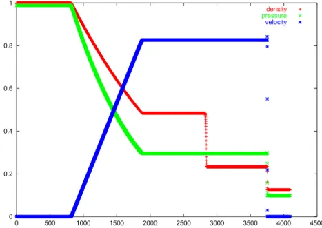
The result after 6000 timesteps and a physical time of 2.3×10⁻⁵ is shown in Fig. II.1 Differences between the two computations could be found only in the velocity in regions where it is close to zero. This velocity differences of the order

∆v≈10⁻¹² should reflect the numerical truncation error. The test calculation also demonstrates the high suitability ofNIRVANA CPin the handling of shock waves. As is shown in Table II.2, a high degree of vectorisation was achieved.

0 0.2 0.4 0.6 0.8 1

0 500 1000 1500 2000 2500 3000 3500 4000 4500

density pressure velocity

Figure II.1: Density, pressure and velocity for the Sod shock test problem after 6000 timesteps, corresponding to a physical time of 2.3 10⁻⁵. The output from the SX-5 computation is plotted, but the output from the PC would be indistinguishable on this graph. The units are normalised in order to fit in the graph, and on the horizontal axis, grid points are indicated.

85% of the user time the code was in vector mode, the vector operation ratio was

II.4. BOUNDARY CONDITIONS FOR THE 3D CYLINDRICAL GRID 21 99.3%, and with the one SX-5 processor used here, a FLOP rate of 1.0 GFLOPS was achieved. This is the expected value, given the maximum performance of 4 GFLOPS, which only can be achieved if the instructions are especially fine tuned. The high vectorisation degree also was indicated by the compiler report:

almost every significant loop was vectorised.

Table II.2: Profile Information for Sod Test

****** Program Information ******

Real Time (sec) : 12.189758 User Time (sec) : 8.827777 Sys Time (sec) : 0.628303 Vector Time (sec): 7.538145 Inst. Count : 306726730 V. Inst. Count : 110947808 V. Element Count: 27955444095 FLOP Count : 8572226294

MOPS : 3188.936809 MFLOPS : 971.051522

A.V. Length : 251.969323 V. Op. Ratio (%): 99.304546

II.4 Boundary Conditions for the 3D Cylindrical Grid

The cylindrical grid is used for a 3D simulation in chapter VI. The disadvantage of the cylindrical coordinates (Z, R, φ) compared to the Cartesian ones is the appearance of internal boundaries. The grid has to be connected somehow over these boundaries. In the φ direction, periodic boundary conditions were applied. In a test problem for the advection part, a pulse could be advected over such a boundary without energy or mass loss. This is only possible because in the advection part of the solver a total variation diminishing (TVD) scheme is applied. For the boundary on the axis, no analogue could be found in the literature. The boundary condition here is similar to the periodic case: One side of the grid should know about the other side. Therefore, three cells were used below the axis, to which consequently the indexi_R= 3 was assigned. With this choice and the staggered mesh, equations (II.2-II.5) are well defined everywhere on the grid. For the scalar quantities, the following boundary conditions were applied:

f(i_Z, j, i_φ) := f(i_Z+i_π,6−j, i_φ) , j= 0,1,2 f(i_Z,3, i_φ) := < f(i_Z,3, i_φ)>|iZ=const,

where iπ denotes the number of grid cells corresponding to the angle π. The last equation indicates that directly on the axis , the scalars were averaged over i_φ for constant i_Z, since all the different i_φ refer to the same physical point.

Due to the staggered mesh, theZ and φ components of vectors are shifted by half a grid cell away from the axis. Therefore for these components, there arise

φ R

grid boundary

initial condition:

jet inflow

ρjetv jetp

jet ρ v p

ext ext ext

grid boundary

Z

Figure II.2: Sketch of the cylindrical grid.

no special problems, and the boundary condition is:

v_{Z, φ}(i_Z, j, i_φ) :=v_{Z, φ}(i_Z+i_π,5−j, i_φ) , j = 0,1,2

The radial vector components are not shifted away from the axis. So, in prin- cipal they all denote the same physical point. However, the flow should be allowed to cross the axis from one side to the other. This is only possible, if the radial velocity takes a reasonable value there. Therefore, two possibilities arise for the boundary conditions:

v_R(i_Z, j, i_φ) := −v_R(i_Z+i_π,6−j, i_φ) , j= 0,1,2 v_R(i_Z,3, i_φ) :=

( 0 : case I

(v_R(i_Z,4, i_φ)−v_R(i_Z,2, i_φ))/2 : case II

In order to check the influence of these two different boundary conditions on the simulation, the jet from chapter VI was simulated twice, the first time with the case I, and the second time with the case II boundary condition. For both runs, the integrated quantities (directionally split energy and momentum, and mass) and also the timesteps were equal. Also, from comparison of the contour plots, no difference could be found. Hence, the flow seems to have enough possibility to flow past the axis, and the detailed behaviour at that line does not influence the result by much. The simulation result also shows, that this approach in general works fine in regions of undisturbed jet flow. Where the jet is dominated by instabilities and wants to bend, the axis looks like an obstacle.

Therefore, the method seems to be problematic if details about the jet beam are of special interest. Nevertheless, the results confirm that the representation of the beam is acceptable, and for the other regions the output was fine. There are severe advantages of the cylindrical grid:

1. Since the jet itself has cylindrical geometry, the required volume for the computational domain is reduced by 1−π/4 ≈22% (for a grid of equal extension in R and positive Z direction).

2. The grid points are naturally concentrated in the area of the jet beam.

This is preferable if no cooling of the external medium is taken into ac- count or if the cooling length there is long.

II.4. BOUNDARY CONDITIONS FOR THE 3D CYLINDRICAL GRID 23 3. There is one special axis (the Z axis) with much more points than the two other directions. This increases the performance for vectorisation, since only inner loops – and therefore one of the directions – are vectorised.

Chapter III

Inter-Code Reliability and Numerical Convergence

The code Nirvana was sufficiently validated concerning MHD test problems (Ziegler and Yorke, 1997) as well as the cooling part (Thiele, 2000). However, the code was not used for the simulation of light extragalactic jets, before. Since also numerical convergence cannot be expected because of computer power lim- itations and the partly turbulent nature of the problem (K¨ossl and M¨uller, 1988), it is not a priori clear how trustworthy individual features are. So, it was decided to test the behaviour of Nirvana in the regime under consideration in comparison to published results, both for the magnetised, and also for the pure hydrodynamic case. It turned out to be of great advantage that one of the reference simulations was a resolution study. So, a statement about the effectiveness of Nirvana compared to other codes could be derived. The resolu- tion study could be extended with Nirvana, resulting in a very high resolution simulation with 400 points per beam radius. This revealed interesting, new, insights especially into the physics of jet boundary layers.

Nirvana and the two codes it is compared to are all second order accu- rate with van Leer interpolation. A hydrodynamic or MHD code constructed after the van Leer scheme is certainly less effective than a code with a piece- wise parabolic method (K¨ossl and M¨uller, 1988; Woodward and Colella, 1984).

Woodward and Colella (1984) showed that besides strong differences in a 1D test problem, the second order accurate codes they tested performed overall equally well in a 2D test, although differences occurred in some details. They note (Woodward and Colella, 1984, p166): Does the accurate representation of a jet in one part of the flow compensate for the presence of noise in another part? So, it really depends on the problem, which code is best suited. For astrophysical jet simulations, there is no comparison of the results of different van Leer scheme codes available, up to now. This study is the first attempt, to the knowledge of the author, to compare the output of different codes in the field of jet simulations, so far. It can be expected that an understanding of the different representations of hydrodynamical features in the different codes will also increase the confidence in jet simulation results in general.

III.1 Description of the Codes

The reference codes are a two dimensional MHD code by Lind (Lind, 1987; Lind et al., 1989), named FLOW, and an also two dimensional HD code by K¨ossl (K¨ossl and M¨uller, 1988), hereafterDKC. A precise description of FLOW can be found only in Lind’s Ph.D. thesis (Lind, 1987). There, Lind points out two special features of FLOW. First, it uses a predictor corrector algorithm for the timestep calculation and second, a specific advection method is applied. This method considers the matter density flux as the primary advective quantity and calculates the remaining fluxes by multiplying the matter density by the specific density in the cell origin. It is not a Godunov scheme, and does not use an exact or approximate Riemann solver. All these codes use explicit Eulerian time stepping. They are second order accurate and use a monotonic upwind differencing scheme. They treat the standard set of ideal (magneto-) hydrody- namic equations (II.2-II.5): Instead of the internal energy e, FLOW and DKC use the total energy u =ρv²/2 +e+B²/8π. Equation (II.4) is then replaced by:

∂u

∂t +∇ ·(uv) =−∇ ·(pv). (III.1)

This is analytically equivalent, but may give different numerical results, in particular in regions of discontinuous flows. Another difference of the codes is the use of artificial viscosity. FLOW has no need for artificial viscosity at all, according to test calculations reported in Lind (1986). DKC and Nirvana use an artificial viscosity in order to enhance the diffusion in regions of strong gradients.

This has the effect that shocks are transported correctly without numerical oscillations at the cost of smoothing the shocks over some grid zones. DKC even makes use of an antidiffusion term, which cancels the effects of artificial viscosity in regions of smooth flow. This point reflects the differences in the details of the implementation of the three codes as summarised in Table III.1.

Table III.1: Differences between the discussed codes FLOW DKC Nirvana

uses e x

uses u x x

art. viscosity x x

antidiffusion x

III.2. HYDRODYNAMIC JET SIMULATIONS 27

III.2 Hydrodynamic Jet Simulations

III.2.1 Numerical setup

As is appropriate for the simulation of axially symmetric jets (normalised) cylin- drical coordinates (r,z) are used. The jet is injected into a homogeneous ambient medium. Density and the pressure there are set to unity. Therefore the sound speed in this external medium is √γ. The jets are injected in pressure equilib- rium and have a density contrast ofη= 0.1 which means that the jet material has 0.1 times the density of the ambient medium. The unit of length is the jet radiusRJ. Velocity is measured in units of ^ppm/ρm, where pm is the pressure andρ_m the density in the ambient medium, and the time unit isR_J/^pp_m/ρ_m. The units were chosen to match the normalised units in Lind et al. (1989) and K¨ossl and M¨uller (1988) as closely as possible. The boundary conditions are rotational symmetry at the jet axis, an outflow condition at the upwind bound- ary for setup A and an impenetrable wall for setup B and C (except for the nozzle). Open boundaries were applied on the two other sides besides setup C where outflow was specified in order to match the original conditions. This should have no noticeable effect, since inflows from those sides are hardly ex- pected. The simulations are carried out at different resolution characterised by the number of grid points the jet beam is resolved with (ppb). Also, higher resolution images than in the original computations are added. Setup A and B recompute the results from K¨ossl and M¨uller (1988), where two simulations with higher resolution were added to setup B, and setup C is designed according to the hydrodynamic jet from Lind et al. (1989). The parameters are summarised in Table III.2. Note the following on the jet nozzle: In the MHD simulations, problems were encountered when the boundary condition was applied in the usual one grid zone only. Therefore the jet values were fixed in an area of four cells from the upwind boundary. In the simulations without magnetic field, the same was done, although it did not influence the results here.

Table III.2: Parameters of the jet models

Setup A B C

Jet velocity v_J 24.5 24.5 25.0

Resolution (ppb) 40 10,20,40,70, 15,30 100,200,400

upwind boundary outflow reflecting reflecting comp. area (in RJ) 8×30 4×10 10×40

reference code DKC DKC FLOW

III.2.2 Setup A: inter-code comparison of a time series

The time evolution of the jet model of setup A is shown in Fig. III.1. The times of the snapshots were chosen very similar to the corresponding model in K¨ossl and M¨uller (1988). Comparing the two computations, at the first glance, one recognises a great similarity: In both cases at early times, a laminar backflow is established, where the terminal Mach disk is nearly perpendicular to the z-axis. At t = 3.18 the laminar backflow phase terminates with the Mach disk becoming oblique and one of the forward and backward moving shocks from the beam extending into the backflow where it decelerates the backflow deflecting it away from the axis. The material to the left of this shock structure at approximately z = 8 at t = 3.89 is pumped off the grid and has disappeared at t= 6.12. The rest of the backflow material essentially stays at its place until the end of the simulation expanding from 2 up to 6 jet radii. Also visible in the simulation are the crossing oblique shock waves in the beam. So far the described features matched the corresponding ones in the

Figure III.1: Contour plots of the density (30 logarithmically spaced lines) for the jet model of setup A. The times for the snapshots were chosen in order to match Fig. 11 of K¨ossl and M¨uller (1988) closely.

original publication very well. In Fig. III.5 the bow shock velocity from this computation is compared to the one in the original publication. It shows a variation on the level of every evaluated timestep with an amplitude of roughly one in the Mach number. This was unrevealed in the original paper due to the lower sampling rate (23 versus 76 snapshots in this computation). The oscillation is modulated by a mode with longer wavelength (represented by the

III.2. HYDRODYNAMIC JET SIMULATIONS 29

Figure III.2: Logarithmic density plot of the jet from setup C. Top: 15 ppb resolution, t=9.76; middle: 15 ppb resolution without artificial viscosity, t=8.94; bottom: 30 ppb resolution, t=10.01

smoothed curve in Fig. III.5) which is about 2 in the present results and 1.7 in K¨ossl and M¨uller (1988). They called this periodic de- and reaccelleration

“beam pumping”. It was interpreted by Massaglia et al. (1996) in the following manner: The oblique shocks have a high pressure on the axis. Each time they arrive at the jet head, the head is accelerated due to this pressure gradient.

Because of this phenomenon multiple bow shocks appear which can be seen in Fig. III.1 (especially at t = 6.12). The overall jet velocity decreases in the laminar phase in a similar way as in the DKC computation. But after t≈4 the decrease in the present computation is faster. Att= 7.73 the jet of the present computation has approachedz = 27.43 which is 9% less than the reference value. At a first glance, it is surprising that the jet velocity decreases at all, for it was derived that the bow shock velocity should be constant (I.2).

For the jet under consideration this bow shock velocity should evaluate to 5.9, approximately achieved in very early times of the simulation. The explanation for this decrease in the bow shock velocity was given by Lind et al. (1989):

As the jet propagates, its head expands and in (I.2) decreases with time. It

Figure III.3: Jets from setup B. 30 logarithmically spaced density contours are shown.

Time and resolution are indicated on top of the individual pictures.

follows that the effective working surface for the jet is ≈ 3RJ at late times of the simulation. This corresponds well to the extent of the jet head in the contour plots (Fig. III.1). A clear discrepancy between the simulations is the appearance of the Kelvin-Helmholtz (KH) instabilities. Where in the original publication only an unstructured bump is visible, in the Nirvana computation a round filigree system with additional instabilities can be seen. The observed differences could be caused by a different effective resolution of the two codes (This question will be examined in more detail in Sect. 3.4). So one can say that the qualitative behaviour of the simulation is well reproduced, which gives additional confidence in the quality of both simulations. But on a quantitative level there are differences. The Nirvana jet is slower at late times and develops a richer cocoon structure. The differences arise in the non-laminar flow phase.

III.2.3 Setup C: the effect of artificial viscosity

The reference paper for this subsection is Lind et al. (1989). They plot their hy- drodynamic jet model at t=10 (in the units used here). This is not possible for