SFB 823
Unreplicated fractional
factorials, analysis with the half-normal plot and
randomization of the run order
Discussion Paper
Joachim Kunert, Adrian Wilk
Nr. 38/2011
Unreplicated fractional factorials, analysis with the half-normal plot and randomization of the run order
Joachim Kunert∗, Adrian Wilk
Fakultät Statistik, Technische Universität Dortmund, 44221 Dortmund, Germany
Abstract: There is an ongoing discussion whether it is wise to randomize the run order of a factorial experiment if there is concern about a possible time trend in the experiment. It can be argued that a randomized order is not very effective because the trend inflates the error. Some authors even criticize that a randomized order will normally not be orthogonal to trend, they claim that therefore there will be bias under the randomized order. On the other hand, a systematic order will only be useful if the true trend is behaving as is predicted by the model.
The present paper investigates the properties of different run order strategies in a simulation study with unreplicated factorial designs. We check to which extend the presence of a time trend might inflate the probability of false rejection of a true null- hypothesis, and we compare the power of significance tests based on the half-normal plot under the various run order concepts.
Keywords: Half-Normal Plot, Randomization, Unreplicated factorial designs, Time trend.
1 Introduction
In the presence of a time trend, the results of an experiment depend on the sequence in which the runs are being carried out. For example, imagine a situation when there is a monotonous time trend and assume that for one factor with two levels all runs of the low level are executed before the runs with the factor at the high level. Then this factor is liable to be declared to have a significant effect on the response variable, even when in reality the factor is not active. This is due to the fact that the effect estimator in this case is highly correlated with the time trend.
To avoid such situations, experimenters may want to use an appropriate run order.
Different strategies exist to deal with a possible time trend. Generally, these can be divided into two basic approaches. Firstly, one might try to avoid a bias due to the time trend, by trying to find a fixed run order which makes the estimators orthogonal or nearly orthogonal to the trend. This approach tries to find an efficient analysis and relies heavily on the appropriateness of some model assumptions. A nice overview of the arguments in favor of a fixed run order is in Mee and Romanova (2010). The second concept randomizes the order in which the runs are performed. This approach tries to derive a valid analysis which depends on model assumptions as little as possible, with the possible disadvantage that the time trend may inflate the variance of the errors. A recent publication supporting this approach for factorial designs is Adekeye and Kunert(2006).
There is an ongoing discussion, which of the two concepts should be applied. The fixed run order is criticized because it might rely too much on model assumptions. If these assumptions should be wrong in a given situation, then the systematic order might lead to strongly biassed results. On the other hand, the randomized run order is criticized because it stresses robustness against model violations too much, at the expense of a possible power loss. Correaet al.(2009) even doubt that a randomized run order can achieve unbiassed estimates. They claim that only
∗Corresponding author: kunert@statistik.tu-dortmund.de
a small fraction of the randomized orders will indeed be orthogonal to a trend. We do not think that this is a valid argument: the correlation with the trend is a random variable under randomization. A random variable can have expectation zero, even if its probability to be zero is negligible. However, as pointed out by Adekeye and Kunert(2006), there is, indeed, no proof that the randomization can validate the assumption that the errors are normally distributed for saturated factorial designs and the analysis with the half-normal plot.
In the present paper, we use a simulation study to compare the performance of a completely randomized run order on the one hand with two systematic run order strategies on the other, one suggested by Cheng and Jacroux (1988) the other by de León Adams et al.(2005) and Correa et al. (2009). We assume that the experiment is done as a saturated fractional factorial design with no degrees of freedom for the estimation of the variance. In such a case, the analysis is often done with the so-called half-normal plot, introduced by Daniel (1959), or variants thereof. We measure the performance of the run-order strategies by the probability of a false rejection and by the power. The probability of a false rejection is compared with the nominal level of significance.
The power is quantified by the probability to identify truly active effects as active effects. We think that any statistical test makes sense only if the probability of a false rejection does not exceed the nominal level - calculating the power of a test which does not keep the nominal level is a fruitless exercise.
In our simulations, we introduce various forms of a time trend to see how the trend influences the performance of the different run-orders. We confine ourselves to analyzing unreplicated (fractional) factorial designs of length n= 8, n = 16 and n = 32 with a saturated model. All factors are at two levels and we assume that all interactions are possibly active. However, we assume that factor sparsity holds, that is, we assume that only a small number of the factors is truly active. Because there are no degrees of freedom for estimation of the variance, the designs are analyzed with the half-normal plot. For all run-orders, we use four different proposals to estimate the error variance and compare these proposals to each other.
The number of runs is denoted byn, the number of contrasts to be estimated in the model by b. We assume that
yi =µ+
b
X
j=1
xijβj+ei, i∈ {1,2, . . . , n},
whereyi is the response at runi,xi= [xi1, . . . , xib]T, with eachxij ∈ {0,1}, is the setting of the design at run i, β = (µ, β1, . . . , βb)T is the vector of parameters andei theith error term. It is supposed that the errors are normally distributed with variance τ2. The mean of the error term, however, is not zero but depends on i, to model a trend.
For the construction of trend resistant designs, it is generally assumed that the trend is linear ini, at times it is assumed to be quadratic. Adekeye and Kunert(2006) presented data from an experiment with a real time trend. This trend was neither linear nor quadratic but followed a less regular pattern. In their paper,Adekeye and Kunert(2006) compared the randomized run order with the trend-free designs constructed by Cheng and Jacroux (1988), assuming a time series model for the trend. The present paper continues this work, using linear and quadratic trends.
This might help the reader to quantify how much can be gained by a systematic run order in ideal situations. Additionally, the present paper also looks at nearly trend-free systematic run orders, proposed by de León Adamset al.(2005) andCorrea et al.(2009).
In each of our simulated designs, a random experiment with valuesv = 1and v =−1, each with probability 1/2, decides on the sign of the trend. We consider linear and quadratic trends.
For linear trends, the ith error term follows a normal distribution with mean v(a·i). Here a describes the intensity, so ei ∼ N(v(a·i), τ2) with 1 ≤ i ≤ n. In the presence of a quadratic trend, the error term follows a normal distribution with mean v(c(i− n+12 )2+a·i). Here the
intensity of the quadratic part of the trend is described byc.
The different concepts of run order are presented in Section 2. Section 3 contains a description of how half-normal plots can be applied. Finally, Section 4 presents our simulation study.
2 Concepts of run order
In Section 4 we compare three different concepts of run order. In what follows the different concepts are shortly presented, only for the case that n= 8 and that we have four factors, but the explanation can be adapted to the other run lengths or numbers of factors.
The designs for all three concepts are constructed by modifying a full factorial design with the desired number of runs. An example for such a design with 8 runs is given in Table 1. Each factor of the experiment is then placed on one of the columns of the full factorial design. In general, it is possible to have up tob=n−1factors in a fractional factorial design. The columns left over, which are not used for factors, will be used for the estimation of interactions. We do not assume that all interactions are negligible. Hence, there will be no degrees of freedom left for the estimation of the variance.
Table 1: 8-run design with standard run order
Run A B C AB AC BC ABC
1 + + + + + + +
2 + + - + - - -
3 + - + - + - -
4 + - - - - + +
5 - + + - - + -
6 - + - - + - +
7 - - + + - - +
8 - - - + + + -
Random run order
Any experimental design with standard run order can be used as a basis for a design with a random run order. Each factor is placed on one of the columns. In general, the columns are selected in such a way that we will have a good resolution of the design. For the design in Table 1, it should make sense to place factor 1 on the column A, 2 on the column B and 3 on C, while factor 4 is placed on the column ABC. This gives a resolution IV design, where the interaction (12) is confounded with (34), (13) is confounded with (24) and (23) is confounded with (14). After selecting the columns, the runs of the design are randomized, i.e. they are permuted with permutationΠ, whereΠis selected strictly at random among alln!possible per- mutations. The design in Table 2 is derived from Table 1 by one random permutation of the rows.
Systematic run order
Experimental designs in which all columns are orthogonal to a linear time trend are con- structed in Cheng and Jacroux (1988). With this approach, only a part of the columns of the design with standard run order can be used. It is not possible to choose a run order where all columns of a complete factorial design are orthogonal to a linear time trend.
An 8-run design with systematic run order is given in Table 3. The columns of the design in Table 3 are orthogonal to a linear time trend. This design has only four columns, so three columns of the design of Table 1 had to be given up. In general with this construction method, a 2k-design looses k columns. In fact, from the full factorial design in standard run order, the
Table 2: Example for a 8-run design with randomized run order (RO)
Run 1 2 3 (12) (13) (23) 4
1 + + - + - - -
2 - - + + - - +
3 - + + - - + -
4 + + + + + + +
5 - - - + + + -
6 - + - - + - +
7 + - + - + - -
8 + - - - - + +
columns allocated with main effects have to be deleted. They are kept free and all effects of interest have to be placed on the remaining columns.
Table 3: 8-run design with systematic run order (SO)
Run 1 2 3 4
1 + + + +
2 + - - -
3 - + - -
4 - - + +
5 - - + -
6 - + - +
7 + - - +
8 + + + -
Run order with minimum bias
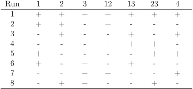
We call the third concept "run order with minimum bias". This was introduced byde León Adams et al.(2005). As opposed to the systematic run order, this concept avoids deleting columns. The columns are as orthogonal to a linear time trend as possible under the restriction that all columns are used. For several run lengths, de León Adams et al. (2005) and Correa et al. (2009) have determined sets of designs, where all columns satisfy the same maximum bias. Furthermore the number of level changes in the factors is as small as possible. In both papers, the reduction of the number of level changes is not relevant for the analysis, it is only introduced to make the experiment easier to carry out. An example is given in Table 4.
Table 4: Example for a 8-run design suggested by de León Adams et al.(2005) (run order with minimum bias)
Run 1 2 3 12 13 23 4
1 + + + + + + +
2 + + - + - - -
3 - + - - + - +
4 - - - + + + -
5 + - - - - + +
6 + - + - + - -
7 - - + + - - +
8 - + + - - + -
In what follows, the following abbreviations are used: RO for randomized run order, SO for systematic run order and MB for run order with minimum bias.
3 Analysis via half-normal plots
For the decision whether an effect is active, an observed test-statistic has to be compared to a critical value. Since we do not have any degrees of freedom left for the estimation of the variance, it is not possible to use a t-test. The half-normal plot makes use of the assumption that most of the effects in the model are zero. Note that the estimators for the not-active effects have expectation zero and hence their absolute value can be used to estimate the variance.
For a fractional factorial design, all estimators βˆj are uncorrelated and have the same variance σ2 =τ2/n. Therefore, the sorted absolute values of the estimatesβˆj are used for an estimate for σ. In our simulations, we consider four different proposals and compare them to each other:
• Proposal 1 (Daniel,1959):
ˆ
σQ=|βˆ|([0.683b+1]),
• Proposal 2 (Lenth,1989):
ˆ σM = 3
2(median|βˆj |),
• Proposal 3 (Lenth,1989):
ˆ
σP SE = 3
2( median
|βˆj|≤2.56ˆσM
|βˆj |),
• Proposal 4 (Dong,1993):
ˆ σASE =
v u u t
1.08 b−z
X
|βˆj|≤2.56ˆσM
βˆj2.
Hereb denotes the number of estimated effects andz is the number of estimates whose absolute value is less than 2.56ˆσM. Kunert(1997) has shown thatσˆP SE has the smallest bias, but σˆASE has the smallest variance among these estimates.
The half-normal plot then uses the test-statistics
|Tj |=|βˆj/ˆσ|,1≤j≤b, whereσˆ is one of these four possibilities.
For the determination of the critical values, the distribution of S :=max
j |Tj |
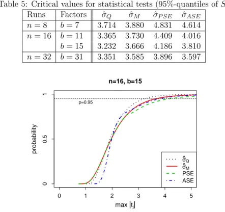
was simulated by 300,000 iterations in the situation where no effect is active. The distribution ofS depends on the number of estimates and therefore on the number of columns of the experimental design which can be used. As a consequence, different critical values have to be determined for the different run order strategies presented in Section 2. In what follows, the critical values used are the simulated 95%-quantiles of the distributions ofS. Some relevant critical values are given in Table 5. HenceC(b, α)denotes the (1-α)-quantile of the distribution ofS in the presence ofb columns. The distributions of the four variants are illustrated forn= 16withb= 15in Figure 1.
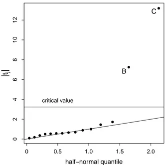
Finally an example for a half-normal plot is given in Figure 2.
Table 5: Critical values for statistical tests (95%-quantiles ofS) Runs Factors σˆQ σˆM σˆP SE σˆASE
n= 8 b= 7 3.714 3.880 4.831 4.614 n= 16 b= 11 3.365 3.730 4.409 4.016 b= 15 3.232 3.666 4.186 3.810 n= 32 b= 31 3.351 3.585 3.896 3.597
n=16, b=15
max |tj|
probability
p=0.95
σ^ σ^Q M
PSE ASE
0 1 2 3 4 5
00.51
Figure 1: Distribution of S under no trend for n = 16 and b = 15. The intersections with
’p=0.95’ lead to critical values for statistical tests.
4 Simulation study
In this section the performances of the three strategies of run order introduced in Section 2 are investigated in a simulation study.
In a first step, we restrict the analysis to the randomized run order and large linear trends.
We consider the three run lengths 8, 16 and 32. This step is done to determine the robustness of the randomized run order: Can a randomized run order truly avoid bias due to a time trend?
In the second part of the simulation study, all concepts are researched in the situation of linear and quadratic trends. Here, we consider only the run length 16. In this part, we will compare the power loss of the three strategies in the presence of a moderate linear trend and we will compare the robustness of the three strategies to the presence of non-linear trends.
We use two criteria to evaluate the three strategies. The first one is the probability of false rejection (PFR):
P F R=P(max
j |Tj |> C(b, α)).
It gives the proportion of designs where at least one effect is declared as active, although in reality all effects are not active. This proportion is simulated in the presence of time trends with different intensities. Hence, PFR determines whether statistical tests keep the nominal level of significance under the various strategies of run-orders.
The second criterion is the probability of effect detection (PED):
P ED=P( min
j:βj6=0|Tj |> C(b, α)).
The probability of effect detection describes the proportion of designs, where all truly active effects are identified as active.
● ●● ● ● ● ● ● ● ● ●
● ●
●
●
half−normal quantile
|tj|
critical value
0 0.5 1.0 1.5 2.0
024681012
C
B
Figure 2: Example of a HNP whereσˆQ is used to estimate the error variance. Here effects B and C would be declared as active.
The simulation study is organized as follows.
Procedure 1: Determination of PFR
(1) RO: Permute the rows of the design with standard run order.
SO: Permute the columns of the design with systematic run order.
MB: Choose at random one design out of the set of feasible designs in the catalog in de León Adamset al. (2005). Permute the columns of the chosen design.
(2) Create the data by equation yi=ei. (3) Compute the test statistic max|tj |.
(4) Repeat step 1 to 3, until 100,000 designs have been derived.
(5) For all three strategies and all four variants compute the respective proportion of designs where the test statistic exceeds the critical valueC(b, α). This proportion is an estimation for the probability of false rejection.
Procedure 2: Determination of PED
(1) RO: Permute the rows of the design with standard run order.
SO: Permute the columns of the design with systematic run order.
MB: Choose at random one design out of the set of feasible designs in the catalog in de León Adamset al. (2005). Permute the columns of the chosen design.
(2) Create the data by equation yi=µ+Pb
j=1xijβj+ei. (3) Compute the test statistic tj.
(4) Check whether all active effects are identified as active effects, i.e. |tj |> C(b, α) for all j withβj 6= 0.
(5) Repeat step 1 to 4, until 100,000 designs have been derived.
(6) Compute for all three strategies and all four variants the respective proportion of designs where the condition in step 4 is achieved. This proportion is an estimation for the proba- bility of effect detection.
Note that the columns are randomized for two of the strategies. The reason is that, in general, the correlation between the columns and the trend varies between the columns.
The first part of the simulation only deals with the randomized run order, with run lengths n = 8, n = 16 and n = 32. It only considers the scenario that there are no active factors and there is a large linear trend. The distribution of the largest contrast in the presence of the trend is then compared to the distribution that we have already derived under normally distributed errors in Section 3.
The observations in the presence of a large linear trend are simulated in the following way.
The variance of the error is set equal to zero. Furthermore no effect is active and the size of the trend, a, is set to 1. Note that a can be chosen arbitrarily, because the trend is a linear component in numerator and denominator of the test statistic. This corresponds to the limiting case that the error variance is arbitrary and the trend converges to infinity. It should be the worst case for the randomized order in the presence of a time trend, because the bias according to de León Adamset al.(2005) then converges to infinity. As the nominal level is set to5%, the proportion of designs that leads to a false rejection of the null hypothesis should be five percent.
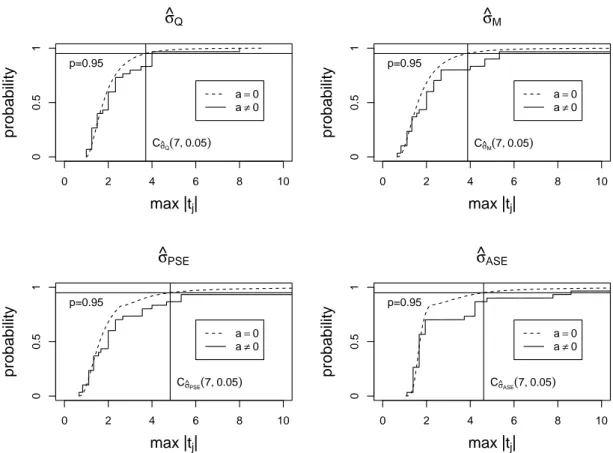
However, we observe for the small design with n= 8, in the presence of a large trend, that the largest contrast gets declared active in at least 13 percent of the cases, see Table 6. This result is also demonstrated in Figure 3 where the distribution under ideal conditions and the distribution under trend are plotted together. Obviously, the distribution under the large trend is discrete, it is far from the continuous distribution derived under normality. Hence, the randomized order does not guarantee keeping the nominal level in the presence of a linear trend for factorial designs of size 8! (This was already observed byAdekeye and Kunert (2006).)
Fortunately, this problem disappears for larger designs, when the two distributions become much more similar, see Figures 4 and 5. Here, the nominal levels are only minimally exceeded, with PFR equal to7.6%in the maximum, see Table 6.
This indicates that, if we do an analysis with the half-normal plot, then randomization of the run-order does indeed help keeping the nominal level in the presence of a linear time trend - provided we have 16 runs or more.
Table 6: PFR of randomized run orders, strong linear trend,α= 0.05 Runs Factors σˆQ σˆM σˆP SE σˆASE
n=8 b=7 0.165 0.199 0.135 0.133 n=16 b=15 0.076 0.072 0.062 0.075 n=32 b=31 0.063 0.063 0.061 0.065
In the second part of the study, we consider all three design strategies, but we restrict to the case of a 16 run design. For this case, we simulate various scenarios. The first scenario assumes that there is no active effect and tries to simulate a moderate time trend.
σ^
Q
max |tj|
probability
a=0 a≠0 Cσ^Q(7, 0.05) p=0.95
0 2 4 6 8 10
00.51
σ^
M
max |tj|
probability
a=0 a≠0 Cσ^M(7, 0.05) p=0.95
0 2 4 6 8 10
00.51
σ^
PSE
max |tj|
probability
a=0 a≠0 Cσ^PSE(7, 0.05) p=0.95
0 2 4 6 8 10
00.51
σ^
ASE
max |tj|
probability
a=0 a≠0 Cσ^ASE(7, 0.05) p=0.95
0 2 4 6 8 10
00.51
Figure 3: Distribution of max|Tj |(n= 8, randomized run order, no active effects): Comparison of the distribution when i) there is no trend (a= 0) to the distribution when ii) the trend becomes infinitely large (a6= 0).
We make use of the fact that, if a variableZ is standard normal,Z ∼N(0,1), then E(|Z |) =
r2 π.
If there is no trend and there are no active factors, then we will have for Y1−Yn, the difference between the first and the last observation, thatY1−Yn∼N(0,2σ2). Hence,
E(|Y1−Yn|) =√ 2σ
r2 π =
r4 πσ.
This implies for our simulations that, if we setσ = 1and the trend intensityaequal toa= 151 q4
π, then the expected difference between the first and 16th observation caused by the trend will be just as large as the expected difference caused by the random noise.
In this scenario, we observe that all three concepts appear to perform well, the nominal levels are approximately kept, see Table 7.
These results show that for all three design strategies a moderate linear trend does not destroy the nominal level of the half normal plot, if the design is large enough. Thus, all three strategies appear to provide valid tests in the presence of a linear trend.
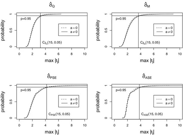
In the next scenarios we compare the power of the concepts. In these settings we assume that the response of the 16-run design is influenced by one active effect of size β1 = 1. When
σ^
Q
max |tj|
probability
a=0 a≠0 Cσ^Q(15, 0.05)
p=0.95
0 2 4 6 8 10
00.51
σ^
M
max |tj|
probability
a=0 a≠0 Cσ^M(15, 0.05) p=0.95
0 2 4 6 8 10
00.51
σ^
PSE
max |tj|
probability
a=0 a≠0
CPSE(15, 0.05) p=0.95
0 2 4 6 8 10
00.51
σ^
ASE
max |tj|
probability
a=0 a≠0
CASE(15, 0.05) p=0.95
0 2 4 6 8 10
00.51
Figure 4: Distribution of max|Tj |(n= 16, randomized run order, no active effects): Compar- ison of the distribution when i) there is no trend (a= 0) to the distribution when ii) the trend becomes infinitely large (a6= 0).
Table 7: PFR of all concepts, linear trend (moderate),α= 0.05, n=16
RO SO MB
no trend 0.05 0.05 0.05 linear trend 0.05 0.05 0.05
we then simulate the moderate trend as before, it appears that all concepts perform similarly.
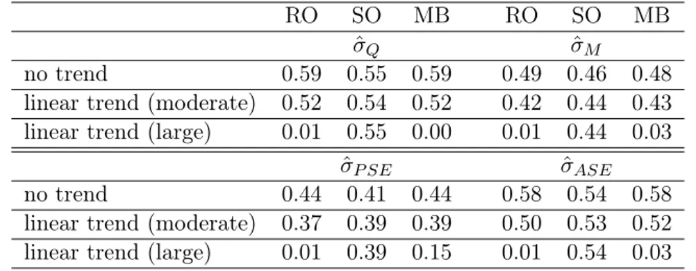
The power of the randomized order is only slightly smaller. It should be noted, however, that the trend-free run order has a slightly lower power in a further scenario, where we assume that the trend is not present. This is due to the fact that the trend-free run order can only use a smaller number of columns. On the other hand, when we simulated the trend as large, then both the randomized run order and the run order with minimum bias experienced a dramatic loss of power, see Table 8.
As an aside, when comparing the four estimates of the variance for any given design, then in general the estimators σˆQ andσˆASE lead to the highest power.
In our last scenario, we consider a quadratic trend instead of the linear one. For this scenario, the trend parameters are set to a= 0 and c = 0.1. Here we observe that only the randomized run order is able to provide a valid test that keeps the nominal level, see Table 9.
Hence, we derive from our simulations the following message: The two systematic run orders considered here, have the problem that they only work properly if the trend is truly linear. In the presence of a non-linear trend, they may fail dramatically. The randomized run order appears
σ^
Q
max |tj|
probability
a=0 a≠0 Cσ^Q(31, 0.05) p=0.95
0 2 4 6 8 10
00.51
σ^
M
max |tj|
probability
a=0 a≠0 Cσ^M(31, 0.05) p=0.95
0 2 4 6 8 10
00.51
σ^
PSE
max |tj|
probability
a=0 a≠0
CPSE(31, 0.05) p=0.95
0 2 4 6 8 10
00.51
σ^
ASE
max |tj|
probability
a=0 a≠0
CASE(31, 0.05) p=0.95
0 2 4 6 8 10
00.51
Figure 5: Distribution of max|Tj |(n= 32, randomized run order, no active effects): Compar- ison of the distribution when i) there is no trend (a= 0) to the distribution when ii) the trend becomes infinitely large (a6= 0).
to provide a valid test; it may, however, loose power if the trend gets too large.
Acknowledgment
Financial support of the Deutsche Forschungsgemeinschaft (SFB 823 "Statistical modelling of nonlinear dynamic processes", Project B2: "Characterization of the dynamical process of the incremental sheet metal forming") is gratefully acknowledged. Part of the research was done while the first author was Visiting Fellow of the Isaac Newton Institute for Mathematical Sciences, University of Cambridge.
Table 8: PED of all concepts, linear trend (moderate/large),α= 0.05, n=16
RO SO MB RO SO MB
ˆ
σQ σˆM
no trend 0.59 0.55 0.59 0.49 0.46 0.48
linear trend (moderate) 0.52 0.54 0.52 0.42 0.44 0.43 linear trend (large) 0.01 0.55 0.00 0.01 0.44 0.03
ˆ
σP SE ˆσASE
no trend 0.44 0.41 0.44 0.58 0.54 0.58
linear trend (moderate) 0.37 0.39 0.39 0.50 0.53 0.52 linear trend (large) 0.01 0.39 0.15 0.01 0.54 0.03
Table 9: PFR of randomized run orders, quadratic trend, α= 0.05, n=16
RO SO MB RO SO MB
ˆ
σQ σˆM
quadratic trend 0.06 0.64 0.34 0.06 0.57 0.32 ˆ
σP SE σˆASE
quadratic trend 0.06 0.52 0.33 0.06 0.60 0.36
References
Adekeye, K. and Kunert, J. (2006). On the comparison of run orders of unreplicated2k−p designs in the presence of a time trend. Metrika,63, 257–269.
Cheng, C. and Jacroux, M. (1988). The Construction of Trend-Free Run Orders of Two-Level Factorial Designs. Journal of the American Statistical Association,83, 1152–1158.
Correa, A., Grima, P., and Tort-Martorell, X. (2009). Experimentation order with good proper- ties for2k factorial designs. Journal of Applied Statistics,36, 743–754.
Daniel, C. (1959). Use of Half-Normal Plots in Interpreting Factorial Two-Level Experiments.
Technometrics,1, 311–341.
de León Adams, G., Grima, P., and Tort-Martorell, X. (2005). Experimentation Order in Facto- rial Designs with 8 or 16 Runs. Journal of Applied Statistics,32, 297–313.
Dong, F. (1993). On the Identification of Active Contrasts in Unreplicated Fractional Factorials.
Statistica Sinica,3, 209–217.
Kunert, J. (1997). Use of the factor sparsity assumption to get an estimate of variance in industrial experiments with many factors. Technometrics,39, 81–90.
Lenth, R. (1989). Quick and Easy Analysis of Unreplicated Factorials. Technometrics, 31, 469–473.
Mee, R. and Romanova, A. (2010). Constructing and Analyzing Two-Level Trend-Robust De- signs. Quality Engineering,22, 306–316.