Time-optimal nonlinear model predictive control

Time-Optimal Nonlinear Model Predictive Control

Direct Transcription Methods with Variable Discretization and Structural Sparsity Exploitation

DISSERTATION

submitted in partial fulfillment of the requirements for the degree

Doktor-Ingenieur (Doctor of Engineering)

in the

Faculty of Electrical Engineering and Information Technology at Technische Universität Dortmund

by

Christoph Rösmann, M.Sc.

Münster, Germany

Date of submission: April 29, 2019

Place of submission: Dortmund, Germany

First examiner: Univ.-Prof. Dr.-Ing. Prof. h.c. Dr. h.c. Torsten Bertram Second examiner: Univ.-Prof. Dr.-Ing. Martin Mönnigmann

Date of approval: October 14, 2019

Preface

This thesis was written during my work at the Institute of Control Theory and Systems Engineering of the Faculty of Electrical Engineering and Information Technology at the Technical University of Dortmund.

I would like to thank Univ.-Prof. Dr.-Ing. Prof. h.c. Dr. h.c. Torsten Bertram that he made my scientific work possible and generously supported it. I am very grateful for his valuable feedback, confidence and inspiring suggestions. He has always given me the freedom to develop my own scientific knowledge and present it to a broad audience at numerous local and international conferences. I would also like to thank Univ.-Prof. Dr.-Ing. Martin Mönnigmann, who agreed to review my thesis as second examiner. I greatly appreciate his valuable feedback and expertise.

Additionally, I would like to thank all staff members and former staff members of the Institute of Control Theory and Systems Engineering for the pleasant working atmosphere, the cooperativeness and camaraderie. In particular, I am grateful for the assistance given by apl. Prof. Dr. rer. nat. Frank Hoffmann. His excellent experience in many different engineering and scientific fields, his insightful comments and the intensive discussions have helped me a lot to advance my ideas and research projects.

Dr.-Ing. Daniel Schauten deserves my special thanks for the many valuable conver- sations, advices and support during my time at the department, especially regarding best practices in teaching and research. I am very thankful to Artemi Makarow for all the time we spent discussing and questioning many control theoretical topics, for the conference trips we have experienced together and for the extraordinary support and encouragement especially in the final stages of completing my thesis. Special thanks also go to Maximilian Krämer and Christian Wissing for the intensive ex- change in many topics, especially in robotics and software development in C++. For the always kind assistance with administrative and technical questions I would like to thank Nicole Czerwinski, Gabriele Rebbe, Sascha Kersting, Jürgen Limhoff and Rainer Müller-Burtscheid.

I would also like to express my gratitude for the financial support provided by the German Research Foundation (DFG).

Words of gratitude are dedicated to my friends who helped me to find distraction and relaxation. Finally, I am very grateful to my family for their continuous unconditional support and encouragement throughout my life.

Dortmund, October 2019 Christoph Rösmann

Abstract

This thesis deals with the development and analysis of novel time-optimal model pre- dictive control concepts for nonlinear systems. Common realizations of model predic- tive controllers apply direct transcription methods to first discretize and then optimize the subordinate optimal control problems. The key idea of the proposed concepts is to introduce discretization grids in which the underlying discretization is explicitly treated as temporally variable during optimization. A single optimization parameter for all grid intervals leads to the global uniform grid, while the definition of an indi- vidual parameter for each interval results in the local uniform and quasi-uniform grid representations. The proposed grids are well-suited for established direct transcription methods such as multiple shooting and collocation. In addition, a proposed non-uni- form grid with extended multiple shooting is highly beneficial for bang-singular-bang control systems with simple constraint sets. The minimization of the local time in- formation of a grid leads to an overall time-optimal transition. Integration with state feedback does not immediately guarantee asymptotic stability and recursive feasibility.

To this end, the thesis provides a grid adaptation scheme capable of ensuring practi- cal stability and, under more restricted conditions, also nominal asymptotic stability while maintaining feasibility. The practical stability results facilitate the systematic dual-mode control design that restores asymptotic stability and establishes smooth stabilization.

The secondary objective of this thesis is the computationally efficient realization of time-optimal model predictive control by exploiting the inherent sparse structures in the optimal control problems. In particular, the efficient computation of first- and second-order derivatives required for iterative optimization is facilitated by a so-called hypergraph. The hypergraph captures the structure of the transcribed optimal con- trol problems and enables an almost linear relation between computation time and grid size. In addition, the hypergraph shows negligible computation times for each reconfiguration that is essential for grid adaptation.

Numerous examples in simulation and with a real experimental system demonstrate the capabilities and potentials of the proposed concepts. Extensive benchmarks in C++ compare the proposed methods with each other and the current state of the art.

The methods based on variable discretization outperform the current time-optimal

model predictive control methods in the literature, especially with regard to computa-

tion time.

Contents

Nomenclature iii

1. Introduction 1

1.1. Motivation . . . . 1 1.2. Contribution and Outline . . . . 3

2. Related Work 6

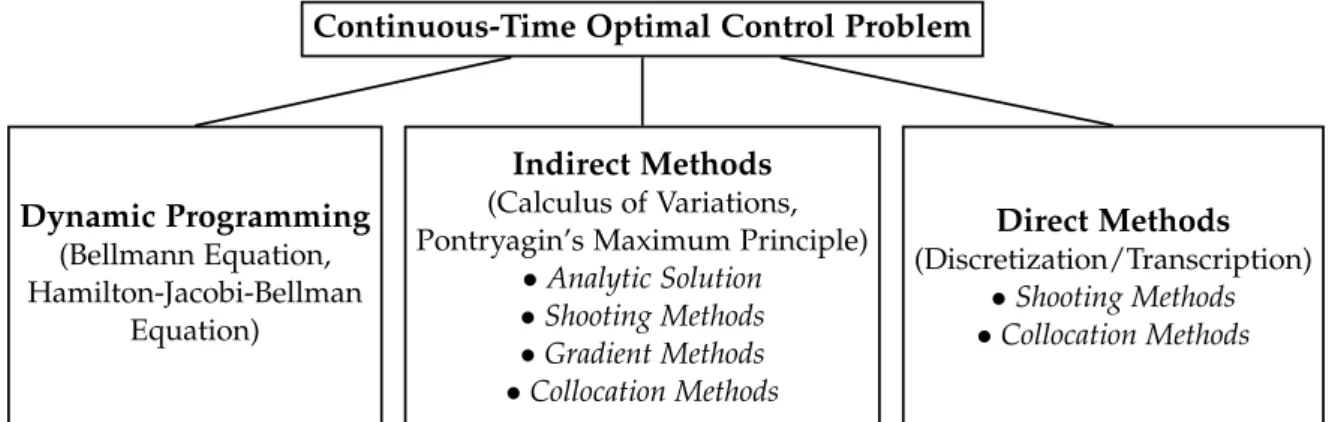
2.1. Optimal Control Methods . . . . 6 2.2. Model Predictive Control . . . 12 2.3. Time-Optimal Model Predictive Control . . . 14

3. Fundamentals 16

3.1. Dynamic System . . . 16 3.2. Feedback Control . . . 17 3.3. Benchmark Systems . . . 22

4. Global Uniform Grid for Time-Optimal Control 27

4.1. Direct Transcription Methods . . . 27 4.2. Solution to the Nonlinear Program . . . 33 4.3. Examples . . . 35

5. Time-Optimal Model Predictive Control 38

5.1. Shrinking-Horizon Closed-Loop Control . . . 38 5.2. Grid Size Adaptation . . . 44 5.3. Smooth Stabilizing Control . . . 47 6. Local Uniform and Quasi-Uniform Grid Representations 52 6.1. Uniformity Enforcement by Equality Constraints . . . 52 6.2. Approximation to the Uniform Grid . . . 53 6.3. Closed-Loop Control and Grid Adaptation . . . 56

7. Sparsity Structure Exploitation with Hypergraphs 59

7.1. Hypergraph Representation for Nonlinear Programs . . . 60 7.2. Sparse Derivative Computations . . . 62 7.3. Application to Time-Optimal Model Predictive Control . . . 66

8. Comparative Analysis and Benchmark Results 71

8.1. Time-Optimal Control with Variable Discretization Grids . . . 71

8.2. Comparison with Fixed Grid Methods . . . 78

8.3. Closed-Loop Control Performance . . . 81

9. Non-Uniform Grid for Bang-Singular-Bang Systems 84

9.1. Multiple Shooting Formulation . . . 84

9.2. Adaptation of Control Interventions . . . 90

9.3. Performance Comparison and Benchmark Results . . . 93

10. Conclusion and Outlook 97 A. Mathematical Definitions 101 A.1. Lipschitz Continuity . . . 101

A.2. Control Parameterization . . . 101

A.3. Numerical Solution to Initial Value Problems . . . 102

A.4. Fundamentals of Constrained Nonlinear Optimization . . . 103

B. Stability Definitions and Results 107 B.1. Lyapunov Functions for Stability . . . 107

B.2. Stability Results and Proofs . . . 108

C. Time-Optimal Control Methods – Extensions and Related Work 115 C.1. Related Methods from the Literature . . . 115

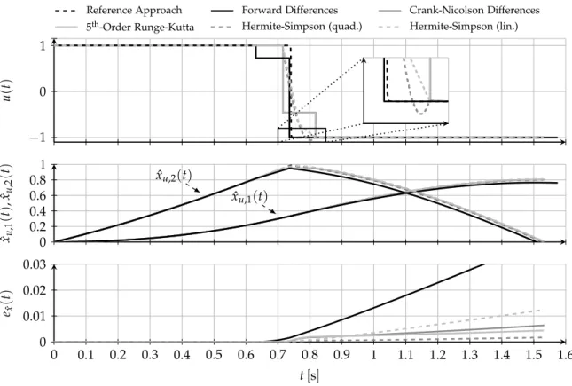
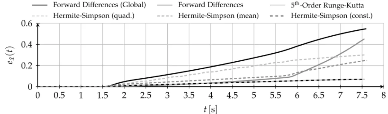
C.2. Types of Hermite-Simpson Collocation . . . 117

C.3. Minimum Number of Control Interventions . . . 120

C.4. Unconstrained Nonlinear Least-Squares Approximation . . . 121

D. Hypergraph for Nonlinear Model Predictive Control 129 D.1. Structural Sparsity Exploitation with Hypergraphs . . . 129

D.2. Comparative Analysis and Benchmark Results . . . 132

E. Implementation Details and Algorithms 136 E.1. Software Framework . . . 136

E.2. Optimization Algorithms . . . 137

F. Supplemental Results 142 F.1. ECP Industrial Plant Emulator Model 220 . . . 142

F.2. Benchmark Hardware and Results . . . 144

Bibliography 155

Nomenclature

General Symbols

ℓ 1 Absolute value norm

ℓ 2 Euclidean norm

T ¯ p Computation time required for solving the optimization problem T ¯ s Computation time required for preparing the optimization problem

∆t cpu Computation time for determining the control law

τ Auxiliary time parameter

θ Scalar weight for the ℓ ₁ -norm cost function θ ₀ Lower bound on θ to ensure time-optimality

ξ Auxiliary parameter in the Cauchy-Schwarz inequality Symbols and Functions for General Dynamic Systems and Control Tasks A System matrix of a linear system

B Input matrix of a linear system f ( · ) System dynamics vector field

f d ( · ) Sampled-data system dynamics vector field K Linear feedback gain matrix

L ¯ Lipschitz constant

¯

r Scalar parameter in the definition of Lipschitz continuity

p State dimension

φ ( · ) Solution to the initial value problem of the system dynamics

q Control dimension

¯ t Transformed time parameter (time transformation approach)

t f Final time

t s Initial time

t Time

u 1 ( t ) First component of control trajectory u ( t ) u 2 ( t ) Second component of control trajectory u ( t ) u ( t ) Control trajectory

u _f Final control respectively reference control u _dist ( t _µ ) Disturbance profile with closed-loop time t _µ u lin ( t ) Control trajectory of the linear system u max Upper bound on the control

u min Lower bound on the control

x 1 ( t ) First component of state trajectory x ( t ) x 2 ( t ) Second component of state trajectory x ( t ) x ( t ) State trajectory

x _f Final state respectively steady state

x _f,1 First component of the final state

x _f,2 Second component of the final state x _ref ( t ) Reference trajectory

x s Initial state

x _lin ( t ) State trajectory of the linear system x max Upper bound on the state

x min Lower bound on the state y ( t ) System output

y ₁ ( t ) First component of y ( t ) y 2 ( t ) Second component of y ( t )

Symbols and Functions for Predictions, Open-Loop Control and Direct Transcription β ₁ Coefficient for the linear term in the quadratic control polynomial β 2 Coefficient for the quadratic term in the quadratic control polynomial

∆t Global time interval t _{k +} 1 − ^t k , ∀ ^k

∆t _k Local time interval t _{k + 1} − ^t k

∆t _ϵ Threshold for inserting or removing intervals (grid adaptation)

∆t max Upper bound on the time interval

∆t min Lower bound on the time interval

∆t _ref Reference time interval for grid adaptation

∆t ^∗ Optimal global time interval t _{k + 1} − ^t k , ∀ ^k

∆t ^∗ _k Optimal local time interval t _{k + 1} − ^t k

t min Lower bound on the final time t f (hybrid cost approach) ι Running index for enhanced integration (non-uniform grid)

∆t _int Step size for the integration steps ∆t _k /N _int (non-uniform grid)

∆t _rem,k Remaining step width for interval ∆t _k (non-uniform grid)

∆u _k Control error at time instance t _k with respect to u f

∆x _k State error at time instance t _k with respect to x _f e x ˆ ( t _f ) Integral error at time t _f

e x ˆ ( t ) Integral error with respect to ˆ x _u ( t ) ( ℓ 2 -norm)

g ˜ ( · ) Integrand of the additional constraint equation (non-uniform grid) γ ₁ Coefficient for the linear term in the cubic state polynomial

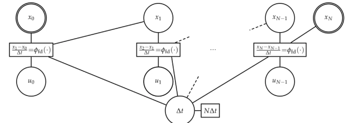
γ 2 Coefficient for the quadratic term in the cubic state polynomial γ 3 Coefficient for the cubic term in the cubic state polynomial h hs ( · ) State interpolant at t _{k + 0.5} in Hermite-Simpson collocation h _fd ( · ) Equality constraint for collocation via finite differences h _fe ( · ) Equality constraint for multiple shooting with forward Euler

I _adapt Number of iterations for grid adaptation

i General running index (multiple shooting grid, grid adaptation, fun- damentals of nonlinear optimization)

k ¯ Running index for accumulating time intervals of the local grid κ Running index for Levenberg-Marquardt and SQP iterations k Index for time instances (prediction)

ℓ( · ) Running cost

˜

m Number of controls in each shooting interval, ˜ m _i = m ˜ ∀ ⁱ

Nomenclature

˜

m _i Number of controls in the i-th shooting interval M Number of shooting intervals

N init Initial grid size N for grid adaptation N max Upper bound on the grid size N N min Lower bound on the grid size N

N Discretization grid size or horizon length

N ^∗ Minimum grid size respectively dead-beat horizon length N _crit Smallest grid size for which the non-uniform grid is feasible

k ¯ ₁ , ¯ k 2 , . . . , ¯ k 6 Auxiliary parameters in the explicit 5 ^th -order Runge-Kutta method N _b Number of control interventions (non-uniform grid)

N ˜ b Surplus in the number of control interventions (non-uniform grid) u _ϵ Similarity threshold for two consecutive controls (non-uniform grid) N int Number of integration steps for interval ∆t _k , ∀ ^k (non-uniform grid) N _int,k Number of integration steps for interval ∆t _k (non-uniform grid) ϕ _fd ( · ) Finite difference kernel function

ϕ _hs ( · ) Simpson quadrature of f ( · ) in Hermite-Simpson collocation

ϖ Running index for interstitial grid points k in each shooting interval Q ˜ Weighting matrix for the state error (Riemann sum approximation) Q State error weighting matrix in quadratic form cost

R ˜ Weighting matrix for the control effort (Riemann sum approximation) R Control effort weighting matrix in quadratic form cost

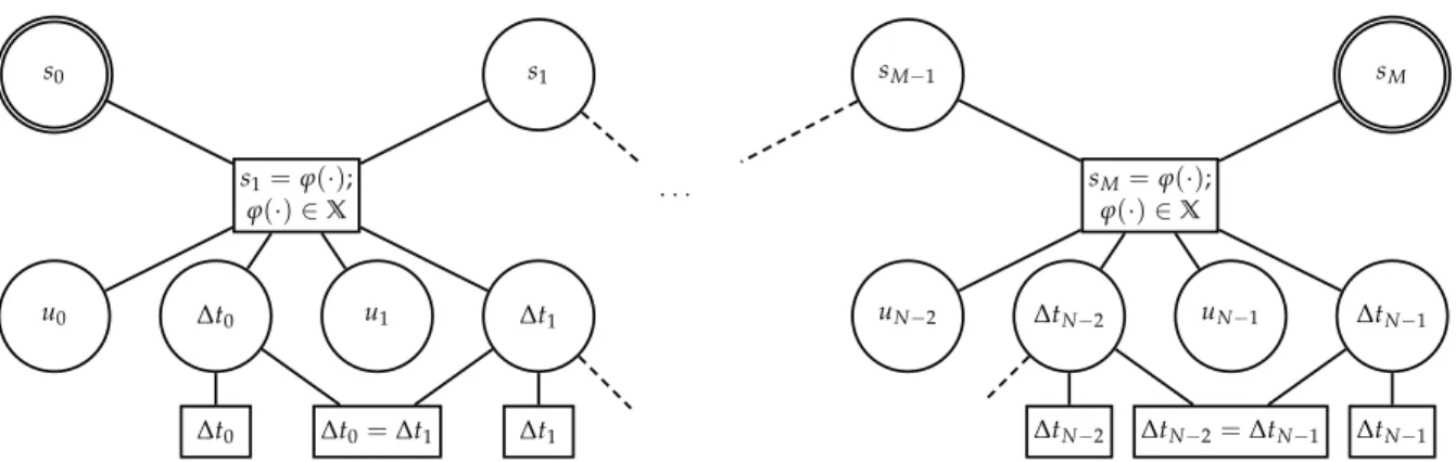
ρ Weight for the regularization term (non-uniform grid) s ¯ _k Slack variable with index k in the ℓ 1 -norm approach s _i Shooting node at time instance ˜ t _i , x _u ( t ^˜ _i ) : = s _i

˜ t _i Time instance with index i (multiple shooting grid) t 0 Initial time (prediction)

t _k Time instance with index k (prediction)

˜

u _i ( t ) Control trajectory on shooting interval [ t ^˜ _i , ˜ t _{i + 1} ] , u ( t + t ^˜ _i ) : = u ˜ _i ( t ) u ^∗ ( t; t _µ ) Optimal control trajectory at closed-loop time t _µ

u ^∗ ( t ) Optimal control trajectory

u ^∗ _k Optimal control at time instance t _k (prediction) u _k Control at time instance t _k , u ( t _k ) : = u _k (prediction)

V _dyn,N Cost for the non-uniform grid control problem with size N

V _dyn,N ^∗ Optimal cost for the non-uniform grid control problem with size N V _f ( · ) Terminal cost

V _k ( · ) Integral of the running cost on interval [ t _k , t _{k + 1} ] x _u,1 ( t ) First component of state trajectory x _u ( t ) (prediction) x _u,2 ( t ) Second component of state trajectory x _u ( t ) (prediction)

ˆ

x _u,1 ( t ) First component of state trajectory ˆ x _u ( t ) ˆ

x _u,2 ( t ) Second component of state trajectory ˆ x _u ( t ) ˆ

x _u ( t ) Open-loop state trajectory (for error calculation) x _u ( t ) State trajectory (prediction)

x _k State at time instance t _k , x _u ( t _k ) : = x _k (prediction) 1 _p Vector of ones with dimension p × ¹

I _n Identity matrix with dimension n × ⁿ

Symbols and Functions for Closed-Loop Control

∆t _µ,n Time interval between time instances t _µ,n and t _µ,n + 1

g f ( · ) Closed-loop system dynamics vector field µ ( · ) Control law

µ ₁ ( · ) First component of the control-law µ ( · ) µ 2 ( · ) Second component of the control-law µ ( · ) µ _dual ( · ) Dual-mode control-law

µ _lin ( · ) Control law of the local controller (dual-mode) n Index for time instances (closed-loop)

φ _µ ( · ) Solution to the initial value problem of g _f ( · ) t µ Time variable (closed-loop)

t _µ,n Time instance with index n (closed-loop) x _µ,1 ( t _µ ) First component of state trajectory x _µ ( t ) x µ,2 ( t _µ ) Second component of state trajectory x _µ ( t ) x µ ( t µ ) State trajectory (closed-loop)

Symbols and Functions for the Stability Analysis α 1 ( · ) Comparison function, α 1 ∈ K ∞

α ₂ ( · ) Comparison function, α ₂ ∈ ^K ∞

α _V ( · ) Comparison function, α _V ∈ ^K β ( · ) Comparison function, β ∈ ^KL η Distance from x _f (stability analysis)

Symbols and Functions for Nonlinear Programs and the Hypergraph

χ ( · ) Weighted quadratic penalty function for inequality constraints d ˜ Constant term in least-squares derivation

D (︁

Φ ( · ) , ∆z )︁

Directional derivative of Φ ( · ) with respect to ∆z.

∆z Parameter update vector

∆z ^∗ Optimal parameter update vector

e ^g _r Edge in the hypergraph that is associated with g _r ( · ) e ^h _s Edge in the hypergraph that is associated with h _s ( · ) e _l ^J Edge in the hypergraph that is associated with J _l ( · ) η _LS Growth rate for the least-squares approximation λ LM Levenberg-Marquardt damping factor

η _sqp Line-search parameter in sequential quadratic programming F ( z ) Least-squares cost vector with respect to parameter z

˜

g ( · ) Quadratic penalty function for inequality constraints g ( · ) General inequality constraint function

g _r ( · ) Component with index r in g ( · )

H Hessian of the least-squares problem and Hessian in the SQP h ( · ) General equality constraint function

h _s ( · ) Component with index s in h ( · )

I LM Number of Levenberg-Marquardt solver iterations I SQP Number of SQP solver iterations

J ( · ) General cost function

J _l ( · ) Cost summand with index l in J ( · )

Nomenclature

δ D Pertubation of finite difference calculations (first-order) δ H Pertubation of finite difference calculations (second-order) L ( · ) Lagrangian of a nonlinear program

L Number of summands in J ( · )

l Running index for summands in J ( · )

λ Lagrange multiplier for the equality constraint

λ ^∗ Optimal lagrange multiplier for the equality constraint λ ^∗ _i Optimal lagrange multiplier for the i-th equality constraint λ _i Lagrange multiplier for the i-th equality constraint

µ Lagrange multiplier for the inequality constraint

µ ^∗ Optimal lagrange multiplier for the inequality constraint µ ^∗ _i Optimal lagrange multiplier for the i-th inequality constraint µ m Penalty parameter in merit function Φ ( · )

µ _i Lagrange multiplier for the i-th inequality constraint

Φ ( · ) Merit function for line-search in sequential quadratic programming

˜

p Linear term in least-squares derivation

ψ ( · ) Weighted quadratic penalty function for equality constraints R Dimension of inequality constraint function g ( · )

r Running index for components of g ( · )

S Dimension of equality constraint function g ( · ) s Running index for components of h ( · )

σ 1 Penalty weighting parameter for equality constraints

˜

σ ₁ Square root of σ ₁

σ ₂ Penalty weighting parameter for inequality constraints

˜

σ 2 Square root of σ 2

τ sqp Line-search parameter in sequential quadratic programming Υ ˜ Number of unfixed vertices in the hypergraph

Υ Number of nominal optimization parameters

v _υ Vertex in the hypergraph that correspond to parameter z _υ

w Vector in constraint qualification conditions and second-order opti- mality conditions

˜

z υ ˜ Nominal optimization parameter with index ˜ υ z _υ Nominal optimization parameter with index υ

n _z Dimension of z

z Nominal (single) optimization parameter z ^∗ Optimal (single) optimization parameter

z max Upper bound on nominal optimization parameter z min Lower bound on nominal optimization parameter z ref,ω Fixed vector asigned to z ω for some 0 ≤ ^ω ≤ ^Υ z _ω Parameters with trivial assignments (see z _ref,ω ) Symbols and Functions for Benchmark Systems

a vdp Damping coefficient of the Van der Pol oscillator c _drag Drag coefficient of the rocket system

c roc Mass rate of change coefficient of the rocket system

˜

c ₁ Friction coefficient (ECP Model 220)

˜

c 2 Friction coefficient (ECP Model 220)

c 1 Linear damping coefficient (ECP Model 220)

c ₂ Coefficient for nonlinear damping (ECP Model 220) c 3 Slope in the nonlinear damping term (ECP Model 220) F _inertial Inertial force of the rocket system

F drag Drag force of the rocket system F _thrust Thrust force of the rocket system J ecp Moment of inertia (ECP Model 220) k ˜ 1 Motor specific constant (ECP Model 220) k ˜ 2 Motor specific constant (ECP Model 220) k ₁ Gain of the first motor input (ECP Model 220) k 2 Gain of the second motor input (ECP Model 220) m r ( t ) Mass of the rocket system at time t

m r,f Final mass of the rocket system

s r ( t ) Position of the rocket system at time t s _r,f Final position of the rocket system v r ( t ) Velocity of the rocket system at time t v r,f Final velocity of the rocket system Sets

B η ( x _f ) Ball around x _f with distance η C ( · ) Critical cone

∅ Empty set

E Set of edges in the hypergraph E e Set of indices of equality constraints F ( z ) Linearized feasible directions at z G ( V ^, E ) Hypergraph

A I ( z ) Set of indices of active inequality constraints with respect to z I Set of indices of inequality constraints

I Open time interval, I ⊂ ^R

K Set of indices that relate to redundant controls (non-uniform grid) N Neighborhood of an optimal parameter z ^∗

N Positive natural numbers excluding zero N ₀ Natural numbers including zero

Ω Feasible set for the nominal nonlinear program P global Set of optimization parameters for the global grid P local Set of optimization parameters for the local grid

P local,N Set of optimization parameters for the local grid with size N P Generic set for practical asymptotic stability

P _c ( · ) Controllability region with respect to U ^N P _{∆t min} ( x _f ) Controllability region to x _f up to time ∆t min

R ⁺ Positive real numbers excluding zero R ⁺ ₀ Positive real numbers including zero

S i Set of grid indices k in the shooting interval [ t ^˜ _i , ˜ t _{i + 1} ]

Nomenclature

S Lyapunov function state space, S ⊂ X T _Ω ( z ) Tangent cone at z

U Restricted control space, U ⊂ U U Control space, X ^: = R ^q

V Set of vertices in the hypergraph X _feas Feasible set in the TOMPC approach X Restricted state space, X ⊆ X

X _lin Forward invariant region of the local controller (dual-mode) X _f Terminal set, X _f ⊆ ^X

X State space, X ^: = ^{R p}

Y Generic forward invariant set

Z ˜ Set of nominal optimization parameters whose vertex is not fixed Z Set of nominal optimization parameters z _υ

Z r ^g Set of optimization parameters that directly affect g _r Z s ^h Set of optimization parameters that directly affect h _s Z _l ^J Set of optimization parameters that directly affect J _l Function Spaces

K Comparison functions (stability analysis) K ∞ Comparison functions (stability analysis) KL Comparison functions for (stability analysis) L Comparison functions (stability analysis)

L ^∞ ([ t 0 , t f ] , U ) Lebesgue integrable control functions on interval [ t 0 , t f ] L ^∞ ( R, U ) Lebesgue integrable control functions on R

U _k Control space on grid interval [ t _k , t _{k + 1} ]

U ^N ( t _f ) Control space of N piecewise polynomials up to time t _f Special Operators

⌈·⌉ Ceiling operator

| ^Z | Cardinality of set Z (only for sets)

| ^z | Absolute value of scalar z

⌊·⌋ Flooring operator

D _z f ( z 0 , · ) Jacobian of vector field f ( z, · ) with respect to z and evaluated at ( z 0 , · ) D f ( z 0 ) Jacobian of vector field f ( z ) with respect to z and evaluated at z 0

∥·∥ Arbitrary norm

∥·∥ 1 ℓ ₁ -norm (absolute value norm)

∥·∥ ² ℓ 2 -norm (Euclidean norm)

∥·∥ Q Weighted ℓ 2 -norm, for example ∥ ^z ∥ Q = √ z ^⊺ Qz max ( z 0 , z 1 ) Componentwise maximum of vectors z 0 and z 1

min ( z 0 , z 1 ) Componentwise minimum of vectors z 0 and z 1

∇ z J ( z 0 , · ) Gradient of scalar function J ( z, · ) with respect to z and evaluated at ( z 0 , · )

∇ ^J ( z ) Gradient of scalar function J ( z ) with respect to z and evaluated at z 0

∇ zz ² J ( z 0 , · ) Hessian of scalar function J ( z, · ) with respect to z and evaluated at ( z 0 , · )

∇ ^{2 J} ( z 0 ) Hessian of scalar function J ( z ) with respect to z and evaluated at z 0

Abbreviations and Acronyms

AD Automatic Differentiation

BFGS Broyden-Fletcher-Goldfarb-Shanno algorithm IPOPT Interior Point Optimizer

KKT Karush-Kuhn-Tucker

LICQ Linear Independence Constraint Qualification LQR Linear Quadratic Regulator

MFCQ Mangasarian-Fromovitz Constraint Qualification MPC Model Predictive Control

NRMSE Normalized Root Mean Square Error

nz non-zeros

OSQP Operator Splitting Quadratic Program PID Proportional-Integral-Differential RTI Real-Time Iteration Scheme

SQP Sequential Quadratic Programming

w.r.t. with respect to

1

Introduction

1.1. Motivation

In a number of industries, minimizing time is essential to increasing the productivity of automation solutions. To give a few examples, gantry cranes lift and transport a large number of containers in ports to meet the increasing demand for import and export goods. In addition to sophisticated logistics, faster crane control is crucial to increase productivity. In the field of warehouse robotics, mobile robots are also ex- pected to navigate as fast as possible while avoiding obstacles. The productivity in the area of automated assembly at automobile manufacturers correlates strongly with the execution speed of their robotic manipulators. Racing is also dedicated to minimizing lap times as a central objective. In most of today’s industrial applications, however, linear control concepts such as PID or robust H _∞ -control [Zho+96] as well as linear quadratic regulators (LQR) [KS72] are used due to their simple realization and im- plementation. The minimization of time is only achieved by an aggressive tuning of the control parameters. These conventional controllers cannot explicitly incorporate constraints on control respectively state variables such as limited crane swing, obsta- cle avoidance or bounded robot respectively car velocities without conservatism and further restrictions [Sch+97]. Practical control systems are therefore not operated at

Time t µ

Current time t 0 t 1 Final time t _f

Prediction (horizon)

Control bound u max

Final state x f

Past

input sequence u ^∗ ₀ Predicted

input sequence Past

trajectory

Predicted trajectory Current state x u ( t 0 )

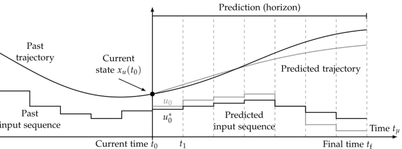
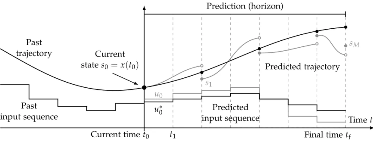
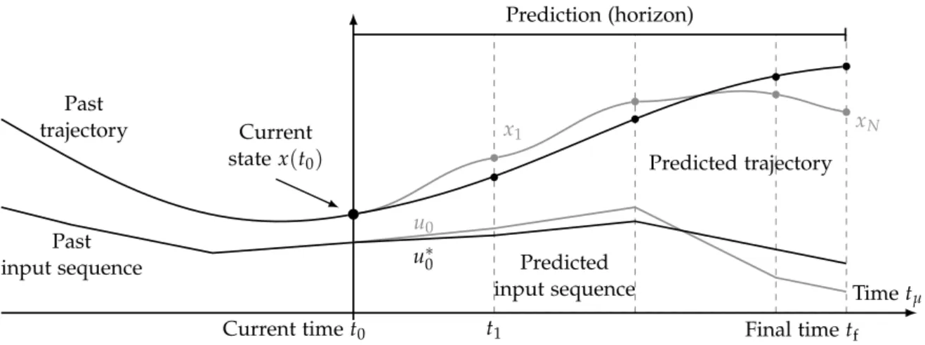
Figure 1.1.: Receding horizon principle in MPC.

Model Predictive Controller

Plant

Observer Control law

µ ( t µ ) : = u ^∗ ₀

Output y ( t µ )

Current state x u ( t 0 ) : = x µ ( t µ ) Final state

x f

x

tf Prediction (horizon)

x

( t

)

tµ

t0 t1 tf

Prediction (horizon)

x

( t

) _u

max

x

u0

t

t0 t1 tf

Prediction (horizon)

x

( t

) _u

max

x

u^∗₀

Optimization

Figure 1.2.: Typical point-to-point MPC architecture. Subscript µ indicates the context to the closed-loop evolution wheres subscript u refers to the prediction.

their potential performance limits in order to achieve actual time-optimality.

In recent decades, model predictive control (MPC) became an established and compre- hensive framework for controlling nonlinear systems under appropriate performance criteria and explicit adherence to constraints. In each sampling interval, the model predictive controller employs a (nonlinear) model of the dynamic system to predict and optimize the future evolution of the system within a specified temporal horizon as illustrated in Figure 1.1. The first portion of the optimized control sequence is com- manded to the plant before the optimization process is repeated. Consequently, the closed-loop architecture as depicted in figure 1.2 consists of the following primary ingredients:

• Knowledge of the full state of the plant which is either directly measurable or estimated by a state observer

• Numerical simulation of the system trajectories based on an internal model

• Constrained optimization algorithm

Even if the basic design of a model predictive controller is rather intuitive due to

the simple definition of performance criteria and constraints in comparison to, for

example, a PID controller, it’s nowadays application in practice is still limited to slow

processes [PH14]. Especially the underlying numerical simulations and (iterative) con-

strained optimization are usually difficult to solve for generic nonlinear respectively

nonconvex problem formulations. Also, its online realization is computationally in-

tensive. Once these problems are adequately solved, MPC has the potential to replace

PID, H _∞ and LQR controllers in industrial applications to maximize performance while

maintaining increasing system complexity. To this end, recent researches focus on

developing numerically efficient MPC realizations to enable their utilization also for

faster systems such as mechatronic systems. However, these realizations mainly con-

sider MPC with quadratic cost terms, in particular, the minimization of the state error

1.2. Contribution and Outline

and control effort, which limits its application to areas that require true time-optimal- ity. The already excellent and predictable potential of MPC motivates the dedicated expansion to realize time-optimal control tasks in future industrial applications.

1.2. Contribution and Outline

This thesis contributes to the following two central research questions:

1. How to design time-optimal controllers for nonlinear systems under the explicit consideration of constraints, particularly in the framework of MPC?

2. How to realize time-optimal MPC in a computationally efficient way?

The first research question is addressed by introducing direct transcription meth- ods that first discretize and then optimize the subordinate optimal control problems.

In contrast to conventional methods, the underlying discretization grid is explicitly treated as temporally variable during optimization. This principle procedure makes it possible to replace the entire transition time by local time information which is defined only between two successive discrete states. Accordingly, minimizing the local time information leads to the overall minimum transition time. The resulting optimal con- trol problems retain their inherent sparse structure, even if time is explicitly regarded as an optimization parameter. Many iterative optimization algorithms already take sparse algebra into account, but the calculation of first- and second-order derivatives in each optimization step is still very demanding. A hypergraph representation of the optimal control problems inherently captures their sparse structure and enables efficient structure-depending finite difference computations. The hypergraph recon- figures itself online with little computational effort, especially for different problem dimensions, which later proves to be decisive for the proposed time-optimal control approaches.

The following list provides a brief overview of the chapters contained in this thesis including their central contribution:

Chapter 2: This chapter summarizes the current state of the art of time-optimal MPC and related work done in the context of optimal control as well as MPC in general. A particular focus lies on optimal control methods with free final time and variable switching points from optimal (feedforward) control.

Chapter 3: Preliminaries and key definitions which are necessary for the following

chapters are summarized. In addition to the classification of different con-

trol tasks for time-optimal control, the mathematical foundation for sampled

closed-loop systems is provided. Also, the general continuous-time time-optimal

control problem is defined which serves as an essential basis for all direct tran-

scription methods presented in the following chapters. The chapter also presents

two benchmark systems and a real experimental system which are referred to in

numerous examples throughout the thesis.

Chapter 4: This chapter presents a global uniform discretization grid with a single temporal optimization parameter. Several direct transcription methods are defined, in particular multiple shooting, Hermite-Simpson collocation and collocation based on finite differences. This chapter also highlights some effects that can occur when collocation with higher-order control representations is imposed.

Chapter 5: The previously defined global uniform discretization grid is now integrated with state feedback. First, various challenges and issues for its direct closed-loop application are discussed. Then, a shrinking horizon grid adaptation scheme is presented for which (practical) asymptotic stability results are derived under reasonable assumptions. The grid adaptation strategy is further extended to maintain a desired temporal resolution. As known from general time-optimal control, the control sequence is affected by chattering while stabilizing the system at the steady state. To remedy this, the controller based on variable discretization grids is either embedded in a dual-mode formulation or supplemented by a quadratic form cost function to achieve smooth stabilization.

Chapter 6: This chapter introduces two further variable grid representations based on multiple temporal optimization parameters. The first approach enforces uniformity by additional equality constraints. Even though the solution is identical to the global uniform grid, its underlying sparsity structure is different as it is pointed out later in Chapter 7. The second approach omits additional uniformity constraints and tries to achieve a quasi-uniform grid in terms of a least-squares cost function.

Furthermore, the chapter provides several examples and remarks regarding grid adaptation and closed-loop integration.

Chapter 7: This chapter presents the hypergraph representation to exploit sparsity for derivative computations as mentioned above. Originally, the hypergraph is borrowed from the context of robotics and this chapter extends it to nonlinear programs arising in MPC. The applicability is not limited to time-optimal control problems. The procedure seamlessly extends to general optimal control and MPC problems.

Chapter 8: This chapter provides extensive benchmark results and a comparative anal- ysis of the previously defined variable grid approaches. Furthermore, the con- cepts are compared to related and recent methods in the literature for both the open-loop and the closed-loop performance.

Chapter 9: Based on a modified multiple shooting approach, this chapter proposes a non-uniform grid which is well suited for control systems that exhibit the bang-singular-bang property. Practical stability results are provided under milder conditions than for the uniform grid. Furthermore, a proposed grid adaptation scheme seeks for the ideal number of switching points online.

Chapter 10: This chapter summarizes the central results, provides concluding remarks

for the developed concepts and suggests possible directions for future works.

1.2. Contribution and Outline

In addition, the appendix contains extensions to the proposed approaches and further supplementary material.

The following list summarizes the most important contributions and highlights of this thesis:

1. Time-optimal control via direct transcription and variable discretization grids:

• Global uniform grid,

• Local uniform grid,

• Quasi-uniform grid,

• Non-uniform grid for bang-singular-bang control.

2. Analysis and comparison of several numerical schemes to approximate the sys- tem dynamics in terms of time-optimal control

• Multiple shooting,

• Collocation via finite differences,

• Collocation via quadrature (Hermite-Simpson).

3. Feedback control:

• Theoretical results on stability and recursive feasibility,

• Practically motivated extensions and realizations.

4. Structural sparsity exploitation and online optimization:

• Hypergraph formulation for sparse derivative computations,

• C++ software framework for fast MPC and direct optimal control,

• Specialized sequential quadratic programming algorithm.

2

Related Work

Model predictive controllers solve an optimal control problem at each sampling inter- val. Consequently, their development, application, and success are closely related to advances and achievements in the field of optimal control and optimization in general.

In particular, numerical approaches are preferred as they are suitable for more generic and complex applications. This chapter gives a brief overview of the current state of the art in time-optimal MPC and the most important areas that are decisive for its de- velopment. These include feedforward optimal control, optimal control with free final time, model predictive control (especially in the context of continuous-time, nonlinear systems and real-time optimization).

2.1. Optimal Control Methods

The main objective of optimal control is to find a control policy that operates or controls a system under certain optimality criteria and constraints. While for certain problem formulations analytic solutions exist to form a closed-loop control law, the more general goal is to find an open-loop control policy (numerically). The following overview mainly focuses on continuous-time optimal control formulations as they form the basis for methods presented in this thesis. Continuous-time optimal control problems are expressed in terms of cost and constraint functionals. Their solution is a control trajectory and thus a function of time. Methods for solving such problems are categorized into three main types: dynamic programming, indirect and direct methods (refer to Figure 2.1). For analytic solutions, especially for the important class of unconstrained infinite-horizon optimal control of linear systems with quadratic form cost functions, commonly known as Linear Quadratic Regulator (LQR), the reader is referred to [Kal60; Wil71].

2.1.1. Dynamic Programming

Dynamic programming is based on the principle of optimality developed by Bellmann

[Bel57]. The principle states that “an optimal policy has the property that whatever

the initial state and initial decisions are, the remaining decisions must constitute an

optimal policy with regard to the state resulting from the first decisions” [Bel54].

2.1. Optimal Control Methods

Continuous-Time Optimal Control Problem

Indirect Methods (Calculus of Variations, Pontryagin’s Maximum Principle)

• Analytic Solution

• Shooting Methods

• Gradient Methods

• Collocation Methods Dynamic Programming

(Bellmann Equation, Hamilton-Jacobi-Bellman

Equation)

Direct Methods (Discretization/Transcription)

• Shooting Methods

• Collocation Methods

Figure 2.1.: Overview of different methods to solve continuous-time optimal control problems.

Consequently, the optimal control problem is divided into several subproblems. For discrete-time systems this fact is mathematically formulated by the Bellmann equation.

In the case of continuous-time systems, a partial differential equation which is referred to as Hamilton-Jacobi-Bellmann equation has to be solved. A collection of established dynamic programming methods is summarized in [Ber95]. Dynamic programming methods usually require the sampling of the entire time, state and control space which guarantees to find the globally optimal solution, but on the other hand makes them intractable for larger system dimensions. This is often referred to as curse of dimen- sionality [Pow11]. Approximate dynamic programming methods try to relax the curse of dimensionality [Pow11]. This can be achieved, for example, by applying function approximations to reduce the grid size [Grü97], or by iteratively examining samples in the grid close to the actual solution [Luu10].

2.1.2. Indirect Methods

Indirect methods transform the continuous-time optimal control problem into a set of ordinary differential equations and boundary conditions using calculus of varia- tions. The solution is then obtained by solving the resulting boundary value prob- lem (first-order necessary conditions), which consists of state and adjoint variables.

Pontryagin’s maximum principle extends the necessary condition for optimal con- trol problems with constraints [Pon87]. Numerically, the boundary value problem is solved with shooting or collocation methods, similar to the direct methods. There- fore indirect methods are often referred to as first optimize and then discretize methods.

However, they solve simultaneously for the continuous state and adjoint variables. The latter complicates its initialization with a meaningful initial guess, since an intuitive physical interpretation is missing. In addition, the domain of convergence is usually smaller compared to dynamic programming and direct methods [Bet98]. On the other hand, indirect methods are still frequently used due to their high accuracy and fast convergence close to the optimal solution compared to direct methods [Pas12].

2.1.3. Direct Methods

Direct methods respectively direct optimal control or direct transcription methods

first discretize the original problem representation and then optimize the resulting ap-

Time t µ

Current time t 0 t 1 Final time t _f

Prediction (horizon)

Current state x u ( t 0 ) Past

trajectory

Past input sequence

Predicted trajectory

u 0

u ^∗ ₀ Predicted

input sequence

Figure 2.2.: Illustration of the single shooting method: Example initialization (gray) and con- verged solution (black). The first control is denoted by u ₀ and u ^∗ ₀ its optimal value.

proximation. By discretization of the continuous-time optimal control problem it is transformed into a (non-)linear program, which is subject to a finite set of optimiza- tion parameters, especially states and controls at discrete timestamps. Consequently, cost and constraint functionals are replaced by ordinary functions. A wide range of established constrained optimization algorithms exists to solve nonlinear programs numerically [NW06].

Direct methods are further categorized into sequential and simultaneous approaches.

A well known sequential method for continuous-time problems is single shooting.

Single shooting defines the control trajectory in terms of piecewise constant controls subject to optimization. The corresponding state trajectory is then obtained by solving the initial value problem numerically with respect to a given initial state, all controls and the system dynamics equations [Bet98]. Consequently, an iterative optimization algorithm simulates the entire state trajectory at least once in each iteration to evaluate cost functions and constraints before computing a new update of the control sequence.

This procedure is repeated until convergence (refer to Figure 2.2). The major drawback of this approach is its limited numerical stability and usually low convergence. The intermediate results of the optimization are very sensitive to changes at the beginning of the control sequence that cause significant nonlinear changes at the end [Bet98].

On the other hand, simultaneous approaches discretize and optimize both states and controls. For example, multiple shooting discretizes the state trajectory on the same or coarser grid than the controls [BP84]. These introduced state variables are explicitly considered as optimization parameters called shooting nodes and the resulting grid partitions are called shooting intervals (refer to Figure 2.3). Optimization algorithms solve an isolated initial value problem for each shooting interval with the shooting node as the starting point. The nonlinear program is extended by additional deflection constraints that enforce connectivity among shooting intervals. Although the number of optimization parameters to be determined is larger than for single shooting, con- vergence is usually faster [Bet98]. Furthermore, the optimization problem has a sparse structure which is exploited in [Lei+03].

Direct collocation constitutes another well established simultaneous approach which

2.1. Optimal Control Methods

Time t µ

Current time t 0 t 1 Final time t _f

Prediction (horizon)

Current state s 0 = x ( t 0 ) Past

trajectory

Past input sequence

s M

Predicted trajectory s 1

u 0

u ^∗ ₀ Predicted

input sequence

Figure 2.3.: Illustration of the multiple shooting method: Example initialization (gray) and converged solution (black). Shooting nodes are denoted as s ₀ , s ₁ , . . . , s _M .

discretizes both the state and control trajectory. The basic idea is to approximate the system dynamics and cost functions using a predefined set of basis respectively kernel functions. The system dynamics equations are fulfilled at the discrete time instants, which is enforced by adding a set of algebraic equality constraints to the nonlinear program [Tsa+75]. Established candidates for basis functions are finite difference ap- proximations and quadrature rules, which usually lead to piecewise linear, quadratic or cubic polynomials (splines) for the states and control trajectory [Str93; Kel17]. An example with a cubic Hermite spline as state and piecewise linear spline as control trajectory is shown in Figure 2.4. Direct collocation usually requires a larger num- ber of optimization parameters in comparison to multiple shooting. Note, numerical integration with step size control can be easily integrated in multiple shooting, but collocation requires to adapt the whole temporal grid or the basis functions itself to achieve higher accuracies [Sag06]. However, whereas multiple shooting is usually pre- ferred for optimal control problems with relatively simple controls, collocation meth- ods achieve higher accuracies for tasks in which more complex control trajectories are necessary. For the sake of completeness, two specializations of direct collocation have become established in recent decades: Orthogonal collocation in which basis functions vary along the temporal grid (for instance polynomials of different orders) [Bie84];

and pseudospectral optimal control methods which define a single but higher-order polynomial for the complete grid. Pseudospectral methods converge with a spectral (exponential) rate which is faster than any polynomial rate [Hes+07; RK12].

2.1.4. Free Final Time, Switching Points and Time-Optimal Control

The majority of optimal control problems are solved according to a fixed temporal grid such that only controls and states are optimized. On the other hand, there are many applications in which the temporal grid or the final time must also be optimized.

For example, the time required for guiding a system to another state is unknown in advance or the optimal control problem could be infeasible for the specified final time.

The switching points of the control sequence (which coincide with the grid points)

Time t µ

Current time t 0 t 1 Final time t _f

Prediction (horizon)

Current state x ( t 0 ) Past

trajectory

Past input sequence

x _N Predicted trajectory x 1

u 0

u ₀ ^∗ Predicted input sequence

Figure 2.4.: Illustration of a collocation method: Initialization (gray) and converged solution (black). A cubic spline is selected for the state trajectory and a linear spline for the control.

States at grid points are denoted by x ₀ , x ₁ , . . . , x _N .

also do not correspond to those of admissible solutions.

In time-optimal control, the total transition time respectively the final time itself is subject to optimization compulsively. Many plants are controlled either at control or state limits. Thus many practical time-optimal control problems consist of either bang-bang, bang-singular-bang or a small finite set of piecewise constant controls.

With such problems, the number of effective switching points is often significantly smaller than the ordinary temporal resolution of the a priori defined discretization grid. Feldbaum’s well-known theorem states that the time-optimal control sequence of an unconstrained linear system with state dimension p and only real eigenvalues exhibits at most p switches [Pon87]. Sussmann provides conditions for nonlinear con- trol-affine systems with bounded controls such that the resulting time-optimal control is bang-bang [Sus79]. Furthermore, he proves that nonlinear two-dimensional systems with a single affine control are of bang-singular-bang type [Sus87b; Sus87a]. Even though proving the bang-singular-bang property for nonlinear systems is difficult or intractable in general, many practical applications and experiments reveal bang-sin- gular-bang control sequences.

A numerical method for time-optimal control of linear systems with constraints is presented in [Fat68] and [TK71]. The approach partitions the complete time interval t _f into N uniform subintervals of length t _f /N and represents the control trajectory as piecewise constant with respect to the subintervals. Also, constraints are imposed only at the grid points of the subintervals. The so-called set of attainability describes all initial states from which admissible control functions produce admissible trajectories.

With this convex set, an auxiliary linear program is defined which is solved for example using the simplex method [TK71].

In order to deal with the free final time and hence nonlinear time-optimal control

problems, a time-scaling respectively time transformation is presented and applied

in [QD73; Jen+91; Teo+91]. The control trajectory is parameterized as a sequence

of piecewise constant controls. An overview of different canonical forms of optimal

control problems including the time transformation approach is presented in [II02].

2.1. Optimal Control Methods

Maurer and Oberle provide second-order sufficient conditions for problems with a free final time based on the proposed time transformation [MO02]. Refer to Appendix C.1.1 for the mathematical formulation of the approach.

Teo et al. present an optimal control formulation in which the temporal grid and its individual grid partition lengths are also subject to optimization and hence includes variable switching points [Teo+91]. The authors propose two alternative parameteri- zations: Either the actual controls are kept constant and just the switching points are determined or both controls and the switching points are subject to optimization. The authors provide non-smooth gradients of the cost functionals and constraints which are derived based on the results in [Has76] and which depend on first-order neces- sary conditions (Hamiltonian). Due to the discontinuous gradients (required for the proposed gradient-based indirect method) and the discontinuity of the system dy- namics equations at the switching points, the approach was “never implemented for a practical problem” [Teo+99].

Later in [Teo+99] the so-called control parameterization enhancing transform for con- strained optimal control problems is presented. Hereby, the original grid and switching times are mapped on to a uniformly spaced grid in a new time scale similar to the previously mentioned time transformation approach but with individual scalar pa- rameters for the different grid partitions. The grid is now fixed with respect to the new time scale (usually every grid partition is of length 1) and the system dynamics equa- tion is transformed similarly. Hence standard numerical optimal control algorithms can be utilized. This method is applied to time-optimal control problems in [Lee+97]

which involves the transformation and minimizes the scalar time mapping function.

In [Lee+99] the control parameterization enhancing transform is applied to discrete- valued control problems and in [Li+06] to switched systems. Further applications are summarized in [Reh+99]. Related work in [Vos10] formulates a direct method for bang-bang control and provides first- and second-order conditions as well as first- and second-order variational derivatives of the state trajectory with respect to the switching times.

An approximate time-optimal solution to an optimal control problem tailored for flexible structures with linear dynamics is provided in [Alb02]. The approach utilizes an indirect method to solve the optimal control problem. The infinite time-derivative at the switching times is replaced by a finite magnitude. For single-input nonlinear systems, [Kay03] approximates the time-optimal control problem in the arc time space (duration of arcs). The authors propose a dedicated approach to seek feasible but not necessarily optimal switching points [KN96]. With an application to the lap-time minimization of race cars, an optimal control formulation with different dynamics models is presented in [KS10; KS12].

Kashiri et al. propose an iterative indirect method to solve time-optimal control prob-

lems [Kas+11]. As for indirect methods in general, the method heavily relies on a

proper initialization for which the authors develop a dedicated strategy.

2.2. Model Predictive Control

The development of MPC concepts began in the 1960s. State space models became popular for the controller design, in particular the LQR [Kal60; Wil71] and its extension by a Kalman filter for state estimation which is referred to as linear quadratic Gaussian regulator [Kal60; Ath71]. However, even if the solution is obtained analytically, the ap- proach is restricted to quadratic cost functions and is only applicable to unconstrained linear systems.

The receding horizon concept enables constrained real-time optimization during feed- back control. Lee and Markus formulate the fundamental concept of MPC:

“One technique for obtaining a feedback controller synthesis from knowledge of open-loop controllers is to measure the current control process state and then compute very rapidly for the open-loop control function. The first portion of this function is then used during a short time interval, after which a new measurement of the process state is made and a new open-loop control function is computed for this new measurement. The procedure is then repeated.” [LM67]

Early practical MPC realizations are defined in terms of impulse response models [Ric+67; Ric+77] and step response models (dynamic matrix control) [CR80; QB03].

Albeit not directly related to MPC but to predictive control in general, another early concept called internal model control requires a model of the plant dynamics during runtime in order to realize a pure feedforward control scheme in the absence of model mismatch and disturbances. In practice, an additional feedback part compensates for those errors [GM82; Mor83].

Since the late 1990s and early 2000s the majority of research in MPC considers state space models either in discrete time or as sampled-data systems. For an overview of influential contributions in MPC at that time, the reader is referred to [QB97; Hel+98;

MH99; QB03; MS04]. The fundamental stability results of MPC are summarized in [May+00; GP17; Raw+17]. Especially the quasi-infinite horizon scheme guarantees stability for nonlinear systems under certain conditions [CA98; FA03; HL02]. Stabil- ity results on considering variable final times generally in the context of MPC are provided in [MM93; May95].

To apply MPC to fast systems, such as mechatronic systems, the interest in efficient

numerical realizations has grown considerably in the last two decades. The majority of

recent approaches to continuous-time dynamics focus on direct methods that solve the

underlying optimal control problem using a nonlinear program with finite parameters

as described in Section 2.1.3. Diehl et al. propose multiple shooting to solve contin-

uous-time system dynamics in MPC [Die+02]. Multiple shooting usually achieves a

better convergence rate due to its sparse albeit larger problem structure. The real-time

iteration (RTI) scheme reduces the computational effort in each sampling instance by

merely applying a single warm-started sequential quadratic programming (SQP) step

at each sampling interval [Die+05; Gro+16]. Kouzoupis et al. combine the RTI scheme

with different first-order methods in order to analyze its application to embedded

nonlinear MPC [Kou+15a]. To handle stiff systems, implicit integrators are preferred

over explicit ones. Recently, lifted integrators based on the inexact Newton method

2.2. Model Predictive Control

reduce the overall computational cost [Qui+15a; Qui+15b]. Zanelli et al. modify the RTI scheme to significantly reduce the number of variables subject to optimization by applying a backward Riccati sweep to a subset of the horizon [Zan+17]. Other approaches are based on early-terminating interior point methods that also exploit the sparsity of the problem structure in order to allow an efficient computation [WB08;

WB10; Ric13; Pak+13]. Simultaneous methods and warm-starting techniques are key to efficiency. Warm-starting in the context of real-time optimization assumes that the (updated) solution of the previous sampling interval provides a proper and reasonable initialization for the optimization in the current step. Depending on the warm-start strategy, the initialization is improved a priori, for example, by shifting the temporal grid. For quadratic programming, the sparse structure of the nonlinear program is exploited by condensing techniques, for example in [Jer+11; Kou+15b; Fri+16]. An- other way to increase efficiency is to remove inactive and obsolete constraints online, as proposed for linear systems in [JM13; Jos+15; Jos+17].

An efficient method based on projected gradients is presented in [GK12] within a real-time capable MPC scheme. Regarding linear systems, the approach by Zeilinger et al. guarantees stability and feasibility under hard real-time conditions [Zei+14]. Tai- lored gradient methods are recently applied to systems governed by partial differential equations [Rhe+14]. Saturation functions transform the underlying optimal control problem into an unconstrained one. A two-stage transformation technique with in- terior penalties is applied to nonlinear MPC in [KG16] to solve an unconstrained auxiliary MPC problem using an efficient gradient method. Nielsen et al. focus on the parallelization of the Newton step arising in both active-set and interior-point solvers by exploiting the sparse structure of the nonlinear program as well [NA15].

Move-blocking MPC methods reduce the number of control actions while keeping the horizon lengths relatively large. Either of these methods keep the control constant beyond the so-called control horizon or multiple controls in between the horizon are kept constant [Cag+04; Cag+07; GI10]. Move-blocking with a single degree of freedom in control and a tailored optimization strategy is considered in [Mak+18b].

Most of the above methods have in common that they compute at least first-order and often second-order derivatives of the cost function respectively constraints. If closed-form analytic derivatives are not available, they are computed automatically in numeric form. Often, the numeric computation relies on finite differences, usually central differences, to achieve the desired precision. On the other hand, automatic differentiation (AD) recently emerged as a popular and ubiquitous approach for com- puting exact derivatives as in the ACADO toolkit [Hou+11b]. AD inherently retains the sparse structure of the optimal control problem and avoids the numerical evaluation of structured zero elements in first- and second-order derivatives. CasADi [And13]

constitutes a mature and efficient open-source AD framework frequently reported in the MPC literature as the preferred tool in the realm of optimal control. The framework of AD provides an elegant and simple way to formulate the optimal control problem by merely formulating the mathematical expressions of the nonlinear program while preserving its sparse structure.

Automatic code generation strategies became popular during the last years in order

to generate tailored and efficient C code [Vuk+13]. Code generation plays an impor-

tant role in order to realize MPC on embedded systems [Kuf+15]. The previously mentioned AD frameworks feature code generation capabilities.

Explicit MPC solves the general parameterized optimization problem offline. The optimal control action for the current state and target is extracted from a precom- puted lookup table. The explicit approach requires the a priori discretization of the operational space. A well-known bottleneck is that the memory requirements grow exponentially with the dimension of the state space, thus limiting the approach to low-order dynamics. Selected methods for linear systems are presented in [Kou+11;

MK11] and for nonlinear systems in [Joh04; Pin+13; Tri+16].

2.3. Time-Optimal Model Predictive Control

The previously mentioned MPC approaches mainly consider cost functionals that depend on the state and control trajectory, especially a quadratic form cost. Thus, grids for the discretization of continuous-time dynamics are usually fixed during runtime.

The literature mentions time-optimal MPC research rarely. Nevertheless, some contri- butions and applications rely on the basic time transformation as discussed in Sec- tion 2.1.4. Theoretical stability results for controllers considering the time transforma- tion are intractable and are hence not yet available in the literature (see also [Ver+17]).

Zhao et al. provide a time-optimal MPC scheme for the control of a spherical robot based on the time transformation [Zha+04]. A hybrid cost function that also con- siders quadratic form cost achieves stabilization. The transformed time is bounded from below close to the target state such that only the quadratic form cost becomes active. Verschueren et al. compute time-optimal motions along a Cartesian path for robotic manipulators [Ver+16b]. Time transformation is applied to the underlying time-optimal control problem to map states and controls onto a fixed integration grid.

A nonlinear MPC method for time-optimal point-to-point transitions which does not rely on time transformation is presented in [Van+11b; Van+11a]. The method called TOMPC for time-optimal MPC minimizes the settling time in a two-layer optimization routine. The settling time is defined in terms of the horizon length N. The outer loop incrementally reduces the horizon of the control sequence N until the inner loop nonlinear program with a standard quadratic form cost fails to generate a feasible solution for the allocated time horizon. Since the cost function minimizes the distance of discrete states to the final state, the solution with the shortest feasible horizon is quasi time-optimal. Due to the lower bound on the time horizon, the algorithm behaves like a conventional MPC in the vicinity of the final state and therefore guarantees stability. The computation time strongly depends on the initial estimate of the settling time, as it determines the number of iterations in the outer loop time horizon reduction.

Refer to Appendix C.1.2 for a mathematically more detailed description of TOMPC.

The work of [PP14] presents the analysis and design of time-optimal feedback control with variable horizon lengths N.

An alternative approach that follows a reference path in minimum time is presented in

[Lam12]. Time-optimality is nearly achieved in case of long time horizons. A time-op-