Theoretical analysis of diversity mechanisms for global exploration

TECHNISCHE UNIVERSIT ¨ AT DORTMUND REIHE COMPUTATIONAL INTELLIGENCE COLLABORATIVE RESEARCH CENTER 531

Design and Management of Complex Technical Processes and Systems by means of Computational Intelligence Methods

Theoretical Analysis of Diversity Mechanisms for Global Exploration

Tobias Friedrich, Pietro S. Oliveto, Dirk Sudholt, Carsten Witt

No. CI-237/08

Technical Report ISSN 1433-3325 January 2008

Secretary of the SFB 531 · Technische Universit¨ at Dortmund · Dept. of Computer Science/LS 2 · 44221 Dortmund · Germany

This work is a product of the Collaborative Research Center 531, “Computational

Intelligence,” at the Technische Universit¨ at Dortmund and was printed with financial

support of the Deutsche Forschungsgemeinschaft.

Theoretical Analysis of Diversity Mechanisms for Global Exploration

Tobias Friedrich

Algorithms and Complexity Group Max-Planck-Institut f¨ ur Informatik

Saarbr¨ ucken, Germany

Pietro S. Oliveto ¹

School of Computer Science University of Birmingham Birmingham, United Kingdom

Dirk Sudholt ²

Fakult¨ at f¨ ur Informatik, LS 2 Technische Universit¨ at Dortmund

Dortmund, Germany

Carsten Witt ²

Fakult¨ at f¨ ur Informatik, LS 2 Technische Universit¨ at Dortmund

Dortmund, Germany

Abstract

Maintaining diversity is important for the performance of evolution- ary algorithms. Diversity mechanisms can enhance global exploration of the search space and enable crossover to find dissimilar individuals for recombination. We focus on the global exploration capabilities of mutation-based algorithms. Using a simple bimodal test function and rigorous runtime analyses, we compare well-known diversity mechanisms like deterministic crowding, fitness sharing, and others with a plain algo- rithm without diversification. We show that diversification is necessary for global exploration, but not all mechanisms succeed in finding both optima efficiently.

1 Introduction

The term diversity indicates dissimilarities of individuals in evolutionary com- putation and is considered an important property. A population-based evolu- tionary algorithm without diversity mechanism is vulnerable to the so-called hitchhiking effect where the best individual takes over the whole population before the fitness landscape can be explored properly. When the population becomes redundant, the algorithm basically reduces to a trajectory-based algo- rithm while still suffering from high computational effort and space requirements for the whole population.

1

The second author was supported by an EPSRC grant (EP/C520696/1).

2

The third and fourth author were supported by the Deutsche Forschungsgemeinschaft

(SFB) as a part of the Collaborative Research Center “Computational Intelligence” (SFB 531).

Diversity mechanisms can help the optimization in two ways. On one hand, a diverse population is able to deal with multimodal functions and can explore several hills in the fitness landscape simultaneously. Diversity mechanisms can therefore support global exploration and help to locate several local and global optima. In particular, this behavior is welcome in dynamic environments as the algorithm is more robust w. r. t. changes of the fitness landscape. Moreover, the algorithm can offer several good solutions to the user, a feature desirable in multiobjective optimization. On the other hand, a diverse population gives higher chances to find dissimilar individuals and to create good offspring by recombining different “building blocks”. Diversity mechanisms can thus enhance the performance of crossover.

Up to now, the use of diversity mechanisms has been assessed mostly by means of empirical investigations (e. g., [1, 17]). Theoretical runtime analyses involving diversity mechanisms mostly use these mechanisms to enhance the performance of crossover. Jansen and Wegener [9] presented the first proof that crossover can make a difference between polynomial and exponential expected optimization times. They used a very simple diversity mechanism that only shows up as a tie-breaking rule: when there are several individuals with minimal fitness among parents and offspring, the algorithm removes those individuals with a maximal number of genotype duplicates. Nevertheless, this mechanism makes the individuals spread on a certain fitness level such that crossover is able to find suitable parents to recombine. Storch and Wegener [14] presented a similar result for populations of constant size. They used a stronger mechanism that prevents duplicates from entering the population, regardless of their fitness.

The first theoretical runtime analysis considering niching methods was pre- sented by Fischer and Wegener [2] for a fitness function derived from a general- ized Ising model on ring graphs. The authors compare the well-known (1+1) EA with a (2+2) GA with fitness sharing. Fitness sharing [10] derates the real fitness of an individual x by a measure related to the similarity of x to all individuals in the population, hence encouraging the algorithm to decrease similarity in the population. Fischer and Wegener prove that their genetic algorithm outper- forms the (1+1) EA by a polynomial factor. Sudholt [15] extended this study for the Ising model on binary trees, where the performance gap between GAs and EAs is even larger. While a broad class of (µ+λ) EAs has exponential expected optimization time, a (2+2) GA with fitness sharing finds a global optimum in expected polynomial time.

In all these studies diversity is used to assist crossover. Contrarily, Friedrich, Hebbinghaus, and Neumann [3] focused on diversity mechanisms, as a means to enhance the global exploration of EAs without crossover. Using rigorous runtime analyses, the authors compare a mechanism avoiding genotype duplicates with a strategy avoiding phenotype duplicates to spread individuals on different fitness levels. It is shown for artificial functions that both mechanisms can outperform one another drastically.

Friedrich et al. [3] were the first to focus on the use of diversity mechanisms

for global exploration, with respect to rigorous runtime analyses. However, their

test functions are clearly tailored towards one particular diversity mechanism.

We want to obtain a broader perspective including a broader range of diver- sity mechanisms. Moreover, we aim at results for a more realistic setting that captures difficulties also arising in practice. Therefore, we compare several well- known diversity mechanisms on the simplest bimodal function that may also appear as part of a real-world problem. If a diversity mechanism is not helpful on a very simple landscape, then we would not hope it would be effective for more complicated functions. Firstly, we rigorously prove that diversity mecha- nisms are necessary for a simple bimodal function since populations of almost linear size without diversification fail to find both peaks, with high probability.

Then we analyze common diversity mechanisms and show that not all of them are effective for avoiding premature convergence even for such a simple land- scape. As a result, we hope to get a more objective and more general impression of the capabilities and limitations of common diversity mechanisms.

In the remainder, we first present our bimodal test function in Section 2.

Negative results for a plain (µ+1) EA in Section 3 show that diversification is needed to counteract the hitchhiking effect. In Sections 4 and 5 we investi- gate the strategies previously analyzed in [3] to avoid genotype or phenotype duplicates, resp. Section 6 deals with the well-known deterministic crowding strategy [10] where offspring directly compete with their associated parents.

Fitness sharing, which turns out to be the strongest mechanism, is analyzed in Section 7. We present our conclusions in Section 8.

2 A Simple Bimodal Function

We consider a simple bimodal function called Twomax that has already been investigated in the context of genetic algorithms by Pelikan and Goldberg [13]

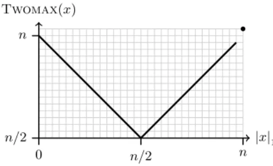
and Van Hoyweghen, Goldberg, and Naudts [5]. The function Twomax is es- sentially the maximum of Onemax and Zeromax . Local optima are solutions 0 ⁿ and 1 ⁿ where the number of zeros or the number of ones, respectively, is maximized. Hence, Twomax can be seen as a multimodal equivalent of One- max . The fitness landscape consists of two hills with symmetric slopes, i. e., an unbiased random search heuristic cannot tell in advance which hill is more promising. In contrast to [5, 13] we modify the function slightly such that only one hill contains the global optimum, while the other one leads to a local opti- mum. This is done by simply adding an additional fitness value for 1 ⁿ , turning it into a unique global optimum.

Let | x |

1

denote the number of 1-bits in x and | x |

0

the number of 0-bits in x.

Then for x = x

1

x

2

. . . x n

Twomax (x) := max {| x |

0

, | x |

1

} +

n

Y

i=1

x i .

Figure 1 shows a sketch of Twomax . Among all search points with more

than n/2 1-bits, the fitness increases with the number of ones. Among all search

points with less than n/2 1-bits, the fitness increases with the number of zeros.

Twomax (x)

|x|

₁

n/2

0 n

n/2 n

Figure 1: Sketch of Twomax . The dot indicates the global optimum.

We refer to these sets as branches and the algorithms as climbing these two branches of Twomax .

The Twomax function may appear in well-known combinatorial optimiza- tion problems. For example, the Vertex Cover bipartite graph analyzed in [11]

consists of two branches, one leading to a local optimum and the other to the minimum cover. In fact similar proof techniques as those used in this paper have also been applied in the vertex cover analysis of the (µ+1) EA for the bi- partite graph. Another function with a similar structure is the Mincut instance analyzed in [16].

Recombining individuals from different branches is likely to yield offspring of very low fitness. Since we are focusing on diversity for global exploration, we refrain from the use of recombination and only consider mutation-based EAs.

3 No Diversity Mechanism

In order to obtain a fair comparison of different diversity mechanisms, we keep one algorithm fixed as much as possible. The basic algorithm, the following (µ+1) EA, has already been investigated by Witt [18].

Alg. 1 : (µ+1) EA Let t := 0.

Initialize P

0

with µ individuals chosen uniformly at random.

Repeat

Choose x ∈ P t uniformly at random.

Create y by flipping each bit in x with probability 1/n.

Choose z ∈ P t with minimal fitness.

If f (y) ≥ f (z) then P t+1 = P t \ { z } ∪ { y } else P t+1 = P t .

Let t = t + 1.

The (µ+1) EA uses random parent selection and elitist selection for survival.

As parents are chosen randomly, the selection pressure is quite low. Neverthe-

less, the (µ+1) EA is not able to maintain individuals on both branches for

a long time. We now show that if µ is not too large, the individuals on one branch typically get extinct before the top of the branch is reached. Thus, the global optimum is found only with probability close to 1/2 and the expected optimization time is very large.

Theorem 1. The (µ+1) EA with no diversity mechanism and µ = o(n/log n) does not reach in polynomial time on Twomax the global optimum with proba- bility 1/2 − o(1). Its expected optimization time is Ω(n ⁿ ).

Proof. The probability that during initialization either 0 ⁿ or 1 ⁿ is created is bounded by µ · 2

⁻

ⁿ⁺¹ , hence exponentially small. In the following, we assume that such an atypical initialization does not happen as this assumption only introduces an error probability of o(1).

Consider the algorithm at a point of time t

^∗

where either 0 ⁿ or 1 ⁿ is created for the first time. Due to symmetry, the local optimum 0 ⁿ is created with probability 1/2. We now show that with high probability this local optimum takes over the population before the global optimum 1 ⁿ is created. Let i be the number of copies of 0 ⁿ in the population. From the perspective of extinction, a good event G i is to increase this number from i to i + 1. We have

P(G i ) ≥ i µ ·

1 − 1

n n

≥ i 4µ

since it suffices to select one out of i copies and to create another copy of 0 ⁿ . On the other hand, the bad event B i is to create 1 ⁿ in one generation. This probability is maximized if all µ − i remaining individuals contain n − 1 ones:

P(B i ) ≤ µ − i µ · 1

n < 1 n .

Together, the probability that the good event G i happens before the bad event B i is

P(G i | G i ∪ B i ) ≥ P(G i )

P(G i ) + P(B i ) . (1)

Plugging in bounds for P(B i ) and P(G i ) yields the bound i/(4µ)

i/(4µ) + 1/n = 1 − 1/n

i/(4µ) + 1/n ≥ 1 − 4µ in .

The probability that 0 ⁿ takes over the population before the global optimum is reached is therefore bounded by

µ

Y

i=1

P(G i | G i ∪ B i ) ≥

µ

Y

i=1

1 − 4µ

in

.

Using 4µ/n ≤ 1/2 and 1 − x ≥ e

^−2x

for x ≤ 1/2, we obtain

µ

Y

i=1

1 − 4µ

in

≥

µ

Y

i=1

exp

− 8µ in

= exp − 8µ n ·

µ

X

i=1

1 i

!

≥ exp( − O((µ log µ)/n))

≥ 1 − O((µ log µ)/n) = 1 − o(1).

Adding up all error probabilities, the first claim follows. If the population con- sists of copies of 0 ⁿ , mutation has to flip all n bits to reach the global optimum.

This event has probability n

⁻

ⁿ and the conditional expected optimization time is n ⁿ . As this situation occurs with probability 1/2 − o(1), the unconditional expected optimization time is Ω(n ⁿ ).

4 No Genotype Duplicates

It has become clear that diversity mechanisms are needed in order to optimize even a simple function such as Twomax . The simplest way to enforce diversity within the population is not to allow genotype duplicates. The following algo- rithm has been defined and analyzed by Storch and Wegener [14]. It prevents identical copies from entering the population as a natural way of ensuring di- versity. We will, however, show that this mechanism is not powerful enough to explore both branches of Twomax .

Alg. 2 : (µ+1) EA with genotype diversity Let t := 0.

Initialize P

0

with µ individuals chosen uniformly at random.

Repeat

Choose x ∈ P t uniformly at random.

Create y by flipping each bit in x with probability 1/n.

If y / ∈ P t then

Choose z ∈ P t with minimal fitness.

If f (y) ≥ f (z) then P t+1 = P t \ { z } ∪ { y } else P t+1 = P t .

Let t = t + 1.

We prove that if the population is not too large, the algorithm can be easily trapped in a local optimum.

Theorem 2. The (µ+1) EA with genotype diversity and µ = o(n

^1/2

) does not reach in polynomial time on Twomax the global optimum with probability 1/2 − o(1). Its expected optimization time is Ω(n ⁿ

⁻¹

).

Proof. We use a similar way of reasoning as in the proof of Theorem 1. With probability 1/2 − o(1), 0 ⁿ is the first local or global optimum created at time t

^∗

. Call x good (from the perspective of extinction) if | x |

1

≤ 1 and bad if | x |

1

≥ n − 1.

At time t

^∗

the number of good individuals is at least 1. In the worst case (again

from the perspective of extinction) the population at time t

^∗

consists of 0 ⁿ and µ − 1 bad individuals with n − 1 ones. Provided that the (µ+1) EA does not flip n − 2 bits at once, we now argue that the number of good individuals is monotone unless the unique 0-bit in a bad individual is flipped.

Due to the assumptions on the population only offspring with fitness at least n − 1 are accepted, i. e., only good or bad offspring. In order to create a bad offspring, the unique 0-bit has to be flipped since otherwise a clone or an individual with worse fitness is obtained. Hence the number of good individuals can only decrease if a bad individual is chosen as parent and its unique 0-bit is flipped. If there are i good individuals, we denote this event by B i and have P(B i ) = (µ − i)/µ · 1/n.

On the other hand, the number of good individuals is increased from i to i + 1 if a good offspring is created and a bad individual is removed from the population. We denote this event by G i . A good offspring is created with probability at least 1/(3µ) for the following reasons. The point 0 ⁿ is selected with probability at least 1/µ and then there are n − (i − 1) ≥ (e/3) · n 1-bit- mutations creating good offspring that are not yet contained in the population (provided n is large enough). Along with the fact that a specific 1-bit-mutation has probability 1/n · (1 − 1/n) ⁿ⁻¹ ≥ 1/(en), the bound 1/(3µ) follows. After creating such a good offspring, the algorithm removes an individual with fitness n − 1 uniformly at random. As there are i − 1 good individuals with this fitness and µ − i bad individuals, the probability to remove a bad individual equals (µ − i)/(µ − 1) ≥ (µ − i)/µ. Together,

P(G i ) ≥ 1

3µ · µ − i

µ = µ − i 3µ

²

.

Along with inequality (1), the probability that G i happens before B i is at least

µ

−

i

3µ²

µ

−

i

3µ²

+ ^µ _µn

⁻

ⁱ = 1

1 + 3µ/n = 1 − 3µ/n

1 + 3µ/n ≥ 1 − 3µ n .

The probability that the number of good individuals increases to µ before the global optimum is reached is

µ

Y

i=1

P(G i | G i ∪ B i ) ≥

1 − 3µ n

µ

≥ 1 − 3µ

²

n = 1 − o(1).

Adding up all error probabilities, the first claim follows.

The claim on the expected optimization time follows as the probability to create a global optimum, provided the population contains only search point with at most one 1-bit, is at most n

⁻⁽ⁿ⁻¹⁾

.

5 No Phenotype Duplicates

Avoiding genotype duplicates does not help much to optimize Twomax as indi-

viduals from one branch are still allowed to spread on a certain fitness level and

take over the population. A more restrictive mechanism is to avoid phenotype duplicates, i. e., multiple individuals with the same fitness. Such a mechanism has been defined and analyzed by Friedrich et al. [3] for plateaus of constant fitness.

The following (µ+1) EA with phenotype diversity avoids that multiple indi- viduals with the same fitness are stored in the population. If at some time step t, a new individual x is created with the same fitness value as a pre-existing one y ∈ P t , then x replaces y.

Alg. 3 : (µ+1) EA with phenotype diversity Let t := 0.

Initialize P

0

with µ individuals chosen uniformly at random.

Repeat

Choose x ∈ P t uniformly at random.

Create y by flipping each bit in x with probability 1/n.

If there exists z ∈ P t such that f(y) = f(z) then P t+1 = P t \ { z } ∪ { y } ,

else

Choose z ∈ P t with minimal fitness.

If f (y) ≥ f (z) then P t+1 = P t \ { z } ∪ { y } else P t+1 = P t .

Let t = t + 1.

From the analysis of Friedrich et al. [3] it can be derived that if the population size µ is a constant, then the runtime on a simple plateau is exponential in the problem size n. Only if µ is very close to n the expected runtime is polynomial.

In particular, if µ = n then the same upper bound as that of the (1+1) EA for plateaus of constant fitness [8] can be obtained (i. e., O(n

³

)). Probably, the phenotype diversity mechanism is not effective on simple plateaus. In the following, by analyzing the mechanism on Twomax , we show how also on a simple bimodal landscape, phenotype diversity does not help the (µ+1) EA to avoid getting trapped on a local optimum.

Since the diversity mechanism does not accept multiple individuals with the same fitness value, it does not make sense to have a population size that is greater than the number of different fitness function values. For the Twomax function this number is roughly n/2.

The following theorem proves that if the population is not too large, then with high probability the individuals climbing one of the two branches will be extinguished before any of them reach the top. Since the two branches of the Twomax function are symmetric, this also implies that the global optimum will not be found in polynomial time with probability 1/2 − o(1).

Theorem 3. The (µ+1) EA with phenotype diversity and µ = o(n

^1/2

) does

not reach in polynomial time on Twomax the global optimum with probability

1/2 − o(1). Its expected optimization time is n

^Ω(n)

.

Proof. We assume that the very unlikely situation that the global and the local optimum are created during initialization does not happen. As proved in previ- ous theorems such probability is exponentially small. We are interested in the first generation T

^∗

where the local optimum or the global one is created. The probability that the local optimum is created equals 1/2 due to the symmetry of the Twomax function.

Let individuals with i < n/2 zero-bits be called x i and ones with i < n/2 one-bits be called y i . Because of the phenotype diversity mechanism there may be only one x i or one y i in the population at the same time for i ≥ 1. Consider a situation where the local optimum y

0

= 0 ⁿ is reached before the global optimum and note that due to the phenotype diversity y

0

will remain in the population if µ ≥ 2. We will show that with probability 1 − o(1) the population { y

0

, . . . , y µ−1 } is created before the global optimum is found.

Then, if y i for i ≤ µ − 1 is chosen as parent, the minimum number of bits that have to flip in order to create some x i for i ≤ µ − 1 is n − 2n

^1/2

. This probability is at most

n 2n

^1/2

1 n

n−2n

^1/2

≤ 1

(n − 2n

^1/2

)! = n

^−Ω(n)

.

The probability that this happens at least once in n ^cn steps is still exponentially small if c > 0 is a small enough constant. This proves the claim on the expected optimization time.

It remains to be proved that the population { y

0

, . . . , y µ−1 } is reached with probability 1 − o(1). Let m be the smallest i such that y i+1 ∈ / P t . Note that m ≤ µ − 1. From the perspective of extinction, the following worst case population

P t = { y

0

, . . . , y m , x m+1 , . . . , x µ

−1

}

maximizes the probability of reaching the global optimum. We are optimistically assuming that the x-individuals are always one fitness level behind each other.

It may happen that the next step creates y m+1 . Then x m+1 is removed from the population and m increases by 1. Such a step is called a good step. Note that m is not changed if y m+i is created for i ≥ 2. For these steps, we pessimistically assume that the current population is still the worst case population. On the other hand, if x i for i ≤ m is created, then y i is removed and m decreases to i − 1. This is referred to as a bad step. All other steps lead us back to our worst case population.

We show that with high probability m increases to µ − 1 before a bad step happens. If x i is chosen as parent, a necessary condition for a bad step is that i − m out of i 0-bits flip. Hence the probability of a bad step is at most

µ

X

i=m+1

1 µ

i i − m

1 n

i

−

m

= 1 µ

µ−m

X

i=1

i + m i

1 n

i

≤ 1 µ

∞

X

i=1

µ n

i

≤ 1 µ · µ

n − µ = 1

n − µ ≤ 2

n ,

using µ = o(n

^1/2

) ≤ (1 − e/3)n < n/2 if n large enough. Hence, the probability of a good step is at least

1

µ · n − m en ≥ 1

µ · n − µ en ≥ 1

3µ

since it suffices to select y m and to flip exactly one out of n − m bits. So, the probability that a good step happens before a bad step is at least

1/(3µ)

1/(3µ) + 2/n = 1 − 1

n/(6µ) + 1 ≥ 1 − 3µ n .

The probability to increase m to µ − 1 by good steps before a bad step happens is bounded by

1 − 3µ

n ^µ

≥ 1 − 3µ

²

n = 1 − o(1), which concludes the proof.

Also if the population is larger than o(n

^1/2

) with probability 1 − o(1) the time to reach the global optimum is exponential in the problem size if the local optimum is found first. Drift analysis will be used to prove the above state- ment. This proof method was initially introduced by Hajek [6] and afterwards was extended to the run-time analysis of EAs by He and Yao [7]. A general description of the technique can be found in [12]. The following Drift theorem is a useful extension of the general proof method for proving run-time lower bounds that hold with exponentially high probabilities. Its first application can be found in [4].

Theorem 4 (Drift Theorem). Let X

0

, X

1

, X

2

, . . . be a Markov process over a set of states S, and g : S → R

⁺₀

a function that assigns to every state a non- negative real number. Pick two real numbers a(l) and b(l) which depend on a parameter l ∈ R

⁺

such that 0 < a(l) < b(l) holds and let the random variable T denote the earliest point in time t ≥ 0 where g(X t ) ≤ a(l) holds.

If there are constants λ > 0 and D ≥ 1 and a polynomial p(l) taking only positive values, for which the following four conditions hold

1. P(g(X

0

) ≥ b(l)) = 1 2. b(l) − a(l) = Ω(l)

3. ∀ t ≥ 0 : E[e

^{−λ(g(Xt+1)−g(Xt))}

| X t , a(l) < g(X t ) < b(l)) ≤ 1 − 1/p(l)]

4. ∀ t ≥ 0 : E[e

^{−λ(g(Xt+1)−b(l))}

| X t , b(l) ≤ g(X t )] ≤ D,

then for all time bounds B ≥ 0, the following upper bound on probability holds for random variable T

P(T ≤ B) ≤ e ^λ(a(l)

⁻

^b(l)) · B · D · p(l).

The following theorem proves exponential expected time for the (µ+1) EA with phenotype diversity on Twomax for any value of µ. We point out again that, given the diversity mechanism, it does not make sense to have a population size of µ > n/2.

Theorem 5. The (µ+1) EA with phenotype diversity does not reach in poly- nomial time on Twomax the global optimum with probability 1/2 − o(1). Its expected optimization time is e

^Ω(√3

ⁿ⁾ .

Proof. We pick up the line of thought from the proof of Theorem 3. With probability 1 − o(1), √

³

n + 1 = o(n

^1/2

) individuals y

0

, y

1

. . . y

^√3

_n are created before the global optimum is found. From the perspective of extinction the worst case population is P t = { y

0

, . . . , y

^√3

_n , x

^√3

_n+1 , . . . , x µ } . In the following we will use the drift theorem to prove that then with overwhelming probability it will take exponential time before the global optimum is created. Pessimistically arguing with worst-case populations as in Theorem 3 implies that the process we analyze drifts away from the optimum more slowly compared to the actual one.

Let X t be the population at time t and let g(X t ) denote the minimal Ham- ming distance of any individual in the population to the global optimum. Note that this distance corresponds to the number of 0-bits of the closest individual to the optimum and that it equals the value m + 1 from the proof of Theorem 3.

We define a(l) := 0 and b(l) := √

³

n + 1, that is, g(X t ) = a(l) = 0 contains the global optimum, while the population X t with g(X t ) = b(l) is √

³

n + 1 bits away.

With the µ − √

³

n − 1 individuals one fitness level behind each other, P(g(X

0

) ≥ b(l)) = 1 is satisfied. Also Condition 2 is satisfied since b(l) − a(l) =

√

3

n − 0 = Ω( √

³

n).

Conditions 3 and 4 still have to be proved to hold. Let p j := P(g(X t+1 ) − g(X t ) = j | X t , a(l) < g(X t ) < b(l)), then we rewrite Condition 3 as

1

X

j=−

√³

n

p j · e

⁻

^λj ≤ 1 − 1/p(l). (2)

A move with negative j is heading towards the optimum while one with positive j is drifting away. A move with j = 1 occurs if y g(X

t)−1

is selected as parent and exactly one out of n − (g(X t ) − 1) ≥ n − √

³

n zeros is flipped. Hence p

0

≤ 1 − p

1

≤ 1 − 1

µ · n − √

³

n

n ·

1 − 1

n n

−1

≤ 1 − 1 2eµ .

The probability of a step of length j ≥ 1 towards the optimum is maximal if g(X t ) = b(l) = √

³

n. A necessary condition is to choose x

^√3

_n+i and to create

x

^√3

_n−j by a step flipping i + j 0-bits for some i ≥ 0. Since (i +j)! ≥ (i + 1)! · j! ≥

((i + 1)/e) ⁱ⁺¹ · j!, we have

p

₋

j ≤ 1 µ

µ−

√³

n

X

i=0

i + √

³

n i + j

1 n

^i+j

≤ 1 µ

µ

−√³

n

X

i=0

i + √

³

n n

i+j

· 1 (i + j)!

≤ 1 µ · 1

j!

µ

−√³

n

X

i=0

i + √

³

n n

i+1

· 1 (i + 1)!

≤ 1 µ · 1

j!

µ

−√³

n

X

i=0

e(i + √

³

n) (i + 1)n

i+1

≤ 1 µ · 1

j!

µ

−√³

n

X

i=0

e √

³

n n

i+1

= 1 µ · 1

j! · O(n

^−2/3

).

As P

∞

j=0 e ^λj /(j!) = exp(e ^λ ),

√3

n

X

j=1

p

₋

j e ^λj = 1 µ ·

√3

n

X

j=1

e ^λj

j! · O(n

^−2/3

) ≤ 1

µ · e ^e

^λ

· O(n

^−2/3

).

Together, using the trivial bound p

1

≤ 1, the left-hand side of Inequality 2 is bounded by

e

⁻

^λ

µ + 1 − 1 2eµ + 1

µ · exp(e ^λ ) · O(n

^−2/3

)

= 1 − 1 µ

− e

^−λ

+ 1

2e − exp(e ^λ ) · O(n

^−2/3

)

≤ 1 − 1 p(l) if λ := 2, p(l) := 6n, and n is large enough.

The proof of condition 4 is easier. The following expectation has to be estimated:

∀ t ≥ 0 : E[e

⁻

^λ(g(X

^t+1)−

^b(n)) | X t , b(n) < g(X t )].

This is less or equal to:

E[e

⁻

^λ(g(X

^t+1)−

^g(X

^t))

| X t , b(n) < g(X t )] ≤

0

X

j=

−

n+(µ

−1)

r j · e

⁻

^λj

Here r j is the probability that the population X t at time step t such that b(l) < g(X t ) performs a step of length j. The probability of a move going towards the optimum is highest when the process is in position j = n − (µ − 1).

In this case the population is P t = { y

0

, y

1

. . . , y µ

−1

} . From this position no

moves may occur heading away from the optimum. We bound the sum as follows:

n−µ

X

j=0

r

₋

j · e ^λj ≤

∞

X

j=0

e ^λj n

j 1

n ^j ≤

∞

X

j=0

e ^λj

j! = exp(e ^λ ) < D

Since the inequality is satisfied for any constant λ and D large enough con- stant, condition 4 also holds.

Hence, the expected runtime is exponential (that is, e

^Ω(√3

ⁿ⁾ ) with overwhelm- ing probability for B = e ^c

^·

^l and c sufficiently small, since λ(a(l) − b(l)) =

− Ω( √

³

n).

6 Deterministic Crowding

In the deterministic crowding mechanism [10], offspring compete directly with their respective parents. In the following algorithm, an offspring replaces its parent if its fitness is at least as good.

Alg. 4 : (µ+1) EA with deterministic crowding Let t := 0.

Initialize P

0

with µ individuals chosen uniformly at random.

Repeat

Choose x ∈ P t uniformly at random.

Create y by flipping each bit in x with probability 1/n.

If f (y) ≥ f (x) then P t+1 = P t \ { x } ∪ { y } else P t+1 = P t .

Let t = t + 1.

The algorithm closely resembles a parallel (1+1) EA since µ individuals explore the landscape independently. However, interactions between the indi- viduals may be obtained by using other operators together with mutation. The crowding mechanism was introduced to guarantee diversity between individuals for the greater effectiveness of the recombination operator [10]. Recently, the mechanism together with crossover has proved to be useful in vertex cover prob- lems by making the difference between polynomial and exponential runtimes for some instances [11]. Here we concentrate on the capabilities of guaranteeing di- versity of the mechanism by analyzing the (µ+1) EA with deterministic crowd- ing on the Twomax function. For sufficiently large populations the algorithm can easily reach both local optima.

Theorem 6. The (µ+1) EA with deterministic crowding and µ = poly(n)

reaches on Twomax a population consisting of only local or global optima in

expected time O(µn log n). In that case the population contains at least one

global optimum with probability at least 1 − 2

⁻

^µ .

Proof. The main observation for the second statement is that the individuals of the population are independent due to the crowding mechanism. Due to the symmetry of Twomax , the i-th individual in the population reaches the global optimum with probability 1/2. The probability that at least one individual finds the global optimum is 1 − (1/2) ^µ .

Let T be the random time until all individuals have reached local or global optima on Twomax . It is easier to find a local optimum on Twomax than to find a global optimum on Onemax , hence we estimate E(T ) by the expected global optimization time on Onemax . Let P = { x

1

, . . . , x µ } and A i,j denote the event that the i-th 0-bit in x j is flipped by a 1-bit-mutation. (We do not consider fixed bit positions since mutation may turn a 1-bit to 0 and a 0-bit to 1, hence exchanging these two bits.) Clearly, all individuals in the population reach the optimum of Onemax within t steps if during this period A i,j happens for all 1 ≤ j ≤ µ and all 1 ≤ i ≤ | x j |

0

. In a single generation, we have P(A i,j ) ≥ 1/(enµ) (provided i ≤ | x j |

0

) since x j is selected for mutation with probability 1/µ and a specific 1-bit-mutation has probability at least 1/(en).

Let t := enµ(ln µ + ln n + ln 2). The probability that A i,j does not happen within t steps is bounded by

1 − 1

enµ

enµ(ln µ+ln n+ln 2)

≤ e

^−(ln

^{µ+ln n+ln 2)} = 1 2nµ .

By the Union bound, the probability that some event A i,j does not happen during t steps is at most 1/2. We conclude that after t steps all individuals reached the optimum with probability 1/2. In case this does not happen, we simply repeat the arguments with a new period of t steps. The expected number of periods is at most 2, yielding the bound E(T ) ≤ 2t = O(µn log n) since µ = poly(n).

7 Fitness Sharing

Fitness sharing (see, e. g., [10]) derates the real fitness of an individual x by an amount that represents the similarity of x to other individuals in the pop- ulation. The similarity between x and y is measured by a so-called sharing function sh(x, y) ∈ [0, 1] where a large value corresponds to large similarities and value 0 implies no similarity. The idea is that if there are several copies of the same individual in the population, these individuals have to share their fitness. As a consequence, selection is likely to remove such clusters and to keep the individuals apart. We denote the shared fitness of x in the population P as

f (x, P ) = f (x) P

y

∈

P sh(x, y) . The fitness of the population is then defined as

f (P ) = X

x

∈

P

f (x, P ).

It is common practice to use a so-called sharing distance σ such that individuals only share fitness if they have distance less than σ. Given some distance function d, a common formulation for the sharing function is

sh(x, y) = max { 0, 1 − (d(x, y )/σ) ^α }

where α is a positive constant that regulates the shape of the sharing function.

We use the standard setting α = 1 and set the sharing distance to σ = n/2 as this is the smallest value that still enables us to distinguish between the two branches. As Twomax is a function of unitation, we allow the distance function d to depend on the number of ones: d(x, y) :=

| x |

1

− | y |

1

. Such a strategy is known as phenotypic sharing [10]. Our precise sharing function is then

sh(x, y) = max (

0, 1 − 2

| x |

1

− | y |

1

n

) .

We now incorporate fitness sharing into the (µ+1) EA. Our goal is to evolve a good population, hence selection works by comparing candidates for next generation’s population w. r. t. their f (P)-values. This selection strategy has already been analyzed by Sudholt [15].

Alg. 5 : (µ+1) EA with fitness sharing Let t := 0.

Initialize P

0

with µ individuals chosen uniformly at random.

Repeat

Choose x ∈ P t uniformly at random.

Create y by flipping each bit in x with probability 1/n.

Let P _t

^∗

:= P t ∪ { y } .

Choose z ∈ P _t

^∗

such that f (P _t

^∗

\ { z } ) is maximized.

Let P t+1 = P _t

^∗

\ { z } and t = t + 1.

Note that when evaluating f (P _t

^∗

\ { z } ) the shared fitness values have to be recomputed for all these populations. However, with the use of dictionaries it suffices to compute f (y) and the sharing values sh(x, y ) for x ∈ P t only once.

We now show that the (µ+1) EA with fitness sharing can find both optima on Twomax . Imagining all parents and the new offspring on a scale of | x |

1

, the individuals with the smallest and the largest number of ones have the largest distance to all individuals in the population. Therefore, fitness sharing makes these outer individuals very attractive in terms of shared fitness, hence these individuals are taken over to the next generation. This even holds if an outer individual has the worst fitness in the population.

Lemma 1. Consider the (µ+1) EA with fitness sharing and µ ≥ 2 on Twomax . Let P _t

^∗

be the enlarged parent population at some point of time t and w. l. o. g.

let P _t

^∗

= { x

1

, . . . , x µ+1 } with | x

1

|

1

≤ | x

2

|

1

≤ · · · ≤ | x µ+1 |

1

. If | x µ |

1

< | x µ+1 |

1

then x µ+1 ∈ P t+1 . Also, if | x

1

|

1

< | x

2

|

1

then x

1

∈ P t+1 .

Proof. We only prove x µ+1 ∈ P t+1 for | x µ |

1

< | x µ+1 |

1

. The second claim for the case | x

1

|

1

< | x

2

|

1

follows by symmetry. Let P

⁻

:= P _t

^∗

\{ x µ+1 } , P

⁺

:= P _t

^∗

\{ x µ } and P

^∩

:= P

⁺

∩ P

⁻

. We will prove f (P

⁻

) < f (P

⁺

). This implies that P

⁻

does not have maximal population fitness among all possible next populations P _t

^∗

\ { z } examined in the selection step, hence x µ+1 remains in the population.

We first assume f (x µ ) ≤ f (x µ+1 ). Observe that sh(x µ , x) > sh(x µ+1 , x) for x ∈ P

^∩

due to the ordering of the x i and the definition of sh. Hence, P

y

∈

P

⁻

sh(x i , y) > P

y

∈

P

⁺

sh(x i , y) for x ∈ P

^∩

and P

y

∈

P

⁻

sh(x µ , y) >

P

y

∈

P

⁺

sh(x µ+1 , y). Together, we obtain f (P

⁻

) = X

x∈P

^∩

f (x) P

y∈P

⁻

sh(x, y) + f (x µ ) P

y∈P

⁻

sh(x µ , y)

< X

x

∈

P

^∩

f (x) P

y

∈

P

⁺

sh(x, y) + f (x µ+1 ) P

y

∈

P

⁺

sh(x µ+1 , y)

= f (P

⁺

).

It remains to show f (P

⁻

) < f (P

⁺

) for the case f (x µ ) > f (x µ+1 ). We want to examine the impact of the distance between the two individuals on the fitness and the sharing function. Therefore, we define

d ˜ := min n

| x µ+1 |

₁

, n 2

o − | x µ |

₁

.

Note that ˜ d ≥ 0 as | x µ |

1

≤ n/2 follows from f (x µ ) > f (x µ+1 ). The following two properties follow immediately from the definition of sh( · , · ) and f ( · ):

∀ x ∈ P

^∩

: sh(x, x µ+1 ) ≤ sh(x, x µ ) − 2 ˜ d

n , (3)

f (x µ ) − d ˜ ≤ f (x µ+1 ). (4) We will later also prove the following three inequalities:

∀ x ∈ P

^∩

: f (x, P

⁻

)

f (x, P

⁺

) ≤ 1 − 2 ˜ d

nµ (5)

f (x µ , P

⁻

)

f (x µ+1 , P

⁺

) < 1 + 2 ˜ d

nµ (6)

f (x µ+1 , P

⁺

) ≤ X

x∈P

^∩

f (x, P

⁺

) (7)

Using that all terms are positive, inequalities (5), (6), and (7) suffice to prove

our claim:

f (P

⁻

) = f (x µ , P

⁻

) + X

x∈P

^∩

f (x, P

⁻

)

< f (x µ+1 , P

⁺

) · 1 + 2 ˜ d nµ

!

+ X

x

∈

P

^∩

f (x, P

⁺

) · 1 − 2 ˜ d nµ

!

≤ f (P

⁺

) − 2 ˜ d nµ

X

x

∈

P

^∩

f (x, P

⁺

) − f (x µ+1 , P

⁻

)

!

≤ f (P

⁺

).

It remains to prove the inequalities (5), (6), and (7).

Proof of inequality (5): By inequality (3), f (x, P

⁻

)

f (x, P

⁺

) = P

y∈P

⁺

sh(x, y) P

y

∈

P

⁻

sh(x, y)

≤ P

y∈P

^∩

sh(x, y) + sh(x, x µ ) − 2 ˜ d/n P

y

∈

P

^∩

sh(x, y) + sh(x, x µ )

≤ µ − 2 ˜ d/n µ

using that the sharing function is at most 1. Reducing the last fraction by µ, inequality (5) follows.

Proof of inequality (6): By inequality (4) and f (x) ≥ n/2 for any x ∈ { 0, 1 } ⁿ , we have

f (x µ+1 )

f (x µ ) ≥ f (x µ ) − d ˜

f (x µ ) ≥ n/2 − d ˜

n/2 = 1 − 2 ˜ d n . Also, using inequality (3), we obtain

P

y

∈

P

⁺

sh(x µ+1 , y) P

y∈P

⁻

sh(x µ , y) = 1 + P

y

∈

P

^∩

sh(x µ+1 , y) 1 + P

y∈P

^∩

sh(x µ , y)

≤ 1 + P

y

∈

P

^∩

(sh(x µ , y) − 2 ˜ d/n) 1 + P

y

∈

P

^∩

sh(x µ , y)

≤ 1 + (µ − 1)(1 − 2 ˜ d/n)

µ . (8)

Taking the last two estimations together, f (x µ , P

⁻

)

f (x µ+1 , P

⁺

) = P

y∈P

⁺

sh(x µ+1 , y) P

y

∈

P

⁻

sh(x µ , y) · f (x µ ) f (x µ+1 )

≤ 1 + (µ − 1)(1 − 2 ˜ d/n) µ(1 − 2 ˜ d/n)

= 1 −

^{2 ˜}

n ^d + _nµ

^{2 ˜}

^d 1 −

^{2 ˜}

n ^d

< 1 + 2 ˜ d

nµ ,

which proves inequality (6).

Proof of inequality (7): First consider the right-hand side of inequality (7).

This term is minimized if all x ∈ P

^∩

equal x µ since then for all individuals in P

^∩

fitness is minimized and sharing is maximized. Along with f (x µ ) ≥ f (x µ+1 ),

X

x

∈

P

^∩

f (x, P

⁺

) ≥ (µ − 1) · f (x µ )

µ − 1 + (1 − 2 ˜ d/n) ≥ f (x µ+1 )

1 +

¹⁻

_µ−1

^{2 ˜}

^d/n . (9) Note that inequality (8) also implies P

y∈P

⁺

sh(x µ+1 , y) ≤ 1 + (µ − 1)(1 − 2 ˜ d/n).

Hence, the left-hand side of inequality (7) can be estimated by f (x µ+1 , P

⁺

) ≤ f (x µ+1 )

1 + (µ − 1)(1 − 2 ˜ d/n) . (10) Comparing the denominators of inequality (9) and inequality (10), inequality (7) follows since (µ − 1)

²

≥ 1.

Now it is easy to prove an upper bound on Twomax . To the best of our knowledge, the following theorem provides the first runtime analysis of an EA with fitness sharing for population sizes greater than 2.

Theorem 7. The (µ+1) EA with fitness sharing and µ ≥ 2 reaches on Twomax a population containing both optima in expected optimization time O(µn log n).

Proof. For a population P , we consider the following characteristic values as potential functions: m

0

(P) denotes the maximum number of zeros and m

1

(P) the maximum number of ones for the individuals in P . We are interested in the expected time until both potentials become n.

According to Lemma 1, both potentials are non-decreasing. If m

0

(P ) = k then we wait for an individual with k zeros to be chosen and for the number of zeros to be increased. The expected time for this to happen is bounded from above by O(µ · n/(n − k)). Hence, the expected time until the m

0

-potential reaches its maximum value n is O(µn log n). A symmetrical statement holds for the m

1

-potential, hence the expected time until both optima are found is O(µn log n).

8 Conclusions

We have examined the behavior of different diversity mechanisms on a fitness

landscape consisting of two hills with symmetric slopes. We rigorously proved

that without any diversification the (µ+1) EA is unable to climb up both hills

(Theorem 1). This still holds if we avoid genotype or phenotype duplicates. On

the other hand, stronger diversity mechanisms like fitness sharing and deter-

ministic crowding allow the (µ+1) EA to find both optima of our test function

Twomax with high probability. For fitness sharing we could prove this for ar- bitrary populations of size µ ≥ 2. For deterministic crowding, a slightly larger population is needed.

The work has also revealed important open problems. Theorems 1 and 2 apply only to sublinear population sizes. While experimental studies indicate similar results for larger populations, a theoretical analysis is difficult. It seems that a more thorough understanding of the long-term dynamics of genetic drift is required to strengthen the theorems.

References

[1] N. Chaiyaratana, T. Piroonratana, and N. Sangkawelert. Effects of diversity control in single-objective and multi-objective genetic algorithms. Journal of Heuristics, 13(1):1–34, 2007.

[2] S. Fischer and I. Wegener. The one-dimensional Ising model: Mutation versus recombination. Theoretical Computer Science, 344(2–3):208–225, 2005.

[3] T. Friedrich, N. Hebbinghaus, and F. Neumann. Rigorous analyses of sim- ple diversity mechanisms. In Proc. of GECCO ’07, pages 1219–1225, Lon- don, 2007. ACM Press.

[4] O. Giel and I. Wegener. Evolutionary algorithms and the maximum match- ing problem. In Proc. of STACS ’03, pages 415–426, London, UK, 2003.

Springer.

[5] D. E. Goldberg, C. Van Hoyweghen, and B. Naudts. From twomax to the Ising model: Easy and hard symmetrical problems. In Proc. of GECCO ’02, pages 626–633. Morgan Kaufmann, 2002.

[6] B. Hajek. Hitting-time and occupation-time bounds implied by drift anal- ysis with applications. Advances in Applied probability, 14:502–525, 1982.

[7] J. He and X. Yao. Drift analysis and average time complexity of evolution- ary algorithms. Artificial Intelligence, 127(1):57–85, 2001.

[8] T. Jansen and I. Wegener. Evolutionary algorithms: How to cope with plateaus of constant fitness and when to reject strings of the same fitness.

IEEE Transactions on Evolutionary Computation, 5(6):589–599, 2001.

[9] T. Jansen and I. Wegener. Real royal road functions: where crossover prov- ably is essential. Discrete Applied Mathematics, 149(1-3):111–125, 2005.

[10] S. W. Mahfoud. Niching methods. In T. B¨ack, D. B. Fogel, and

Z. Michalewicz, editors, Handbook of Evolutionary Computation, pages

C6.1:1–4. Institute of Physics Publishing and Oxford University Press, Bris-

tol, New York, 1997.

[11] P. Oliveto, J. He, and X. Yao. Population-based evolutionary algorithms for the vertex cover problem. Technical Report CSR-07-11, University of Birmingham, School of Computer Science, December 2007.

[12] P. S. Oliveto, J. He, and X. Yao. Computational complexity analysis of evolutionary algorithms for combinatorial optimization: A decade of re- sults. International Journal of Automation and Computing, 4(3):281–293, 2007.

[13] M. Pelikan and D. E. Goldberg. Genetic algorithms, clustering, and the breaking of symmetry. In Proc. of PPSN VI, pages 385–394, London, UK, 2000. Springer.

[14] T. Storch and I. Wegener. Real royal road functions for constant population size. Theoretical Computer Science, 320:123–134, 2004.

[15] D. Sudholt. Crossover is provably essential for the Ising model on trees. In Proc. of GECCO ’05, pages 1161–1167, Washington DC, 2005. ACM Press.

[16] D. Sudholt. Memetic algorithms with variable-depth search to overcome local optima. Technical Report CI-238/08, Collaborative Research Center 531, Technische Universit¨ at Dortmund, 2008.

[17] R. K. Ursem. Diversity-guided evolutionary algorithms. In Proc. of PPSN- VII, pages 462–471. Springer, 2002.

[18] C. Witt. Runtime analysis of the (µ+1) EA on simple pseudo-Boolean

functions. Evolutionary Computation, 14(1):65–86, 2006.