Single crystal growth and electron spectroscopy of d1-systems

Single crystal growth and

electron spectroscopy of d ¹ -systems

Inaugural-Dissertation Erlangung des Doktorgrades zur

der Mathematisch-Naturwissenschaftlichen Fakult¨at der Universit¨at zu K¨oln

vorgelegt von Holger Roth

aus Siegen

K¨oln 2008

Prof. Dr. L. H. Tjeng Prof. Dr. M. Gr¨uninger Tag der m¨undlichen Pr¨ufung:

15.02.2008

Contents

1 Introduction 1

2 Titanates: Basic Properties 5

2.1 Crystal Structure . . . 5

2.2 Magnetic Properties . . . 6

2.3 Electrical Transport Properties . . . 7

2.4 Band Gaps . . . 10

2.5 Band Structure . . . 12

2.6 Hubbard Model . . . 14

2.7 Crystal Field Splitting . . . 17

3 Crystal Growth 21 3.1 Zone Melting . . . 21

3.2 Floating Zone Furnace . . . 22

3.3 Stability of the Melting Zone . . . 24

3.3.1 Zone Length . . . 24

3.3.2 Stirring and Heat Profile . . . 24

3.3.3 Growth Rate . . . 26

3.3.4 Segregation Effects . . . 27

3.4 Educts . . . 29

3.4.1 Preparing the Feeding Rod . . . 31

3.5 NbO . . . 32

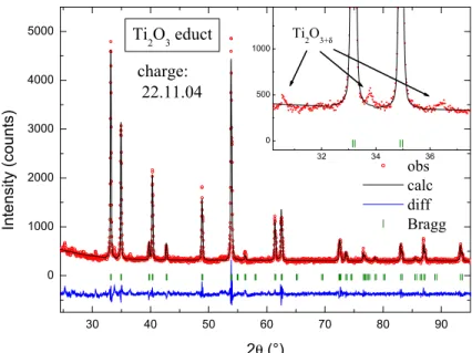
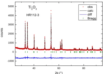
3.6 Ti2O3 . . . 35

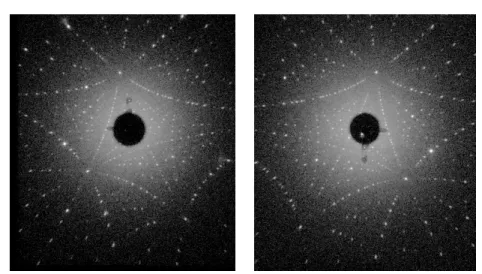
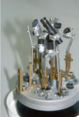
3.6.1 Single Crystallinity . . . 36

3.7 LaTiO₃ . . . 38

3.7.1 LaTiO_3+δ . . . 41

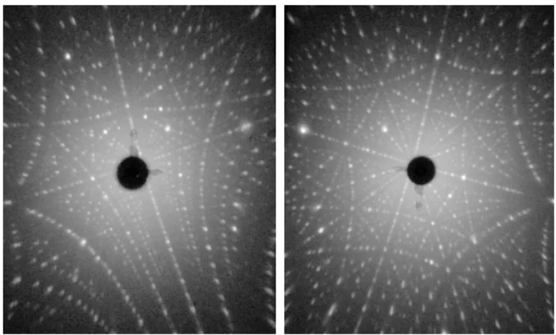
3.7.2 Single Crystallinity . . . 45

0.96 0.04 3

3.8 YTiO₃ . . . 54

3.8.1 Structural Phase Width and Oxygen Content . . . 55

3.8.2 Y_1−xCa_xTiO₃ . . . 60

3.9 GdTiO₃ . . . 64

3.9.1 Single Crystallinity . . . 67

3.10 SmTiO₃ . . . 67

3.10.1 Single Crystallinity . . . 69

3.11 NdTiO3 . . . 72

3.11.1 Single Crystallinity . . . 74

3.12 V_1−xCr_xO₂ . . . 75

3.12.1 Chromium Doping . . . 80

3.12.2 Single Crystallinity . . . 81

4 Photoelectron Spectroscopy 83 4.1 Theoretical Concept . . . 86

4.2 Bulk- vs Surface sensitivity . . . 87

4.3 Sample preparation and experimental setup . . . 95

5 Evolution of spectral weight 99 5.1 Introduction . . . 99

5.2 LaTiO₃ and YTiO₃: bulk-sensitive PES . . . 103

5.3 LaTiO₃ and YTiO₃: d¹ Spectral Weight . . . 105

5.4 La1−xSrxTiO3+δ: doping dependence . . . 109

Summary 115

Zusammenfassung 119

Acknowledgements 133

Publications 139

Chapter 1

Introduction

One of the most intriguing aspects of transition metal oxides is the wide variety and richness of their physical properties. They display quite often spectacular magnetic and electronic phenomena, including metal-insulator transitions (MIT), colossal magneto-resistance (CMR), superconductivity, spin-state transitions, magneto-optical activity and spin-dependent trans- port [1, 2]. Although conceptually simple and beautiful, theoretical sim- plifications in terms of, for instance, a Heisenberg model or a single band Hubbard model turn out to be inadequate [3–5]. It now becomes more and more clear that a full identification of the relevant charge, orbital and spin degrees of freedom of the metal ions involved is needed to understand the intricate balance between band formation and electron-correlation effects.

An important example is the manganates [6], where orbital ordering and charge distribution [7] of the Mn ions play an important role for its CMR behavior. For the newly synthesized layered cobaltates, it is the spin state transitions that are thought to govern the CMR and MIT phenomena [8,9].

Another example is V₂O₃ [10] and VO₂[11–13] for which it has been found that the orbital occupations across the various MITs change dramatically, leading to a switch of the nearest-neighbor spin-spin correlations so that in turn the effective band widths are strongly modified. This is surprisingly also the case for the ruthenates: here one would expect that the larger band widths of the 4dorbitals would make the system to be less correlated, but in reality the orbital switching across the metal-insulator [14–16] or magnetic phase [17] transitions is nevertheless no less dramatic. This indicates that not only electron-electron Coulomb repulsion, but also spin-spin correlations

must be considered in order to understand the transitions.

The class of the RETiO3 (RE = rare earth) materials forms in this context a very interesting ’playground’ for the quantitative study of the properties and excitation spectra of correlated oxides. It has the relatively simple perovskite crystal structure, and the Ti ions have (formally) only one electron in their 3d shell so that complications related to atomic mul- tiplet effects can be avoided. Yet, the orbital degeneracy together with the presence of a small band gap lead to a number of interesting physics which are then subject of a flurry of detailed experimental and theoretical studies.

Efforts are being made for a quantitative analysis as to test the accuracy of various theoretical approaches.

LaTiO3 is an antiferromagnetic insulator with a pseudocubic perovskite crystal structure [18–20]. The N´eel temperature varies between T_N = 130 and 146 K, depending on the exact oxygen stoichiometry [20–22]. Interest- ingly, a reduced total moment of about 0.45-0.57µ_Bin the ordered state has been observed [20–22]. One could speculate that this suggests the presence of an orbital angular momentum that is antiparallel to the spin momentum in the Ti³⁺ 3d¹ ion [22, 23]. Recently, however, Keimer et al.[24] have car- ried out neutron scattering experiments and observed that the spin wave spectrum of LaTiO₃ is nearly isotropic with a very small gap. They sug- gested that therefore the orbital momentum must be quenched. To explain the reduced moment, they proposed the presence of strong orbital fluctua- tions in the system. This seems to be supported by the theoretical study of Khaliullin and Maekawa [25], who suggested that LaTiO3 is in an orbital liquid state. This is a very exciting proposition, since if true, this would in fact constitute a completely novel state of matter.

Nevertheless, Cwik et al. [20], Mochizuki and Imada [26], as well as Pavarini et al. [27] estimated that small orthorhombic distortions present in LaTiO₃ would produce a crystal field (CF) splitting strong enough to lift the Ti 3d t_2g orbital degeneracy. Another theoretical study, however finds a much smaller CF splitting, leaving still open the possibility for an orbital liquid state [28]. The experimental determination of the magnitude of the CF splitting is difficult. Using soft-x-ray absorption spectroscopy at the Ti L2,3 edges as a local probe, Haverkort et al. [29] estimated that the CF splitting should be of order 0.12 – 0.30 eV. This value is large enough to prevent the formation of an orbital liquid. It is also large enough to strongly reduce the orbital moment from its ionic value, as found by the neutron

3

study by Keimer et al. [24] and also by the spin-resolved photoelectron spectroscopic experiment with circularly polarized light by Haverkort et al.

[29]. Nevertheless, the intriguing question remains whether one could find ways to modify LaTiO₃, for instance by doping or substitution, in order to minimize the influence of crystal fields and to generate orbital fluctuations.

In this respect it is interesting to note that the TN of the sample used in the neutron study [24] is less than optimal, opening the possibility that the sample is slightly off-stoichiometric and therefore, perhaps also slightly metallic. Would this cause sufficient charge fluctuations and, along with them, also orbital fluctuations? This issue is intimately connected to another aspect for which the titanates turned out to be an ideal model system for the study of the electronic structure of strongly correlated system, as described next.

One of the long standing topics in theoretical solid state physics con- cerns the single-particle spectral weight distribution in Mott-Hubbard sys- tems in the vicinity of the metal-insulator transition [2, 30]. The class of d¹ perovskites has been recognized in the last decade as a materializa- tion of this topic on which experimental tests can be carried out [31–37].

The comparative photoemission (PES) study on the band-width-controlled Ca_1−xSr_xVO₃material by Inoueet al.[34] yields striking systematic changes which triggered strong interest from the correlated electron community.

Also in the titanates one could observe very interesting features: upon doping, e.g. La1−xSrxTiO3, TN is quickly suppressed and new states are created in the vicinity of the chemical potential as seen by PES [31–37].

Somewhat surprising is that the doped system has an appreciable sharp Fermi cut-off, very much unlike magnetite in the metallic phase [38,39]. This seems to indicate that polaronic effects do not play a major role, making the system ideal to study the basics of the evolution of spectral weight in doped magnetic insulators without extra complications. Important is that the PES studies have found very heavy masses for the charge carriers in those doped titanates.

Nevertheless, the above mentioned photoemission results seem to be not consistent with data obtained from transport or thermodynamic mea- surements. Also the photoemission spectra of the undoped LaTiO₃ and YTiO₃ system cannot be reproduced by the various theoretical models presently available. There are now indications that those observations could be plagued by the surface sensitivity of the type of photoemission used in

those studies. It is being realized only in recent years, that the electronic structure of the surface of a material could be quite different from that of the bulk, especially for strongly correlated systems, in which the on-site and nearest neighbor interactions play the most relevant role. This is true not only for rare-earth intermetallics [40–44], but also for oxides. More recent PES studies using high photon energies to be more bulk sensitive [45,46], re- veal that for the Ca_1−xSr_xVO₃ system, the changes between bulk CaVO₃ and SrVO₃are too small to be detected. Also studies based on the dynami- cal mean field theories (DMFT) [47–50] indicate that the differences in band width are too small to have a noticeable impact on the spectra [27, 45, 51].

The objective of this thesis is to study the electronic structure of the ti- tanates as valuable model compound for a d¹ system, with emphasis on the evolution of the spectral weight as function of band width and doping. In view of the existing discussions in the literature, it is crucial to use better de- fined samples: we have to grow titanate single crystals with well defined sto- ichiometry and with well characterized magnetic and transport properties.

Another essential aspect of the work is to use photoelectron spectroscopy techniques which can deliver spectra which are truly representative for the bulk material. Only in this manner we can do a critical and quantitative evaluation of the various advanced many-body models currently available trying to describe the excitation spectra of strongly correlated systems.

The lay-out of the thesis is as follows:

We will start in chapter 2 with a description of the basic physical prop- erties of the titanates. A detailed description of the growth and character- ization of the samples will be given in chapter 3. Issues concerning photo- electron spectroscopy as a technique to measure the electronic structure will be explained in chapter 4. The results, including comparison with various theories, will be presented in chapter 5, followed by summary and acknowl- edgements.

Chapter 2

Titanates: Basic Properties

In this chapter we will describe several key physical properties of theRETiO₃ system. These include the crystal structure, electrical and magnetic prop- erties, as well as the basic electronic structure including crystal fields.

2.1 Crystal Structure

Like many chemical compounds with a AMX3 composition the RETiO3

crystallizes in the well known perovskite structure, which is shown in figure 2.1. Here the oxygen- together with the rare earth ions build a cubic closed package structure. The smaller Ti- ions are located in every fourth octahe- dral voids. These octahedra are connected with its six neighbors through corner sharing [53]. From this geometrical view ideal ratios of the ionic radii can be derived [53] for the structure to be cubic. The oxygen and rare earth ions should have the same size:

r_A=r_O, (2.1)

while the titanium ion must fit in the octahedral void and therefore must have as radiusr_{T i}:

r_{T i} =√ 2−1

r_O= 0.414r_O. (2.2) Deviations from this ratios can be treated by the tolerance factor of Goldschmidt [54]:

6 Titanates: Basic Properties

2.1 Perowskite

Perowskitverbindungen sind die h¨aufigsten Minerale der Erde. Sie verdanken ihren Namen einem Herrn Perowski aus St. Petersburg. Der eigentliche Perowskit ist CaTiO3, welches auch der erste Kristall war, der im Rahmen dieser Diplomarbeit erfolgreich pr¨apariert werden konnte (siehe Titelbild).

Chemische Verbindungen der allgemeinen Formel AMO3k¨onnen in der Perowskitstruktur kristallisieren. Auf den A-Pl¨atzen sitzen große Kationen, h¨aufig Erdalkali-, Seltenerd- oder Yttriumionen. Bei den Ionen, die die M-Pl¨atze einnehmen, handelt es sich meist um Katio- nen der ¨Ubergangsmetalle. Die Struktur des idealen Perowskits wird mit der Raumgruppe Pm3m beschrieben. In Abb. 2.1 ist die ideale Perowskitstruktur dargestellt. In den Ecken

(a) Eckenverkn¨upfte TiO6-Oktaeder. (b) Kubisch dichte Kugel- packung der violett gekenn- zeichneten Sauerstoff- und Kalziumionen.

Abbildung 2.1: Elementarzelle des kubischen Perowskits

der Elementarzelle sitzen die kleinen M-Kationen. Sie sind jeweils von 6 Sauerstoffionen

7

Figure 2.1: The cubic perovskite structure. In the left picture is the focus on the network of corner shared octahedra and in the right on the cubic closed ball package of the oxygen and Ca ions in the perovskite structure.

to illustrate the ccp structure the 12 neighbor atoms of the Ca ion colored purple from [52].

t= √r_RE+r_O

2 (r_{T i}+r_O). (2.3)

Fort <0.96 the octahedra become tilted against each other, what leads to the GdFeO₃structure which is shown in figure 2.2 with the corresponding space group Pbnm [55,56]. This is the structure of the RETiO3compounds.

In the observed rare earth series the radius of the trivalent ions gets smaller with its atomic number and is smallest for the Gd³⁺ and Y³⁺ ions.

This is connected with an increasing tilt of the Ti-O-Ti bond angle θ. For the compound with the largest rare earth ion, namely LaTiO₃, the bond angle isθ≈155^◦ while for the YTiO3the bond angle is reduced to an value of ≈142^◦ [18–20,57].

2.2 Magnetic Properties

The RETiO3 materials order magnetically. LaTiO3, for example, is a G- type antiferromagnet with a N´eel temperature which varies between T_N = 130 and 146 K, depending on the exact oxygen stoichiometry [18, 20–22].

YTiO3 on the other hand, is a ferromagnet with a Curie temperature of about T_C = 29 K [18,58].

2.3 Electrical Transport Properties 7

Figure 2.2: GdFeO3 unit cell; the orange cube in the middle shows the unit cell of the cubic perovskite.

Figure 2.3 shows the magnetic phase diagram ofRETiO₃ as a function of the rare-earth ionic radius [57]. One can clearly see that the crossover be- tween ferromagnetic and antiferromagnetic order is linked to the size of the rare-earth ion. This in turn, as we will see later, determines the crystal field levels and consequently the orbital occupations governing the sign and mag- nitude of the superexchange interactions via the Goodenough-Kanamori- Anderson rules [62–64].

2.3 Electrical Transport Properties

Temperature dependent resistivity measurements on the La_1−xSr_xTiO_3+δ and Y_1−xCa_xTiO₃ series show that the parent LaTiO₃ and YTiO₃ com- pounds are essentially insulators [60, 65]. It is only upon doping with Sr, Ca or excess of oxygen that the material acquire a metallic-like behavior as indicated by the positive resistivity-temperature slopes as displayed in fig- ure 2.4. Here one must note that the oxygen content in the La(Sr)-titanates is a parameter which is difficult to control, and yet very important for the

The high-field effects have to be considered as an enhance- ment of the integrated zero-field thermal-expansion anoma- lies, as can be seen in Fig. 6 共 a 兲 . At zero field the ferromag- netic ordering in YTiO

₃

is accompanied by a small antiferromagnetic moment along the a axis due to the com- peting magnetic interactions,

⁵⁰

which are determined through the orbital arrangement. Upon cooling in zero field, the or- bital arrangement is changing in the way that ferromag- netism is further stabilized; this effect seems to be further strengthened by the external field which anyway stabilizes the ferromagnetic order.

E. Crystal structure across theRTiO₃ series

Figure 7 shows the magnetic phase diagram of RTiO

₃

as a function of the rare-earth ionic radius. In addition to the pure RTiO

₃

samples we have included results on samples where the A site is occupied by a mixture of La and Y. The diagram clearly shows how the crossover from ferromagnetic to anti- ferromagnetic order is driven by the rare-earth ionic radius, even though some influence of additional effects is visible. In the ferromagnetic RTiO

₃

, there is a stronger variation of the Curie temperature which indicates the direct influence of the R-Ti magnetic interaction. Nonmagnetic Y implies a compa- rably low Curie temperature in this series. Nevertheless, the rare-earth ionic radius can be considered as the main external parameter driving the magnetic transition in the pure, as well as in the mixed compounds.

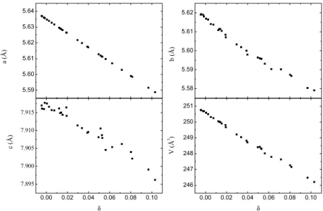
In Fig. 8 the results of our single-crystal diffraction mea- surements performed at room temperature are resumed.

Qualitatively, these results agree with previous studies,

⁴

but

there are significant quantitative differences due to the im- proved sample quality and due to he higher precision ren- dered possible with modern CCD x-ray techniques.

Both NdTiO

₃

crystals with T

_N

of 94 K and of 81 K were studied at room temperature. The lower T

_N

of the second crystal already indicates some nonstoichiometry. With x-ray diffraction it is difficult to determine precisely the oxygen content; therefore, it is not astonishing that the change in the refined oxygen content per formula unit from 2.952 共 30 兲 共 high-T

_N

sample 兲 to 2.988 共 12 兲 共 low-T

_N

sample 兲 is not very significant. However, in the low-T

_N

sample we find a signifi- cant amount of vaccancies on the Nd site with a content per formula unit of only 0.979 共 1 兲 , whereas the high-T

_N

sample as well as the other RTiO

₃

compounds with high transition tem- peratures show the ideal R to Ti ratio within comparable precision. The structural parameters obtained for the low-T

_N

and high-T

_N

samples are comparable in view of the large variation of the internal parameters in the RTiO

₃

series 共 see Table I 兲 ; however, clear differences can be detected. The main influence of the excess oxygen consists in a reduction of the octahedron tilting. Since excess oxygen and Nd vacan- cies enhance the Ti valence and thereby reduce the effective Ti-ionic radius, this tilt reduction is in perfect agreement with the bond-length mismatch scenario described by the tolerance factor. A similar suppression of the tilt distortion by excess oxygen was also found in La

₂

CuO

_4+␦

.

⁵¹

The enhanced Ti valency in the nonstoichiometric sample is directly ob- served in the bond-valence sum which is 0.045 共 1 兲 larger than that in the stoichiometric compound.

In Fig. 8 we plot the structural parameters against the rare-earth ionic radius. The largest overall structural changes concern the tilt and rotation deformations. The decrease of the rare-earth ionic radius enhances the bond-length mis- match and these angles, as seen in Fig. 8 共 a 兲 and in the Ti- O-Ti angles shown in Fig. 8 共 b 兲 . The distortion of the ideal perovskite structure gets extremely strong for YTiO

₃

which appears close to the stability of the Pbnm structure. Due to

FIG. 7.

共

Color online

兲

Magnetic phase diagram for RTiO₃ and La_1−xY_xTiO₃. T_C and T_N are plotted as a function of the rare-earth ionic radius. Squares: T_C, T_N for RTiO₃ from this work. Triangles:

values for RTiO₃ from Greedan

共

Ref. 33

兲

. Crosses: values for RTiO₃ from Katsufuji et al.

共

Ref. 55

兲

. Circles: values for La_1−xY_xTiO₃ from Okimoto et al.

共

Ref. 3

兲

. Stars: values for La_1−xY_xTiO₃ from Goralet al.

共

Ref.56

兲

. The insets show the prin- cipal octahedral deformations of the end members.

FIG. 6.

共

Color online

兲 共

a

兲

Thermal expansion

␣

^{= 1 /l}⳵l/⳵T of YTiO₃ for various magnetic fields as a function of temperature

共

H储a

兲

.

共

b

兲

Magnetostriction ⌬L

共

H

兲

/L of YTiO₃ as a function of applied magnetic field H储a.

224402-8

Figure 2.3: Magnetic phase diagram for RETiO₃ and La_1−xY_xTiO₃taken from [57]. TcandTN are plotted as a function of the rare-earth ionic radius.

Squares: T_c and T_N for RETiO₃ from this work. Triangles: values for RETiO₃ from Greedan [59]. Crosses: values for RETiO₃ from Katsufujiet al. [60] Circles: values for La1−xYxTiO3 from Okimoto et al. [35]. Stars:

values for La_1−xY_xTiO₃from Goralet al.[61]. The inset shows the principal octahedra of the end members.

properties of the material. Not only has a slight oxygen off-stoichiometry a strong reduction effect on the N´eel temperature of LaTiO₃ [18,20–22], but it also drives the material quickly away from its insulating character. This is demonstrated in figure 2.5, where one can observe that δ=0.01 is already sufficient to make LaTiO_3+δ to have a temperature independent resistivity curve. One really needs to have δ values much smaller than 0.01 to find a clear insulating behavior.

2.3 Electrical Transport Properties 9

Figure 2.4: Temperature dependence of the resistivity for LaTiO_3+δ or La1−xSrxTiO3 and for Y1−xCaxTiO3 from [60,65].

74 Kapitel 7 Pr¨aparierte Kristallsysteme

20 40 60 80 100 120 140 160 180 200 220 240 260 280 300 320 10^-7

10^-6 1x10^-5 1x10^-4 10^-3 10^-2 10^-1 10⁰ 10¹ 10² 10³ 10⁴ 10⁵ 10⁶

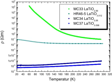
MC33 LaTiO_2.99 HR46-5 LaTiO_3.012 MC34 LaTiO_3.06 MC37 LaTiO_3.098

ρ (Ωm)

Temperatur (K)

Abbildung 7.23: Spezifischer Widerstand ρ in Abh¨angigkeit des Sauerstoffgehalts. MC34, MC33 MC37 wurden von K. Kordonis und HR46 von A. El Filali gemessen.

7.5 La

1−x

Sr

x

TiO

3+δ

7.5.1 Pr¨aparation

Zus¨atzlich zu den Edukten f¨ur die Pr¨aparation von LaTiO3+δ wurde außerdem noch das Oxid SrO der Firma Johnson Matthey GmbH verwendet. Nach der Reaktionsgleichung:

SrO + TiO2−→SrTiO3 (7.6)

sollen diese Oxide zu Strontiumtitanat reagieren, so dass die Gesamtreaktion lautet:

(1−x) (La2O3+ Ti2O3)

| {z }

La Ti O3

+ 2x| (SrO + TiO{z 2})

Sr Ti O3

−→2La1−xSrxTiO3. (7.7)

Bei einer ersten Pr¨aparation von La0.75Sr0.25TiO3wurde wie in [57] vorgegangen. Keim und Barren wurden zuerst vorreagiert und gesintert. Anschließend wurden beide in ¨ublicher Weise im Spiegelofen montiert.

Als Zuchtparameter wurde eine Argonatmosph¨are von 2 bar bei einer Flussrate von 1 l/min gew¨ahlt. Selbst eine Leistung von 4·1000 Watt, also die maximale Leistung des verwen- deten Lampensatzes, reichte nicht aus, um den Barren aufzuschmelzen. Auch drastisches Herabsetzen des Atmosph¨arendrucks und der Durchflussrate, um einerseits den Schmelz- punkt zu erniedrigen und andererseits eine k¨uhlende Wirkung des str¨omenden Gases zu minimieren, brachte keinen Erfolg. Weitere Pr¨aparationsversuche von La0.75Sr0.25TiO3und La0.9Sr0.1TiO3 dieser Art blieben ebenso erfolglos.

Bei einer weiteren Pr¨aparation von La0.9Sr0.1TiO3wurden zun¨achst die 4·1000 Watt Lam- pen in den doppelfokussierenden Spiegeln des Zonenschmelzofens neu fokussiert. Außerdem

Figure 2.5: Resistivity of the Sr-doped LaTiO₃ system [52].

Figure 2.6: Spectra of optical conductivity in La_1−xY_xTiO₃ at room temperature. A crossing point of a baseline and a dashed line is defined as the Mott-Hubbard gap energy. Taken from [35].

2.4 Band Gaps

With the resistivity experiments indicating the insulating nature of the un- doped or parent titanates, e.g. LaTiO3 and YTiO3, it is then natural to raise the question about the size of the conductivity gap. This is im- portant for the understanding and modelling of the electronic structure of the material as we will see later. Figure 2.6 show the optical conductivity of LaxY1−xTiO3 measured by Okimoto et al. [35]. For the pure YTiO3

(x=0), one can clearly see that the onset of strong absorption is located at about 0.6 eV photon energy. This can be identified as the band gap value.

For LaTiO3 (x=1) however, the situation is somewhat unclear. One does not observe a smooth onset but rather a bump centered at about 0.3 eV.

The origin of this bump is not clear, and it has been speculated that this is caused by slight oxygen off-stoichiometry. Nevertheless, if one is willing to make an extrapolation from the range between 0.8 and 1.4 eV, then a value of about 0.2 eV can be found for which the optical conductivity vanishes.

More recent optical data are provided by R¨uckamp et al., see Figure 2.7.

Also here one can deduce a band gap value of 0.6 eV for YTiO₃ by taking

2.4 Band Gaps 11

17

_InstituteofPhysics

⌽

DEUTSCHE PHYSIKALISCHE GESELLSCHAFT

0.2 0.4 0.6 0.8 1.0

0 5 10

SmTiO₃ (+2/Ωcm)

YTiO₃

LaTiO₃ T = 4 K

σ(ω) (1

/

Ωcm)

Energy (eV)

Figure 6.

Optical conductivity of (twinned) single crystals of LaTiO

₃

, SmTiO

₃

and YTiO

₃

at T = 4 K. An offset of 2

⁻¹

cm

⁻¹

has been added to the data of SmTiO

₃

for clarity. Phonon-activated orbital excitations are observed at 0.3 eV in all three compounds. For LaTiO

₃

, an estimate of the orbital excitation band has been obtained by subtracting a linear background (- - - -). The additional sharp features in SmTiO

₃

at 0.15, 0.3 and 0.45 eV are due to crystal-field transitions within the Sm 4f shell [111].

been proposed that the transition from antiferromagnetic order to ferromagnetic order should define a quantum critical point. SmTiO

₃

is still antiferromagnetic, but lies close to the critical value of the ionic radius [113]. By measuring both the transmittance and the reflectance on twinned single crystals, we were able to observe phonon-activated orbital excitations in LaTiO

₃

, SmTiO

₃

and YTiO

₃

at about 0.3 eV, i.e. in the frequency range between the phonons and the band gap (see figure 6). In YTiO

₃

, the Hubbard gap can be identified with the onset of strong absorption at about 0.6 eV. In LaTiO

₃

, the optical conductivity shows strong absorption above 0.8 eV, but an absorption tail extends down to about 0.2 eV. In a recent LDA+DMFT study, the Hubbard gap of LaTiO

₃

(YTiO

₃

) was reported to be 0.3 eV (1 eV) [48]. This issue of the onset of interband excitations will be discussed elsewhere. Here, we focus on the weak absorption features at about 0.3 eV observed in LaTiO

₃

, SmTiO

₃

and YTiO

₃

.

An interpretation in terms of phonons can be excluded since phonon absorption is restricted to below ≈ 80 meV. The small peak in YTiO

3

at about 160 meV typically marks the upper limit for two-phonon absorption in transition-metal oxides with perovskite structure [51]. Absorption of three or more phonons has to be much weaker. According to the magnon energies observed by inelastic neutron scattering [31, 114], the energy of 0.3 eV is much too high also for phonon- assisted magnetic absorption (i.e. two magnons plus a phonon [72, 73]). The very sharp additional absorption lines observed in SmTiO

3

at about 0.15, 0.3 and 0.45 eV are attributed to crystal- field transitions within the Sm 4f shell [111]. These lines are much narrower than the d–d bands, because in case of the 4f levels both the coupling to the lattice and the coupling between nearest-neighbour sites are much smaller.

New Journal of Physics 7(2005) 144 (http://www.njp.org/)

Figure 2.7: Optical conductivity of (twinned) single crystals of LaTiO₃, SmTiO₃ and YTiO₃ at T = 4 K. An offset of 2 Ω⁻¹ cm⁻¹ has been added to the data of SmTiO3 for clarity. Phonon-activated orbital excitations are observed at 0.3 eV in all three compounds. For LaTiO₃, an estimate of the orbital excitation band has been obtained by subtracting a linear background (- - - -). The additional sharp features in SmTiO3 at 0.15, 0.3 and 0.45 eV are due to crystal-field transitions within the Sm4f shell [111], taken from [66].

the onset of strong absorption. The LaTiO₃ spectrum shows surprisingly also a bump at about 0.3 eV, similar to the Okimoto data, although here great efforts were made to secure the stoichiometry of the sample. This lead R¨uckamp et al. to conclude that the 0.3 eV gap originates fromd−dexci- tations associated with the crystal field splitting of the Ti 3d orbitals [66].

Yet, it is not clear from this spectrum what the band gap of LaTiO3 should be.

2.5 Band Structure

Electronic structure calculations are indispensable for a better understand- ing of the physical properties and correct interpretation of the experimental data. This is especially true for transition metal oxides in which the cor- related motion of the electrons more than often is cause for unexpected entanglement of competing interactions. We will use the ab-initio density functional theory (DFT) within the local density approximation (LDA) as a first step to obtain a general orientation on the relationship between crystal structure, chemical composition and basic electronic structure features such as the one-electron band widths and crystal fields.

Various groups have calculated the band structure of the RETiO₃ sys- tem with very consistent results [27,31–33,37,67–69]. The basic features are shown for LaTiO₃ and YTiO₃in figures 2.8 and 2.9 as reproduced from the work by Pavarini et al. [71]. The O 2p derived bands are located between -3 eV and -8 eV energy indicating that the O 2p bands are essentially full, i.e. complying with the O²⁻ formal valence. The Ti 3dbands can be found between -1 eV and +6 eV energy, whereby the lower lying parts (i.e. between -1 eV and +1 eV) are built up from thet2g orbitals and the higher lying parts from the e_g orbitals. The La 5dand Y 4d like bands are positioned above the Fermi level, reflecting their trivalent ionic states.

In comparing the band structures calculated for the hypothetical ideal cubic structure and for the real structures, one notices immediately that the bands become narrower. This is not only true for the O 2p bands, but also for the Ti 3d, whereby the band narrowing even results in an opening of a gap between thet_2g ande_gbands. Important also is to notice that the bands of the YTiO₃ are narrower than those of the LaTiO₃, consistent with the larger distortions and tilts of the TiO6 octahedra in the Y system.

The most striking result of the LDA calculations is that Ti 3d-t_2g bands straddle through the Fermi level giving the prediction that LaTiO3 and YTiO₃ are metallic. This is clearly a failure. The insulating nature of the materials as found from resistivity measurements is not explained by the calculations. The sizable 0.6 eV band gap as observed clearly by optical spectroscopy for YTiO₃ is not at all reproduced. The implications of this failure are far reaching. It can be taken as a direct evidence for the strongly correlated motion of the electrons in these materials, calling for a quite different approach for the description for their electronic structure.

2.5 Band Structure 13

0 0 8

4

0

-4

-8

Energy [eV]

Figure 2.8: Crystal structures and electronic bandstructures for the3d(e_g) orthorhombic perovskites LaTiO3 and YTiO3: A (green), B (red) and O (blue). The bottom part shows densities of one-electron states (DOSs) cal- culated in the LDA for the real structures (right-hand panels) and for hy- pothetical, cubic structures with the same volumes (left-hand panels). The green, red, and blue DOSs are projected onto, respectively, (La, Y)d, Ti3d, and O 2p orthonormal orbitals [70]. The Ti3d(t_2g) bands are positioned around the Fermi level (zero of energy) and their widths, W, decrease from

∼ 3 to ∼ 2 eV along the series. The much wider Ti3d(eg) bands are at higher energies. This figure resulted from linear muffin-tin orbitals (LMTO) calculations in which the energies, _νRl, of the linear, partial-wave expan- sions were chosen at the centers of gravity of the occupied, partial DOS.

Since those energies are in the O 2p band, the LMTO errors proportional to (ε−_νRl)⁴ slightly distort the unoccupied parts of the DOS.

10 _InstituteofPhysics

⌽

DEUTSCHE PHYSIKALISCHE GESELLSCHAFT

Figure 4. LDA bandstructure of orthorhombic LaTiO3. The BZ is shown in red in figure9. The bands obtained with the truly minimal (downfolded) O 2pNMTO basis (red) are indistinguishable from those obtained with the full NMTO basis (black). This is explained in appendix A. The basis functions of the truly minimal set are shown in figures5and6. The recent structural data [12] was used.

It is well accepted that equilibrium crystal structures, such as those shown at the top of figure1, may be computedab initiowith good accuracy using the LDA. In the bottom right-hand panels we therefore show the LDA densities of states (DOS) calculated for the real structures—

determined experimentally though [20], [42]–[44]—and in the bottom left-hand panels we show the LDA DOS calculated for hypothetical, cubic structures with the same volume. Now, the energy gain associated with a structural distortion is approximately the gain in band-structure plus Madelung energy, so let us consider the trend in the former.

For SrVO₃the left- and right-hand panels are identical because the real structure of SrVO₃is cubic. Each Sr ion is at the corner of a cube and has 12 nearest oxygens at the face centres. Going now to cubic CaVO3the empty 3dband of Ca lies lower and thereby closer to the oxygen 2pband than the empty 4d band of Sr. It is therefore conceivable that a GdFeO3-type distortion which pulls some of the oxygen neighbours closer to the A ion and thereby increases the covalency with those, is energetically more favourable in CaVO3than in SrVO3, and this is what the figure shows: an increase of the O 2p–Ca 3d gap associated with the distortion in CaVO₃. The Ca 3d character is essentially swept out of the lower part of the V 3d band.

When proceeding to the titanates, the A and B cations become 1st- rather than 3rd- nearest neighbours in the periodic table. The B 3d band therefore moves up and the A d band down with respect to the Op band. Hence, the O-B covalency decreases and the O-A covalency increases. Most importantly, the Adband becomes nearly degenerate with the Ti 3d band, and more so for Y 4d than for La 5d. It is only the GdFeO₃-distortion which, through increase of the O 2p-Ad hybridization, pushes the Ad band above the Fermi level. This, as

New Journal of Physics 7(2005) 188 (http://www.njp.org/)

Figure 2.9: LDA bandstructure of orthorhombic LaTiO₃. The bands obtained with the truly minimal (downfolded) O2p NMTO basis (red) are indistinguishable from those obtained with the full NMTO basis (black), from [71].

2.6 Hubbard Model

The failure of the band structure calculations to describe the insulating state of the titanates can be traced back to the neglect of the strong on-site Coulomb interaction in the Ti 3dshell. In conventional band-structure the- ory, every electron is presumed to move independently through a periodic potential dictated by the positive ion cores that make up the lattice, and the collective potential of all the other electrons together in a mean-field manner.

These effectively single-particle theories work actually surprisingly well to describe large classes of solids, mostly wide band materials like semiconduc- tors and many common metals. But for transition metal oxides, including the titanates, the electron-electron repulsion at the transition metal sites are so strong that their effect have to be taken into account in an explicit manner.

2.6 Hubbard Model 15 1.5. Coulomb interaction and Mott-Hubbard insulators 11

Consider the following ground-state system in the tight-binding limit, consisting of

M

sites, in which every site has

n

electrons, for a total of

N

electrons in the whole system:

n n n n n n n

For the moment we leave out the electron spin and consider each site as consisting of a single infinitely-degenerate orbital. Moving an electron from one site to another site far away, i.e., creating a non-local electron-hole pair, leaves us with

n n

−1

n n n n

+1

n

The total Coulomb energy in the initial state is

M·¹₂n(n−

1)U , while in the final state it is (M

−

2)·

¹₂n(n−1)U

+

¹₂

(n

−

1)(n

−

2)U +

¹₂

(n +1)nU . It is easy to work out that, whatever the ground-state occupation

n

is, the difference between the initial and final state, and thus the creation energy of an electron-hole pair, is always equal to

U

.

To determine the magnitude of

U, the process of creating an electron-hole

pair can be split up into two independent actions, namely removing an electron (which costs the ionization energy

EI

), and adding an electron somewhere else (which gains the electron affinity

EA

). The pair interaction

U

is then equivalent to the difference

E_I−E_A

. These two processes, which create, respectively, an

N −

1 and an

N

+ 1 electron system, are commonly called photoemission and inverse photoemission processes.

An interesting question is now whether this “correlation” energy

U

, that is not present in one-electron theories, may completely inhibit the movement of electrons (and hence cause the system to become insulating) under certain circumstances, even in a system that is not comprised of closed-shell atoms or molecules (and so, classically, would be a metal). One of the simplest models used to address this problem, for an array of atoms with only

s-orbitals, is the

Hubbard model [53–55], described by the Hamiltonian

H

=

−t

i,j,σ

(c

^†_iσcjσ

+

c^†_jσciσ

) +

U

i

ni↑ni↓,

where

t

is the hopping integral (which is assumed to be equal for all sites),

c^†_iσ

and

c_iσ

are the creation and annihilation operators for an electron at site

i

with spin

σ

(↑ or

↓),niσ

=

c^†_iσciσ

is the number operator, and

i, j

signifies a sum over nearest-neighbours. The general solution of this model is unknown except in one dimension, and even there it is far from trivial, so we will not go very deeply into

To illustrate the basic features of a strongly correlated system, let us consider the case of the so–called Hubbard model. This model consists off- fold degenerate orbitals at each atomic site and electrons can hop from site to nearest-neighbor site with transfer integral t. In the absence of electron- electron interactions, this will result in a total band widthW =ZtwhereZis a parameter proportional to the coordination number, andW is then called the one-electron band width. Electron-electron interactions can then be introduced in the form of a Coulomb repulsion between pairs of electrons on one atom, and is indicated by the quantityU, often also called the Hubbard U. The pair interaction U can be shown to be equivalent to the energy it costs to move an electron from one part of the system to another, over a large distance.

Consider the following ground-state system in the tight-binding limit, consisting of M sites, in which every site has n electrons, for a total of N electrons in the whole system: For the moment we leave out the electron spin and consider each site as consisting of a single infinitely-degenerate orbital.

Moving an electron from one site to another site far away means creating a non-local electron-hole pair.

The total Coulomb energy in the initial state is M·¹₂n(n-1)U, while in the final state it is (M-2)·¹₂n(n-1)U + ¹₂(n-1)(n-2)U + ¹₂(n+1)nU. It is easy to work out that, whatever the ground-state occupation nis, the difference between the initial and final state, and thus the creation energy of a far-apart electron-hole pair, is always equal to U.

To determine the magnitude of U, one could carry out an photo- con- ductivity absorption experiment. In the limit of zero band width (W=0), the measured band gap will give the U value. The process of creating such a far-apart electron-hole pair can also be split up into two independent ac- tions, namely removing an electron (which costs the ionization energy E_I), 1.5. Coulomb interaction and Mott-Hubbard insulators 11

Consider the following ground-state system in the tight-binding limit, consisting of

M

sites, in which every site has

n

electrons, for a total of

N

electrons in the whole system:

n n n n n n n

For the moment we leave out the electron spin and consider each site as consisting of a single infinitely-degenerate orbital. Moving an electron from one site to another site far away, i.e., creating a non-local electron-hole pair, leaves us with

n n

−1

n n n n

+1

n

The total Coulomb energy in the initial state is

M·¹₂n(n−1)U

, while in the final state it is (M

−2)·¹₂n(n−

1)U +

¹₂

(n

−1)(n−2)U

+

¹₂

(n +1)nU . It is easy to work out that, whatever the ground-state occupation

n

is, the difference between the initial and final state, and thus the creation energy of an electron-hole pair, is always equal to

U

.

To determine the magnitude of

U

, the process of creating an electron-hole pair can be split up into two independent actions, namely removing an electron (which costs the ionization energy

E_I

), and adding an electron somewhere else (which gains the electron affinity

EA

). The pair interaction

U

is then equivalent to the difference

EI −EA

. These two processes, which create, respectively, an

N −

1 and an

N

+ 1 electron system, are commonly called photoemission and inverse photoemission processes.

An interesting question is now whether this “correlation” energy

U, that

is not present in one-electron theories, may completely inhibit the movement of electrons (and hence cause the system to become insulating) under certain circumstances, even in a system that is not comprised of closed-shell atoms or molecules (and so, classically, would be a metal). One of the simplest models used to address this problem, for an array of atoms with only

s-orbitals, is the

Hubbard model [53–55], described by the Hamiltonian

H

=

−t

i,j,σ

(c

^†_iσc_jσ

+

c^†_jσc_iσ

) +

U

i

n_i↑n_i↓,

where

t

is the hopping integral (which is assumed to be equal for all sites),

c^†_iσ

and

c_iσ

are the creation and annihilation operators for an electron at site

i

with

spin

σ

(↑ or

↓),n_iσ

=

c^†_iσc_iσ

is the number operator, and

i, j

signifies a sum over

nearest-neighbours. The general solution of this model is unknown except in one

dimension, and even there it is far from trivial, so we will not go very deeply into

and adding an electron somewhere else (which gains the electron affinity E_A). The pair interaction U is then equivalent to the difference E_I - E_A. These two processes, which create, respectively, an N-1 and an N+1 elec- tron system, are commonly called photoemission and inverse photoemission processes.

Whether the system is a metal or an insulator depends on the relative magnitude ofU and the bandwidthW. Consider an electron-hole excitation as described above. This excitation costs an energy U, but after this the electron and the hole it left behind are free to propagate through the lattice basically in a one-electron manner, because the total potential of the n- occupied sites they encounter is again periodic. An energy W (the one- electron bandwidth) is thus gained. If this gain is large enough, the system is likely to be a metal. The presence of the two energy scales U and W suggests that the quantity that governs the metallicity of the material is their ratio. For U > W, it is energetically not favorable for an electron to move, and the system will become a so-called Mott-Hubbard insulator. The point at which the metal-to-insulator cross over occurs is usually called the Mott transition.

Very useful diagrams for understanding correlated electron systems are obtained by plotting the photoemission and inverse photoemission spectra on a common energy scale, with their zero-energy points coinciding. The chemical potential µis then by definition situated at the meeting-point, as it is the point at which the costs of both adding or removing an electron are zero. In the case that there is actually a non-zero spectral weight at the chemical potential, the system can be called a metal, and we can define the Fermi level EF as being equivalent to the chemical potential.

The top panel of figure 2.10 shows the photoemission and inverse pho- toemission spectrum for a half filled Hubbard model in the limit U = 0.

This spectrum yields a band with a width given by the one-electron band widthW, since here we are back at the single particle picture, and the spec- trum is identical to the occupied and unoccupied density of states of the system. The bottom panel of figure 2.10 displays the case where UW. Here a band gap is opened, and the peak-to-peak distance of the photoe- mission and inverse photoemission spectra is given by U. The magnitude of the band gap of this Mott-insulator depends on the value of W. The photoemission part is often called the lower Hubbard band (LHB) and the inverse photoemission part the upper Hubbard band (UHB). Note that, al-

2.7 Crystal Field Splitting 17

Figure 2.10: Photoemission and inverse photoemission spectra as expected in a Hubbard model for different values of U/W. The grey shading indicates occupied states. Adapted from Morikawa et al. [37].

though the picture looks similar to that of the density of states of a band insulator in one-electron theory, it describes a completely different system.

The UHB and LHB on either side of the chemical potential represent one and the same partially-filled band, respectively in the N +1 and the N -1 electron systems. The N electron system does not enter in this picture at all, and neither do electron-number-conserving (e.g., optical) excitations. It is also incorrect to call the UHB to be the occupied Hubbard band and the LHB the unoccupied Hubbard band, since the terms occupied and unoccu- pied refer to the language used within the frame work of the one-particle theory, which is no longer valid here.

2.7 Crystal Field Splitting

Having established that the undoped titanates are Mott insulators, we now have to reconsider the energy scale of the fluctuations relevant for the prop- erties of these materials. This will no longer be given by the one-electron

band width of the Ti 3dband (of order 5 eV), nor of the Ti 3d-t_2g sub-band (of order 2 eV). Instead it will determined by virtual processes in which one electron hops to a neighboring site and back, giving an energy gain of t²/U, which is of order 100 meV only or even less. This in turn means that we have to look more carefully at the energetics of the Ti 3d orbitals, since energy splittings of order 100 meV, caused by crystal fields, can then al- ready destroy the degeneracy of the t_2g orbitals, with consequences for the magnitude of the orbital moment, isotropy or anisotropy of the spin wave spectrum [24], and the stability of the proposed orbital liquid state [24,25].

As mentioned above, the Ti ions in the RETiO3 series are surrounded by six oxygen ions in octahedral geometry. This cubic crystal field leads to a level splitting of the d levels of 10 Dq ≈ 2 eV between the t_2g (d_xy, d_yz, dzx) and the eg levels (d_z² and d_x²_−y²). The two eg levels involve orbitals with lobes facing the oxygen ions, thus they are raised in energy because of the stronger electrostatic repulsion [72,73], see figure 2.11.

e

_g

t

_2g

J = 1/2 ~ J = 3/2 ~

CF

SO

3d

¹

e

_g

Figure 2.11: Crystal field splitting in an octahedral surrounding.

Through the tilting and rotation of the octahedra in the GdFeO3 struc- ture the surrounding of the Ti ions exhibit a deviation from cubic symmetry caused by the crystal field of the RE³⁺ ions. Here the distances between the ions along the ±(111) direction are shortened. This is leading to a nearly trigonal crystal field with the (111) axes as trigonal axes. Thus the degen- eracy of the t_2g orbitals is lifted due to the attractive Coulomb potential between the R³⁺ ions and the t2g levels. The lowest level at each site is specified as a linear combination of the |xyi,|yzi,|zxi wave functions:

2.7 Crystal Field Splitting 19

site 1: a|xyi+c|yzi+b|zxi site 2: a|xyi+b|yzi+c|zxi site 3: a|xyi −c|yzi −b|zxi site 4: a|xyi −b|yzi −c|zxi

(2.4)

with a²+b²+c² = 1. For LaTiO₃, using a point charge model and their recent crystal structure data, Cwik et al. found a=0.636, b=0.544, and c=0.544 [20]. Using also the point charge model, Mochizuki and Imada obtained a=0.60, b=0.39 and c=0.69 [74]. LDA+DMFT calculations by Pavarini et al. produced a=0.599,b=0.32 andc=0.735 [71]. The latter two groups thus found very similar and consistent results.

Interestingly, with increasing tilt angle the parameter b is reduced sys- tematically as shown in figure 2.12 from the Mochizuki and Imada study [74].²³

Figure 2.12: Systematical change of the orbital ground state in the RETiO3 series. With increasing bond angle the parameter b in equation 2.4 is enhanced, too.

For the ferromagnetic YTiO3 with its very large tilt angle, the orbital ground state can be even approximated as a linear combination of:

site 1: a|xyi ±c|yzi site 2: a|xyi ±c|zxi site 3: a|xyi ∓c|yzi site 4: a|xyi ∓c|zxi

(2.5)

witha=√

0.4=0.63 andc=√

0.6=077 [74,75]. The LDA+DMFT calculations by Pavarini at el. yielded a=0.620, b=-0.073, c=0.781. This point charge model and the LDA+DMFT results are in good agreement.

With regard to the crystal field splittings, Cwik et al. [20] arrived at an estimate of about 0.24 eV for LaTiO₃ from their point charge model:

the lower t_2g level is non-degenerate while the upper is doubly degenerate.

Pavarini et al. [27] found 0.19 eV and 0.21 eV splitting. Experimentally, R¨uckamp et al.[66] attributed the bump at 0.3 eV in their optical conduc- tivity spectra for LaTiO₃ to forbidden d−d excitations involving these crystal field split t2g orbitals. Using soft-x-ray absorption spectroscopy at the Ti L2,3 edges as a local probe, Haverkort et al. [29] estimated that the CF splitting should be of order 0.12 - 0.30 eV. All these estimates point to the conclusion that the crystal field splitting in LaTiO₃ is strong enough to lift the Ti 3d t2g orbital degeneracy as to prevent the formation of an orbital liquid state. It is also large enough to strongly reduce the orbital moment from its ionic value, consistent with the neutron study by Keimer et al. [24] and with the spin-resolved photoelectron spectroscopic experiment with circularly polarized light by Haverkort et al. [29]. Finally, the crys- tal field splitting for YTiO₃ is estimated to be 0.20 and 0.33 eV from the LDA+DMFT study. These values are larger than for LaTiO3, consistent with the larger distortions and tilts in the Y system.

Chapter 3

Crystal Growth

3.1 Zone Melting

The zone melting technique is a recrystallization technique which was orig- inally developed for purification. Now it is also established as a standard method for growing single crystals for intermetallic and transition metal ox- ide compounds. A sketch of the zone melting technique is shown in picture 3.1. At the beginning a bar of polycrystalline material is molten at one side

single crystal feeding rod

heater melting zone

L

x l

Figure 3.1: Zone melting technique. A heater melts one part of a bar.

Then the heater is driven along the whole bar, thus the whole feeding bar melts and recrystallizes partially.

and connected with the seed to generate the melting zone. Then the melting zone is moved through the whole feeding rod by driving the heater system in

one direction (or the bar in the other). In the optimal case will the feeding rod recrystallize as a single crystal [76,77].

One advantage of the floating zone technique over methods where the crystallization happens via the gas phase like chemical transport is the speed of crystal growth. For example the growing rate of VO₂crystals obtained by chemical transport is only ≈3 mg/h [78], while in this thesis these crystals could be pulled through floating zone with a speed of 10 mm/h, what means a growing rate of ≈1000 mg/h. Furthermore the crystals grown by chemical transport often reach only a size of a view millimeters, which sometimes limits the physical experiments possible for these crystals. A typical size, however, of crystals grown by floating zone is a few centimeters, what is satisfactory for the most experiments.

In principle with other methods, where the growth happens not via gas phase, crystals can be grown with grow rates and sizes comparable to the floating zone technique. Even the size of crystals which were grown by the Choralsky method can reach more than one meter. But in this technique the whole feeding material must kept molten during the whole growth, therefore a crucible is needed. In contrast the floating zone technique can be done crucible free, because only a small part of the feeding material is molten, namely the melting zone, which can be stabilized by the surface tension only.

So the serious problem of contamination with crucible material at very high temperatures (≈1900^◦C) is eluded.

3.2 Floating Zone Furnace

The floating zone furnace which is used for all the crystal growths in this thesis is the model FZ-T-10000-H-VI-VP from the companyCrystal Systems INC and is shown in picture 3.2. Its heart is the heating system consisting of four aluminium metalized Pyrex glass mirrors. With these mirrors the light of four halogen lamps is focused into the center of the floating zone furnace to heat the melting zone as shown in picture 3.3. To accommodate for different melting points it is possible to equip the furnace with various sets of lamps.

With the most powerful lamps of 4×1500 W a maximum temperature of

≈ 2100^◦C can be reached [52]. The regulation of the power of the lamps and therefore the temperature happens via an Eurotherm controller in 0.1 % steps of the maximum current.

Both the mirror stage and the upper shaft can be driven separately

3.2 Floating Zone Furnace 23

Figure 3.2: The floating zone furnaceFZ-T-10000-H-VI-VP.

within a speed range from 0−27.15 mm/h by stepper motors. The velocity of the mirror stage is equal to the growing speed [80], while with the speed of the upper shaft the thickness of the melting zone and the pulled crystal can be controlled. In general in this thesis the upper shaft was only moved to stabilize the melting zone by means of varying the amount of feeding material. Additionally both shafts can also be rotated around the growing axis up to 60 r/min to stir the melt.

The preparation chamber is consisting of a quartz glass tube which can be locked gas tight, hence it is possible to use different atmospheres for the growth up to a pressure of 10 bar, especially Ar, N2 and O2. To observe the melting zone during the growth the furnace is equipped with a CCD camera.

Figure 3.3: Sketch of the preparation chamber and heating system of the floating zone furnace, taken from [79].

3.3 Stability of the Melting Zone

3.3.1 Zone Length

When using the floating zone technique crucible free, only the surface tension σ of the melt prevents the melting zone from dropping down. The maximum lengthl of a stable melting zone is determined by:

l= 2.84 rσ

%g, (3.1)

where%is the density of the material andgthe acceleration of earth gravity [81–83]. In practice especially turbulences can reduce this theoretical value l.

3.3.2 Stirring and Heat Profile

When growing crystals from the melt stirring has two main functions, namely to balance material and temperature inhomogeneities. While for the Choral-

3.3 Stability of the Melting Zone 25

sky technique the material aspect is more important because the volume of the melt can reach sometimes more than 0.1 m³, it is less relevant in the floating zone technique [83]. Here the amount of molten material is only

≈0.1 cm³, so an inhomogeneous material distribution will be balanced quite well by thermal fluctuations.

In the floating zone technique (with a mirror furnace) the melt is stirred primarily to compensate a thermal gradient. Due to the optical heating system, the horizontal temperature profile is strongly inhomogeneous, be- cause only the part of the melting zone, which is facing to a mirror is heated up. In figure 3.4 the temperature profile of a two mirror furnace is shown.

At high temperatures (T >1500^◦C) the temperature differences ∆T in the

Figure 3.4: Temperature profile of a two mirror floating zone furnace taken from [80]. Due to the focusing mirrors the melting zone is heated up only at two points what leads to a tremendous horizontal temperature gradient.

horizontal plane between the hottest and coldest part of the melting zone are typically more than 150^◦C, much larger than acceptable for single crystal growth [80].

It is easy to understand that a four mirror furnace, which was used here, has a more homogeneous temperature distribution in the horizontal plane.

For the used four mirror furnace the temperature profile is shown in figure 3.5. The constructer company reports [80] that in comparison with a two mirror furnace the temperature difference in the horizontal plan is strongly reduced to

∆T <10^◦C. (3.2)

This advantage was used especially for the growth of the RETiO₃¹crystals.

While in the growth of YTiO3 single crystals controlling of the melting zone is very easy, for the RETiO₃ growth the maximum length l_max of a

1RE = Nd, Sm and Gd

Figure 3.5: The used floating zone furnace exhibits a very homogeneous temperature profile because of the four mirror design [80].

stable melting zone is strongly reduced, which could be caused by the higher specific mass (see equation 3.1).

But in practice when turning the feed and the seed the zone length can’t be reduced under an certain threshold, because the feed and the seed must be separated quite well. Otherwise they trundle around each other, what disconnects the melting zone immediately. So with stirring, a further reduction of the zone length to stabilize the melting zone was not possible.

But due to the homogeneous temperature distribution through the four mirror design, crystal growth without stirring was possible and therefore the trundling problem could be avoided. Thus it was possible to keep the melting zone short enough to be stable in the growth of the RETiO₃crystals (see chapters 3.9 – 3.11).

3.3.3 Growth Rate

As known from [52] in the growth of Titanates evaporation effects occur which are changing the material composition. To keep this effect small, the idea was to hold the material only a short time at high temperatures, that means in the melting zone. Therefore the growth rate should be much higher than for typical crystal growths like Co- or Cu-oxide compounds, which were typically grown with a speed of ≈2 mm/h [79, 84–86]. On the other hand the growth rate should be not to high, because when the speed of crystal pulling exceeds an upper limit, the crystals grow no longer as (twinned)