Incremental Scheme: A General Approach For
Electron Correlation Computations of Large Molecules
Inaugural-Dissertation
zur
Erlangung des Doktorgrades
der Mathematisch-Naturwissenschaftlichen Fakult¨ at der Universit¨ at zu K¨ oln
vorgelegt von
Jun Zhang
aus Tianjin, China
(Gutachter)
Berichterstatter: PD. Dr. M. Hanrath
Tag der m¨ undlichen Pr¨ ufung: 15.01.2015
i
Abstract
The first part of this work introduces incremental scheme as a general approach for electron correlation computations of large molecules, especially its latest implementa- tion: third-order incremental dual-basis set zero buffer (inc3-db-B0) approach. This approach can combine with CCSD, CCSD(T) and their explicit correlation variants to obtain accurate correlation energies in a highly efficient way, and is presented in detail in this work. A program Apts has be developed for a black-box and automatic im- plementation of these methods. With various strategies, the inc3-db-B0 approach can reduce the wall time of a calculation of a large molecule by up to 10 times, and the error in absolute and especially relative energies can be less than 1 kcal mol
−1, making it a reliable method for the treatment of energetically nearly degenerate isomers of large molecules and other kinds of chemical species. A series of applications of the inc3-db-B0 approach in many real chemical problems are then described, including: benchmark set validation; energies of isomers of water clusters; the rotational barrier of biphenyl; hy- dration of lanthanide trivalent ions; the relative stability of isomers of double fullerene adducts; singlet-triplet gap of biphenylcarbene, and vertical detachment energy of green fluorescent protein chromophore. These problems involve both inorganic and organ- ic chemistry, closed-shell and open-shell molecules. The inc3-db-B0 approach exhibits excellent performance in various kinds of chemical problems, confirming it a promis- ing method for general chemical problems. Finally, the potential direction of further extension of incremental scheme is discussed.
The second part of this work introduces the idea of labile capping bond phenomenon.
For a wide range of trivalent lanthanide ion coordination complexes of tricapped trigonal
prism or monocapped square antiprism configurations, the bonds between the central
lanthanide ions and the capping ligands are found to violate Badger’s rule: they can
get weaker as they get shorter. We demonstrate that this observation originates from
the screening and repulsion effect of the prism ligands. Both effects enhance as the
electric field of the central ion or the softness of the prism ligands increases. Thus for
heavier lanthanides despite that the capping bond could be shorter, it is more efficient
to be weakened by the prism ligands, being inherently labile. This concept of “labile
capping bonds” has been successfully used to interpret many experiments, especially
we have built an elegant model to solve a problem in the water exchange kinetics of
lanthanide ions that has puzzled investigators for a long time: why the exchange rate
reaches a maximum for the middle region, but is low at the beginning and end of the
lanthanide series. We also use it to interpret why the twistted square antiprism isomer
of some lanthanide complexes exhibits much higher water exchange rate than the square
antiprism isomer does. We believe that the labile capping bond phenomenon can offer
new insights in understanding chemical problems.
Kurzzusammenfassung
Der erste Teil dieser Arbeit stellt die Inkrementenmethode als eine Methode f¨ ur Elek- tronenkorrelationsrechnungen an groen Molek¨ ulen vor, besonders im Hinblick auf den
‘third-order incremental dual-basis set zero buffer ’, im Folgenden inc3-db-B0-Ansatz genannt. Dieser erm¨ oglicht die effiziente Berechnung von Korrelationsenergien mit Hil- fe von CCSD, CCSD(T) und deren Verbindung mit expliziten Korrelationsmethoden.
Das Programm APTS wurde f¨ ur die automatische Implementierung dieser Methoden entwickelt. Durch verschiedene Strategien kann mit Hilfe des inc3-db-B0-Ansatzes die Rechenzeit bei großen Moleklen stark reduziert werden. Der Fehler in absoluten - und besonders relativen Energien - betr¨ agt dabei weniger als 1 kcal mol
−1, so dass dies auch f¨ ur die Behandlung von energetisch, oft ann¨ ahernd großer Molek¨ ule, und die Behand- lung von anderen Arten von chemischen Problemen eine zuverl¨ assige Methode darstellt.
Die Anwendung der inc3-db-B0-Methode bietet verschiedene Anwendungsm¨ oglichkeiten:
Benchmark-Berechnungen, Energie von Isomeren verschiedener Wassercluster, Rota- tionsbarriere von Biphenyl, der Hydratation dreiwertiger Lanthanoidionen, der rela- tiven Stabilit¨ at von der Fullerene-Addukt-Isomeren, dem Singlet-Triplett Abstand von Biphenyl-Carbon und vertikale Abl¨ oseenergie von Chromophor des gr¨ un fluoreszierenden Proteins. Diese Probleme betreffen anorganische und organische Chemie, geschlossen- schalige und offenschalige Molek¨ ule. Der inc3-db-B0-Ansatz ermglicht also die Beschrei- bung verschiedener Arten von chemischen Problemen. Abschlieend werden weitere En- twicklungsm¨ oglichkeiten der Inkrementenmethode vorgestellt.
Der zweite Teil der Arbeit stellt die das ‘labile capping bond ’-Ph¨ anomen vor. F¨ ur ein breites Spektrum von trivalenten Lathanoidionenkoordinationskomplexe von dreifach-
¨
uberkappter prismatischer oder einfach ¨ uberkappter antiprismatischer Struktur gehorchen
die Bindungen zwischen Zentralion und Kappenligand nicht der Regel von Badger: Ob-
wohl sie k¨ urzer werden, werden sie schw¨ acher. Diese Beobachtung wird im Hinblick auf
Abschirmungs und Abstoßungseffekte diskutiert. Des weiteren wird dies auf die H¨ arte
der Prismaliganden, sowie das elektrische Feld des Zentralions zur¨ uckgef¨ uhrt. Im Falle
der sp¨ ateren Lanthanoide kann die Bindung zum Kappenligand also geschw¨ acht sein,
obwohl dies aufgrund der Bindungsl¨ ange nicht zu erwarten w¨ are. Dieses ‘labile cap-
ping bond’-Konzept wird erfolgreich zur Erkl¨ arung vieler Experimente verwendet, wie
etwa der Austauschrate von Wasser im Bereich der Kinetik von Lanthanoidionen: Die
Austauschrate erreicht ein Maximum im Bereich der mittelschweren Lanthanoide und
nimmt zu der schwereren Lanthanoiden deutlich ab. Dieses Ph¨ anomen wird auf Hin-
blick des ‘labile capping bond’-Konzepts untersucht und knnte zu neuen Erkenntnissen
im Bereich bestimmter chemischer Problem beitragen.
Contents
Contents iii
List of Figures viii
List of Tables ix
List of Codes xi
1 Basic Principles of Quantum Chemistry 1
1.1 Introduction . . . . 1
1.1.1 Molecular Hamiltonian . . . . 1
1.1.2 Wave Function . . . . 2
1.1.3 Solving the Schr¨ odinger Equation . . . . 3
1.2 Single-particle Approximation . . . . 4
1.2.1 Hartree–Fock Method . . . . 4
1.2.2 Molecular Orbitals . . . . 6
1.3 Electron Correlation . . . . 8
1.3.1 Fermi and Coulomb Correlation . . . . 8
1.3.2 Cusp Conditions . . . . 9
1.3.3 Correlation Energy . . . . 10
1.4 Many-body Approaches . . . . 10
1.4.1 Full Configuration Interaction Expansion . . . . 10
1.4.2 Perturbation Theory . . . . 11
1.4.3 Coupled-cluster Ansatz . . . . 14
1.4.4 Explicit Correlation Methods . . . . 15
1.5 Multi-reference Approaches . . . . 16
1.6 Density Functional Theory . . . . 17
1.6.1 Hohenberg–Kohn Theorem . . . . 17
1.6.2 Kohn–Sham Scheme . . . . 18
1.6.3 Explicit Functionals . . . . 18
1.7 Molecular Geometry Optimization . . . . 19
1.8 Wave Function Analysis . . . . 19
1.8.1 Electron Localization Function . . . . 19
1.8.2 Topology Analysis of Electron Density . . . . 21
1.8.3 Noncovalent Interaction Plot . . . . 21
1.9 Linear-scaling Methods . . . . 22
1.9.1 Locality of Electron Correlation . . . . 22
1.9.2 Linear-scaling Correlation Methods . . . . 22
iii
2 Incremental Scheme 25
2.1 Incremental Expansion . . . . 25
2.1.1 Introduction . . . . 25
2.1.2 Incremental Expansion in Molecules . . . . 25
2.1.3 Incremental Expansion for High-spin Open-shell Molecules . . . 27
2.2 K-Means Clustering Algorithm . . . . 28
2.3 Dual-basis Set Zero-buffer Approximation . . . . 29
2.3.1 Dual-basis Set Technique . . . . 29
2.3.2 Zero-buffer Approximation . . . . 31
2.4 Distance Screening . . . . 31
2.5 Inc3-db-B0 Approach . . . . 32
3 Implementation of Incremental Scheme 35 3.1 Introduction of Apts . . . . 35
3.1.1 Basis Features . . . . 35
3.1.2 Code Structures . . . . 36
3.1.3 Compilation . . . . 36
3.2 Files of Apts . . . . 36
3.2.1 Input Files . . . . 36
3.2.2 Output Files . . . . 39
3.3 Practical Guides of Apts . . . . 39
3.3.1 Perform a Standard Calculation . . . . 39
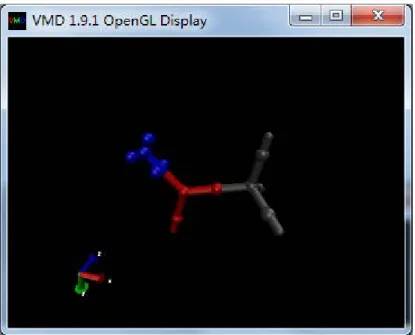
3.3.2 Visualization of Domains . . . . 40
3.4 Special Issues for F12 and High-spin Open-shell Calculations . . . . 41
3.4.1 Perform a F12 Calculation . . . . 41
3.4.2 Perform a High-spin Open-shell Calculation . . . . 42
4 Applications of the Incremental Scheme 45 4.1 Systems from Benchmark Sets . . . . 45
4.2 Water Clusters . . . . 47
4.2.1 Minimum Structure of Water Hexamers . . . . 47
4.2.2 Larger Clusters . . . . 48
4.3 The Rotation Barrier of Biphenyl . . . . 50
4.4 Hydration of Trivalent Lanthanide Ions . . . . 51
4.5 The Relative Stability of Isomers of Double Fullerene Adducts . . . . . 54
4.6 Singlet-triplet Gap of Biphenylcarbene . . . . 58
4.7 VDE of the GFP Chromophore . . . . 60
5 Theory of Labile Capping Bonds and its Applications 63 5.1 Theory of Labile Capping Bonds . . . . 63
5.2 Hydration Kinetics of Trivalent Lanthanide Ions . . . . 68
5.3 Hydration Kinetics of Lanthanide(III)-DOTAM Complexes . . . . 72
6 Summary and Outlook 75 6.1 Summary . . . . 75
6.2 Outlook . . . . 75
Bibliography 77
Abbreviations and Acronyms 95
Acknowledgments 97
CONTENTS v
Erkl¨ arung 99
Curriculum Vitae 100
List of Figures
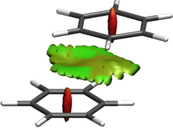
1.2.1 A CMO and Boys-, ER-localized orbital of acetaldehyde. . . . 7 1.8.1 The filled-color map of ELF in the plane of water molecule. . . . 20 1.8.2 The NCI plot of benzene dimer. The red and green surface implies the
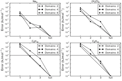
repulsion and weak vdW interaction, respectively. . . . 22 2.1.1 The errors of incremental expansions for four systems versus the trunca-
tion order. The energy is calculated at the CCSD(T)/6-31G(d) level. . . 27 2.2.1 Domain decomposition by KM algorithm. The balls stand for the center
of the LMOs and the balls with identical color belong to the same domain. 28 2.3.1 The procedure of projecting LMOs in B
0onto those in B
X. . . . . 30 2.3.2 Impact of n
dand buffer on the accuracy and efficiency of the incremental
scheme. In the right figure t
Xstands for the wall time of a calculation by method X at the same machine. . . . . 32 2.3.3 Illustration of dual-basis set zero-buffer approximation. Here a HF com-
putation of the molecule is performed with VTZ(p/s) basis set, obtaining the CMOs. After localization the center of the LMOs are computed and represented by balls, and are clustered into domains by KM algorithm.
The balls of identical color belong to the same domain. Then the atoms are clustered by FCKM algorithm to determine the buffer regoin. The last graph illustrates the B0 approximation: to compute the correlation energy of the orange orbital domain, we apply VTZ basis set on the atoms in the orange atom domain, and VTZ(p/s) for the rest of the molecule. 32 2.4.1 The values of the increments for four systems versus the distance. The
energy is calculated at CCSD(T)/6-31G(d) level. . . . 33 3.3.1 Visualization of domains by Vmd . . . . . 41 4.2.1 Some isomers of the water clusters. . . . 49 4.3.1 Biphenyls. The balls stand for the centers of the LMOs and those with
the same color constitute a domain. . . . . 51 4.4.1 Geometries of water clusters (H
2O)
nand lanthanide(III) aqua complexes
Ln(H
2O)
3+n(n = 8, 9). . . . 52 4.4.2 The binding energy errors (unit: kJ mol
−1) with respect to the CCSD(T)
reference for all the considered methods. The errors of method X here are defined as D
CCSD(T)− D
X, where D
Xis the binding energy computed by method X. . . . 54 4.5.1 Molecules investigated for effects of intramolecular dispersion interaction. 56 4.5.2 Geometries and noncovalent interaction visualization. For the surfaces,
red regions mean strong repulsion and green ones mean weak attraction. 58
vii
4.6.1 Left top: Diphenylcarbene. Right top: Diphenylcarbene–methanol com- plex. Bottom: The effect of the methanol molecule suggested by B3LYP- D3 [228] and inc3-db-B0-CCSD(T). . . . 59 4.7.1 Left: The chromophore part of the GFP. Right: The HBDI
−·Gmd
+com-
plex. . . . 60 5.1.1 TZDO/TZDS-aqua-Ln
3+. . . . 63 5.1.2 The lengths, n
BCP’s, and ELF at BCP of the Ln–O bonds in TZDO/TZDS-
aqua-Ln
3+. . . . 64 5.1.3 Colour filled maps of the ELF on two planes of TZDX-aqua-Eu
3+. . . . 66 5.1.4 The lengths, n
BCP’s, and ELF at BCP of the Ln–Cl bonds in LnCl(H
2O)
2+8. 67 5.1.5 The geometries of p- and c-LuCl(H
2O)
2+8. . . . 68 5.2.1 Water exchange rate of lanthanides(III). The figure is adapted from Helm’s
work[247]. . . . 69 5.2.2 Molecular graphs of lanthanide(III) aqua complexes. Red-white licorice:
water molecule; cyan ball: lanthanide(III) ion; yellow ball: bond critical point; green line: bond path; blue line: no physical meaning, just to guide the eye to recognize the coordination polyhedron. There are no bond paths (green lines) connecting lanthanide(III) ions with oxygen atoms since the implementation of PPs for lanthanides depletes the electron density around the nuclei. . . . 70 5.2.3 The lengths, n
BCP’s, and ELF at BCP of the Ln–O bonds in aqua lan-
thanide(III) complexes. . . . . 71 5.2.4 The water exchange mechanism. Other possible steps of association of a
water molecule or rearrangement of a BTP intermediate for nona-aqua lanthanides(III) are omitted for clarity. Circle: water molecule; A: asso- ciation; D: dissociation; R: rearrangement. . . . 72 5.3.1 DOTAM-aqua-Ln
3+. . . . 73 5.3.2 The lengths, n
BCP’s, and ELF at BCP of the Ln–O bonds in DOTAM-
aqua-Ln
3+complexes. . . . 73 5.3.3 The energy difference between the MSAP and MTSAP isomer of DOTAM-
aqua-Ln
3+(A) and bond lengths of Ln-O(prism) in DOTAM-aqua-Ln
3+(B). . . . . 74
List of Tables
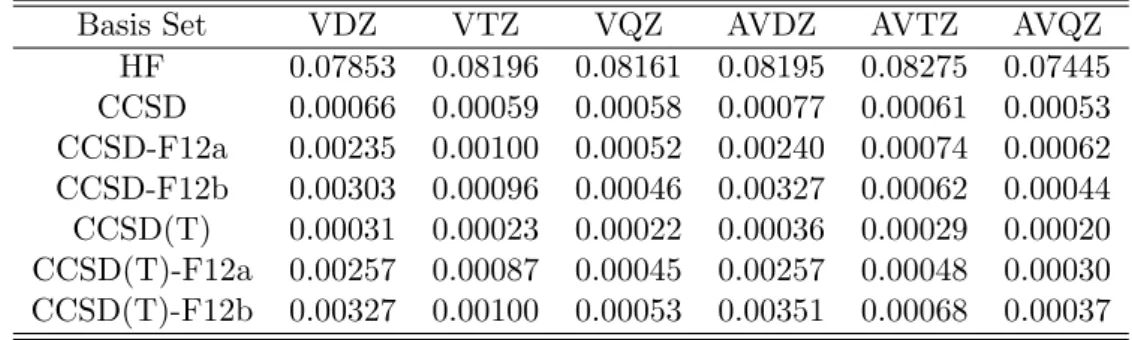
2.3.1 Benchmark of dual-basis set and standard CCSD, CCSD(T), and their F12 variants. . . . 30 4.1.1 Efficiency of inc3-db-B0-F12 methods. All the calculations were per-
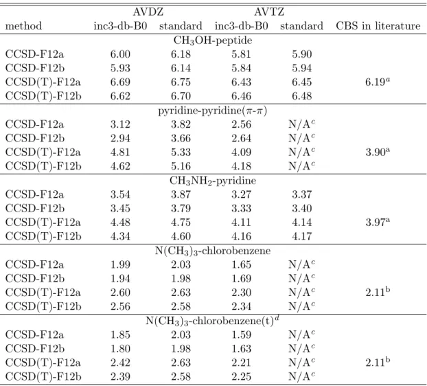
formed with the Intel(R) Xeon(R) E5-4620 CPU cores and 16 GB RAM per core. . . . 46 4.1.2 Interaction energies by inc3-db-B0-F12 methods. Energy unit: kcal mol
−1. 47 4.2.1 Inc3-db-B0-F12 results of water hexamers. The interaction energy is de-
fined as: E
cage− E
prismwith units: kcal mol
−1. All the calculations were performed with the Intel(R) Xeon(R) CPU E7-8837 CPU cores and 8 GB RAM per core. . . . 48 4.2.2 Errors of DLPNO-, OSV- and inc(2/3)-db-B0-CCSD(T)/VDZ methods. 50 4.3.1 Inc3-db-B0-F12 results for the rotation barrier of biphenyl. The inter-
action energy is defined as: E
44◦− E
0◦with unit: kcal mol
−1. All the calculations were performed with the Intel(R) Xeon(R) E5-4620 CPU cores and 16 GB RAM per core. . . . . 51 4.4.1 The RMSDs (unit: kJ mol
−1) of the binding energy errors with respect
to the CCSD(T) reference for all the considered methods. . . . 53 4.4.2 The hydration Gibbs free energies (unit: kJ mol
−1) of lanthanide(III)
aqua complexes. . . . . 55 4.5.1 Energy differences between syn and anti isomers of 2’ to 4’ by ab initio
correlation methods forTPSS-D3/SVP optimized geometries. . . . 56 4.5.2 Energy differences between syn and anti isomers of all molecules consid-
ered by HF and DFT methods for TPSS-D3/SVP optimized geometries. 57 4.6.1 Singlet-triplet gap (unit: kcal mol
−1) of diphenylcarbene and its methanol
complex. . . . 59 4.7.1 VDEs of dHBDI (unit: eV) in gas phase and protein environment. . . . 61 5.1.1 Electronic structure parameters of An
3+complexes. . . . . 66
ix
List of Codes
3.1 Coordinates of CH
3CHO. . . . 36
3.2 An example of node file. . . . 37
3.3 Input file for inc3-db-B0-CCSD(T)/VDZ of CH
3CHO. . . . 37
3.4 Output file of the inc3-db-B0-CCSD(T)/VDZ calculation of CH
3CHO (modified for typesetting). . . . 40
3.5 Tcl script for visualization of domains. . . . 40
3.6 Input file for inc3-db-B0-CCSD(T)-F12/VDZ of CH
3CHO. . . . . 41
3.7 Output file for inc3-db-B0-CCSD(T)-F12/VDZ of CH
3CHO. . . . . 42
3.8 Output file for CCSD(T)-F12/VDZ of CH
3CHO. . . . 42
3.9 Input file for inc3-db-B0-CCSD(T)/VDZ of a triplet state of CH
3CHO. 42 3.10 Output file for inc3-db-B0-CCSD(T)/VDZ of triplet state of CH
3CHO. 43 3.11 Input file for standard dual basis set CCSD(T)/VDZ of triplet state of CH
3CHO, with only the singly occupied orbitals are correlated. . . . 43
3.12 Output file for the Molpro calculation. . . . 44
xi
Chapter 1
Basic Principles of Quantum Chemistry
1.1 Introduction
1.1.1 Molecular Hamiltonian
Quantum chemistry has become a routine tool for scientists to understand a chem- ical problem in a microscopic way. It applies quantum mechanics as well as other modern physics to chemistry to study the movement of electrons in atoms, molecules, clusters, surface, proteins, periodic systems and bulk matters. The starting point to explore the movement of electrons is the molecular Hamiltonian. In this work the Born–Oppenheimer approximation[1] (BO) (fixed nuclei) is assumed, and the nuclei and electrons will be treated as point charges. Thus, in the nonrelativistic case, the Hamil- tonian of a molecule can be written as (in atomic unit):
H ˆ = ˆ T
E+ ˆ V
NE+ ˆ V
EE+ ˆ V
NN≡
N
X
i=1
− 1 2 ∇
2i+
N
X
i=1 K
X
A=1
− Z
Ar
iA+
N
X
i,j=1 i<j
1 r
ij+
K
X
A,B=1 A<B
Z
AZ
Br
AB(1.1.1)
In (1.1.1), N and K stand for the number of electrons and nuclei, respectively; Z
Ais the nuclear charge of the nucleus A; the four terms represent the electron kinetic en- ergy, electron-nucleus attraction energy, electron-electron repulsion energy and nucleus- nucleus repulsion energy, respectively. For ˆ V
NE, we can extract its form for a single electron v
ext(r), which is often called external potential. This term is determined by the molecular framework.
Since ˆ V
EEis a two-electron operator, the molecular quantum mechanics problem becomes a many-body problem, solution of whose equation-of-motion (EOM) is quite nontrivial and becomes the central topic of quantum chemistry.
When a molecule contains heavy atoms (heavier than Fe or Z
A> 26), the relativistic effects cannot be neglected. In this case one can use Dirac–Coulomb Hamiltonian:
H ˆ =
N
X
i=1
cα · p ˆ
i+ βmc
2+ ˆ V
NE+ ˆ V
EE+ ˆ V
NN(1.1.2)
α =
0 σ σ 0
(1.1.3) β =
I
20 0 −I
2(1.1.4)
1
In (1.1.2), c and m are the speed of light and the rest mass of electron, respectively. The three components of σ are Pauli matrices. Note that we do not consider higher-order effects like Breit interation in V
EEyet in (1.1.2).
However this Hamiltonian is quite difficult to work with. Since relativistic effects are most significant in the atomic core region, which is usually chemically inert and thus transferable, one can replace the core part of an atom by an effective one-electron po- tential and only treat the valence electrons explicitly. This is the effective core potential (ECP) approach[2]. It cannot only save the computational cost, but can also take the relativistic and quantum electrodynamic effects, etc. into account in the framework of nonrelativistic theory. In this case the Hamiltonian becomes:
H ˆ = ˆ T
E+ ˆ V
EE+ ˆ V
CV+ ˆ V
CC(1.1.5) where
V ˆ
CV=
NV
X
i=1 K
X
A=1
− Q
Ar
iA+ ∆V
CV,A(r
i)
(1.1.6)
V ˆ
CC=
K
X
A,B=1 A<B
Q
AQ
Br
AB(1.1.7)
From (1.1.5) to (1.1.7), N
Vis the number of valence electrons and Q
Ais the core charge of the nucleus A. ∆V
CV,A(r
i) is the pseudopotential (PP) that constitutes the ECP of nucleus A, with the form[3]:
∆ ˆ V
CV(r) = X
l,m
V
l(r) |lmi hlm| (1.1.8)
In (1.1.8) |lmi is the spherical harmonics function Y
lm(Ω); V
l(r) is the radial part of the PP, which is often written as a linear combination of Gaussian functions multiplied with powers of r[4]:
V
l(r) = X
k
A
lkr
nlkexp −α
lkr
2(1.1.9) In this work we will only consider the Hamiltonian (1.1.1) and (1.1.5).
1.1.2 Wave Function
In quantum mechanics, the motion of an electron is described by its wave function (WFN) ψ (x, t), where x is a collective variable of spatial and spin coordinates x ≡ (r, s) and t is time. For stationary state considered in this work ψ is independent of time. The Copenhagen school interprets the WFN as probability amplitude, that is, the probability density of finding the particle at x at time t is |ψ (x, t)|
2.
An exact molecular electron WFN must satisfy the following conditions:
• ψ is a function of N electrons, or N -representable.
• For bound states, ψ has to be square-integrable (belongs to Hilbert space L
2R
3N), thus normalizable:
hψ| ψi = 1 (1.1.10)
• Since electrons are Fermions, ψ has to be antisymmetric with respect to the per- mutation of two electronic indices:
P
ijψ = −ψ (1.1.11)
1.1. INTRODUCTION 3
• ψ has to satisfy the spin symmetry, being an eigenfunction of the total and pro- jected spin operators:
S ˆ
2ψ = S(S + 1)ψ (1.1.12)
S ˆ
zψ = M ψ (1.1.13)
• ψ has to also satisfy the spatial symmetry, being a basis of one irreducible repre- sentation of the point group to which the molecule belongs.
• Due to the existence of 1/r-like operators in the molecular Hamiltonian, it has to satisfy specific cusp conditions, which will be discussed in Subsection 1.3.2.
• At long range the electron density related to ψ n (r) ≡ N
Z
dsdx
2· · · dx
N|ψ (rs, x
2, · · · , x
N)|
2(1.1.14) decays as[5]:
n (r) → exp
− √ 8Ir
(r → ∞) (1.1.15)
where I is the first ionization potential of the molecule.
Of course this list is far from complete, but a good approximation of the exact WFN should try to satisfy the above conditions as close as possible.
In practice, an approximate WFN is constructed from a set of simple analytical functions, like plane waves or Gaussian functions, which is usually termed as basis set.
1.1.3 Solving the Schr¨ odinger Equation
To obtain the eigenfuntion and eigenvalue of the Hamiltonian, we should solve the time- independent Schr¨ odinger equation (SE)[6]:
Hψ ˆ = Eψ (1.1.16)
Except for a few cases, the SE is impossible to be solved analytically. At this stage the variation principle[7] can be established: the solution of SE is equivalent to the stationary of the energy functional
E [φ] = hφ| H ˆ |φi
hφ| φi (1.1.17)
Proof. Let φ be an exact WFN that satisfies (1.1.16). Assume a variation ˜ φ = φ + δφ then
E [φ + δφ] = hφ| H ˆ |φi + hδφ| H ˆ |φi + hφ| H ˆ |δφi + hδφ| H ˆ |δφi hφ| φi + hδφ| φi + hφ| δφi + hδφ| δφi
= E + hδφ| H ˆ − E |φi + hφ| H ˆ − E |δφi + O δφ
2= E + O δφ
2(1.1.18)
The energy functional proves to be stationary since it does not change at the first-order.
Conversely, if the energy functional is stationary at φ, then according to (1.1.18), for variations ˜ φ = φ + δφ and ˜ φ = φ + iδφ we have
hδφ| H ˆ − E [φ] |φi + hφ| H ˆ − E [φ] |δφi = 0 (1.1.19)
hδφ| H ˆ − E [φ] |φi − hφ| H ˆ − E [φ] |δφi = 0 (1.1.20)
Adding (1.1.19) to (1.1.20) we obtain:
hδφ| H ˆ − E [φ] |φi = 0 (1.1.21)
Since δφ is arbitrary we have (1.1.16). Therefore, the stationary points of the energy functional (1.1.17) and the solutions of SE (1.1.16) have a one-to-one mapping.
In fact, for the exact ground state WFN ψ and a trial WFN φ, we always have
E[ψ] ≤ E[φ] (1.1.22)
In practice the variation principle is always used by constructing a trial WFN with some parameterization ans¨ atze and minimizing the energy functional (1.1.17). One property of parameterization ansatz is the size-extensivity[8]: for a system containing two noninteracting subsystems A and B , the Hamiltonian being
H ˆ
AB= ˆ H
A+ ˆ H
B(1.1.23)
then the energy of the total system is additive and the WFN is multiplicative:
E
AB= E
A+ E
B(1.1.24)
ψ
AB= ψ
A⊗ ψ
B(1.1.25)
A related concept is size-consistency[9]: for a system containing two subsystems A and B, when A and B are very far apart, the energy is additive:
E
AB= E
A+ E
B(1.1.26)
The size-extensivity and consistency ensure that the accuracy of energies of large and small systems can be consistent, otherwise the error for the larger system tends to be larger, leading to a relative energy of bad quality.
1.2 Single-particle Approximation
1.2.1 Hartree–Fock Method
The first step of approximating an exact N-electron molecular WFN is assuming it be the product of N one-electron WFNs:
ψ
Hartreex
N=
N
Y
i=1
φ
i(x
i) (1.2.1)
This is called Hartree product [10, 11]. The φ
idescribes the motion of electron i thus it is called molecular orbital (MO). To make it satisfy the antisymmetry requirement (1.1.11), an antisymmtrizer A can be applied, leading to a Slater determinant (SD)[12]:
ψ
SDx
N= |φ
1· · · φ
Ni ≡ 1
√ N !
φ
1(x
1) · · · φ
1(x
N) .. . . .. .. . φ
N(x
1) · · · φ
N(x
N)
(1.2.2)
A single SD can be used as the trial WFN, which is the Hartree–Fock (HF) WFN[13]:
|HFi =
N
Y
i=1
a
†i|vaci (1.2.3)
1.2. SINGLE-PARTICLE APPROXIMATION 5 Now we can optimize the energy functional (1.1.17) with respect to the MOs. To ensure |HFi is normalized, we can restrict that the MOs are orthonormal:
hφ
i| φ
ji = δ
ij(1.2.4)
In this case we have to optimize the Lagrangian L [{φ}] = hHF| H ˆ |HFi −
N
X
i,j=1
ij(hφ
i| φ
ji − δ
ij) (1.2.5) rather than the energy functional directly. Using the Hamiltonian (1.1.1)
E
HF≡ hHF| H ˆ |HFi =
N
X
i=1
hφ
i| ˆ h |φ
ii + 1 2
N
X
i,j=1
(hφ
iφ
j| φ
iφ
ji − hφ
iφ
j| φ
jφ
ii) + E
NN(1.2.6) where E
NNis the nucleus-nucleus repulsion energy. Now we can compute the variation of (1.2.5):
δL [{φ}] =
N
X
i=1
hδφ
i| h ˆ |φ
ii +
N
X
i,j=1
(hδφ
iφ
j| φ
iφ
ji − hδφ
iφ
j| φ
jφ
ii)
−
N
X
i,j=1
ijhδφ
i| φ
ji + c.c.
=
N
X
i=1
Z
dx
1δφ
∗i(x
1)
ˆ hφ
i+
N
X
j=1
Z
dx
2φ
∗j(x
2) 1 r
12φ
j(x
2)
φ
i(x
1)
−
N
X
j=1
Z
dx
2φ
∗j(x
2) 1 r
12φ
i(x
2)
φ
j(x
1) −
N
X
j=1
ijφ
j(x
1)
+ c.c.
≡
N
X
i=1
Z
dx
1δφ
∗i(x
1)
ˆ h (1) + ˆ J (1) − K ˆ (1)
φ
i(x
1) −
N
X
j=1
ijφ
j(x
1)
+ c.c.
≡
N
X
i=1
Z
dx
1δφ
∗i(x
1)
f ˆ (1) φ
i(x
1) −
N
X
j=1
ijφ
j(x
1)
+ c.c.
(1.2.7) In (1.2.7), ˆ J and ˆ K are the Coulomb and exchange operator, respectively. ˆ f is called Fock operator, which is the effective one-electron operator that determines the optimized MOs. Note that Lagrangian (1.2.5) has to be real thus by L = L
∗we can prove that
∗ij=
ji, i.e. is an Hermite matrix, being diagonalizable. Therefore we can find a unitary transformation U of the MOs {φ}
φ ˜
i=
N
X
j=1
φ
jU
ji(1.2.8)
φ
i=
N
X
j=1
φ ˜
jU
ij∗(1.2.9)
that diagonalizes
N
X
k,l=1
U
ki∗klU
lj= δ
iji(1.2.10) Substitute (1.2.9) into (1.2.7), and use (1.2.10), let δL = 0. Note that {δφ} is arbitrary, we obtain the canonical Hartree–Fock equation (tildes removed):
f φ ˆ
i=
iφ
i(i = 1, · · · , N ) (1.2.11) Since ˆ f depends on {φ}, (1.2.11) has to be solved iteratively. Thus it is also called self-consistent field (SCF) method. Except for atoms and diatomic molecules, (1.2.11) usually cannot be solved numerically. To transform it into an algebraic problem, given a basis set {χ} is used (also known as atomic orbitals (AOs)) that expands MOs:
φ
p= X
µ
χ
µC
µp(1.2.12)
Note that we use subindex p instead of i, implying that φ
pis not necessarily an occupied orbital. We will always use i, j, k, l to stand for occupied orbitals, a, b, c, d for unoccupied (virtual) orbitals and p, q, r, s for arbitrary orbitals.
By substituting (1.2.12) into (1.2.11) and taking the inner product with χ
∗, we obtain the Roothaan–Hall equation[14, 15]:
FC = SC (1.2.13)
F
µν= hµ| ˆ h |νi + X
ρτ
D
ρτ(hµρ| ντ i − hµρ| τ ν i) (1.2.14) D
µν= X
i
C
µi∗C
νi(1.2.15)
S
µν= hµ| νi (1.2.16)
Here D is the density matrix in AO basis. This equation is much easier to solve. The obtained orbitals from (1.2.14) are called canonical MOs (CMOs).
1.2.2 Molecular Orbitals
The Hartree–Fock method is not only the cornerstone of advanced ab initio methods, but also has its own value. For the Hilbert space spanned by a basis set {χ}, the MO basis can be transformed into another one by a unitary transformation (preserving their inner products), and the WFN constituted by these two bases can be related as:
ψ ˜
E
= exp (−ˆ κ) |ψi ≡ exp − X
pq
κ
pqa
†pa
q!
|ψi (1.2.17)
Now we look at the HF energy with transformed orbitals:
E (κ) = hHF| exp (ˆ κ) ˆ H exp (−ˆ κ) |HFi
= E
HF+ hHF| h ˆ κ, H ˆ i
|HFi + · · ·
= E
HF+ X
pq
hHF| h
a
†pa
q, H ˆ i
|HFi κ
pq+ · · ·
(1.2.18)
If the energy E is already stationary, we will have 0 = ∂E (κ)
κ
pqκ=0
= hHF| h
a
†pa
q, H ˆ i
|HFi (1.2.19)
1.2. SINGLE-PARTICLE APPROXIMATION 7 For nonredundant rotations, e.g. pq = ai, we have
hHF| h a
†aa
i, H ˆ
i
|HFi = a
i
H ˆ |HFi = f
ai= 0 (1.2.20) which is known as Brillouin theorem[13].
For redundant rotations, i.e. p, q are both occupied or unoccupied orbitals, ∂E (κ) /∂κ
pqand hence higher-order terms involving these κ
pqwill always be zero due to the Pauli’s principle, indicating that orbital rotations within occupied or virtual space do not change the WFN and its energy. Thus it is possible to transform the occupied MOs obtained from (1.2.14) into a chemically more meaningful set without changing the WFN and energy.
Since CMOs are orthogonal and symmetry-adapted to the molecular point group, they are often very delocalized, thus one can rotate them to obtain localized MOs (LMO) with specific criteria. Two typical choices are:
• Boys criterion[16], which aims at minimizing the spatial extent:
L
Boys[{φ}] = max :
occ
X
i
hφ
iφ
i|(r
1− r
2)| φ
iφ
ii (1.2.21)
• Edmiston–Ruedenberg criterion (ER)[17], which aims at maximizing the self-repulsion energy:
L
ER[{φ}] = max :
occ
X
i
hφ
iφ
i| φ
iφ
ii (1.2.22) One advantage of ER over Boys criterion is that the former can preserve the σ-π symmetry of the MOs[18], but both have a very good localization effect. An example of CMO and LMO can be seen in Figure 1.2.1.
CMO Boys ER
Figure 1.2.1: A CMO and Boys-, ER-localized orbital of acetaldehyde.
Localization is usually performed in an iterative way[17]. In each iteration, every two orbitals are rotated with an optimized angle that satisfies (1.2.21) or (1.2.22):
φ ˜
iφ ˜
j=
cos θ sin θ
− sin θ cos θ
φ
iφ
j(1.2.23)
tan 4θ = − A
ijB
ij(1.2.24)
A
ij= hφ
iφ
i| Γ ˆ |φ
iφ
ji − hφ
jφ
j| Γ ˆ |φ
iφ
ji (1.2.25) B
ij= hφ
iφ
j| Γ ˆ |φ
iφ
ji − 1
4
hφ
iφ
i| Γ ˆ |φ
iφ
ii + hφ
jφ
j| Γ ˆ |φ
jφ
ji − 2 hφ
iφ
i| Γ ˆ |φ
jφ
ji
(1.2.26)
where ˆ Γ is the operator related to (1.2.21) or (1.2.22). The iteration continues until convergence is reached.
This method is effective for occupied orbitals of most molecules. For virtual or- bitals or very delocalized systems (like graphene), this method can be very difficult to converge[19]. In this case one can explicitly optimize the orbital rotation parameters in (1.2.17) to force convergence[20].
1.3 Electron Correlation
1.3.1 Fermi and Coulomb Correlation
With a molecular WFN, we can define the one-electron and pair probability density:
P (r) ≡ Z
ds
1dx
2· · · dx
N|ψ (rs
1, x
2, · · · , x
N)|
2(1.3.1) P r, r
0≡ Z
ds
1ds
2dx
3· · · dx
Nψ rs
1, r
0s
2, x
3, · · · , x
N2
(1.3.2)
as well as a conditional probability density : P r|r
0≡ P (r, r
0)
P (r
0) (1.3.3)
For two electrons 1 and 2, their motion is said to be uncorrelated if
P (r
1|r
2) = P (r
1) (1.3.4)
Take the
3Σ
+ustate of a two-electron molecule H
2as an example. Assuming it contains only two orbitals: σ
gand σ
u, we can see that for a Hartree product WFN (1.2.1):
P (r
1|r
2) = P (r
1) = |σ
g(r
1)|
2(1.3.5) the two electrons are uncorrelated.
For a SD WFN |σ
gσ
ui, we have P (r
1) = 1
2
|σ
g(r
1)|
2+ |σ
u(r
1)|
2(1.3.6) P (r
1, r
2) = 1
2
|σ
g(r
1)|
2|σ
u(r
2)|
2+ |σ
u(r
1)|
2|σ
g(r
2)|
2− σ
u∗(r
1) σ
g(r
1) σ
g∗(r
2) σ
u(r
2) (1.3.7) Therefore there is electron correlation generated from the antisymmetry requirement of SD, known as Fermi correlation. In this case, the Fermi correlation lowers the probability density of finding an electron at r
1and an electron at r
2, thus it is called Fermi hole.
For the
1Σ
+ustate, the Fermi correlation increases this probability, thus it is a Fermi heap.
Due to the two-electron Coulomb interactions, a single SD WFN (1.2.2) is far from being accurate although it is a good zero-order approximation. An exact WFN should contain an infinite number of SDs, written as
|ψi = |HFi + |excited SDsi (1.3.8)
The extra terms also introduce electron correlation, known as Coulomb correlation.
Recovering Coulomb correlation is critical to get a chemically useful WFN and energy,
however it is also quite difficult.
1.3. ELECTRON CORRELATION 9 1.3.2 Cusp Conditions
The 1/r-like operators in Hamiltonians (1.1.1), (1.1.2) and (1.1.5) are singular at r = 0.
To keep the eigenvalue of ˆ H or the energy finite, the kinetic term, i.e. ∇
2ψ-like term, should also be singular. This implies at r = 0 the ∇ψ might be discontinuous. In fact, Kato stated the famous cusp condition[21] in 1957 that for a nonrelativistic Hamiltonian (1.1.1), the first-order derivative of an exact eigenfunction must be discontinuous at the singular points of the Coulomb operators.
This can be understood by analyzing the behavior of SE at the neighborhood of a point where two particles of charge q
1and q
2meet, their reduced mass being µ. In this region we can expand the WFN:
ψ (r) = X
lm
X
k=0
r
l+kf
lmkY
lm(Ω) (1.3.9) and only the Hamiltonian involving the two particles becomes significant. Then:
Eψ (r) =
− 1
2µ ∇
2+ q
1q
2r
ψ (r)
= − 1 2µ
1 r
∂
2∂r
2r + 1 2µ
L ˆ
2r
2+ q
1q
2r
! X
lm
X
k=0
r
l+kf
lmkY
lm(Ω)
(1.3.10)
After rearrangement and taking an inner product with Y
lm∗(Ω):
l + 1
µ f
lm1− q
1q
2f
lm0r
l−1+ X
k=0
Ef
lmk− q
1q
2f
lmk+1+ 1
2µ (k + 2) (k + 2l + 3) f
lmk+2r
l+k= 0
(1.3.11)
Since r is arbitrary, we have
f
lm1= µq
1q
2l + 1 f
lm0(1.3.12)
Also note that
f
lmk= 1 (l + k)!
^ ∂
l+kψ
∂r
l+k lmr=0
(1.3.13) where ( ) e
lmmeans projection of angular coordinates onto |lmi.
For two electrons, µ = 1/2 and q
1= q
2= −1. If the WFN is totally symmetric, then (1.3.12) holds for l = 0:
∂ψ
∂r
r=0= 1
2 ψ (r = 0) (1.3.14)
or
ψ (r) =
1 + 1 2 r
ψ (r = 0) + O r
2(1.3.15) (1.3.14) or (1.3.15) are often called s-wave coalescence condition or simply electron cusp condition. For triplet symmetry, l = 1, we have p-wave coalescence condition:
ψ (r) =
1 + 1 4 r
r · ∇ψ (r = 0) + O r
3(1.3.16) For WFN of other symmetries or relativistic Hamiltonians, different coalescence conditions are required[22, 23].
The cusp condition poses a tough requirement on the basis set by which a WFN is
constructed. Since an exact WFN contains odd powers of the inter-electron distance,
basis functions of very high angular momentum and a large number of many-particle
basis functions are required to model this behavior.
1.3.3 Correlation Energy
According to L¨ owdin[24], the correlation energy is defined as the difference between the exact nonrelativistic energy and the HF energy (both computed in a complete basis set (CBS)):
E
corr= E − E
HF(1.3.17)
In practice, quantum chemistry is often used to compute relative energies, and the magnitude of correlation energy is often the largest one. For a typical relative electronic energy of a molecule containing only light elements, the correlation part usually amounts to 1%–2%. Other parts, like relativistic effect and diagonal BO correction, are less than 0.2%. Thus, a large amount of effort has been invested to efficiently obtain accurate correlation energies.
1.4 Many-body Approaches
1.4.1 Full Configuration Interaction Expansion Linear Parameterization Ansatz
The HF WFN (1.2.6), i.e. a single SD (1.2.2), is not an exact solution of the SE (1.1.16). To approach the exact WFN more many-particle basis functions are needed.
In the solution of Roothaan–Hall equation (1.2.14), we obtain not only occupied orbitals O but also virtual (unoccupied) orbitals V . The many-particle basis {|µi} can then be constructed systematically by excitation of 1, 2, · · · , N electrons from the HF WFN:
a i
≡ a
†aa
i|HFi = n a
†aa
io
|HFi (1.4.1)
ab ij
≡ a
†aa
†ba
ja
i|HFi = n
a
†aa
ia
†ba
jo
|HFi (1.4.2)
where {} denotes the normal order relative to the Fermi vacuum, i.e. HF WFN. The exact WFN can be approximated by the linear combination of all the SDs:
|FCIi = |HFi + X
ai
c
ain
a
†aa
io
|HFi + 1 4
X
abij
c
abijn
a
†aa
ia
†ba
jo
|HFi + · · ·
≡
1 + ˆ C
1+ ˆ C
2+ · · ·
|HFi
(1.4.3)
This is the full configuration interaction (FCI) WFN, where a linear parameterization ansatz is implemented. In practice a truncated version of (1.4.3) has to be used. However a truncated CI WFN suffers from lacking size-extensivity. This can be seen from two noninteracting systems A and B described by CI doubles (only doublet excitations are considered, CID), the direct product of |CIDi
Aand |CIDi
Bcontains quadruple excitations, which is not taken in account in |CIDi
AB.
Determination of parameters in the CI WFN is a seemingly trivial task. Assuming the WFN is real:
|CIi = X
µ
c
µ|µi (1.4.4)
E (c) = hCI| H ˆ |CIi hCI |CIi =
P
µν
c
µc
νH
µνP
µ
c
2µ(1.4.5)
g
µ(c) ≡ ∂E
∂c
µg = 2 (H − E (c) I) c
c
Tc (1.4.6)
1.4. MANY-BODY APPROACHES 11
G
µν(c) ≡ ∂
2E
∂c
µ∂c
νG = 2
H − E (c) I − g (c) c
T− cg (c)
Tc
Tc (1.4.7)
Using g = 0, we can obtain the scalar equation :
Hc = Ec (1.4.8)
Davidson Iteration
Equation (1.4.8) can be solved by, say Jacobi–Givens iteration. However, for large systems, it is sometimes even not possible to store the whole H in memory, thus one is always trying to avoid the explicit construction of H. If the solving procedure only involves Hc then the avoidance is possible. An additional advantage is that we need not to calculate all the eigenvalues but only some interested ones, like ground and lowest excited states.
A popular method is the Davidson iteration[25]. We need a reference H
0whose eigenvector c
0and eigenvalue E
0are easy to compute (usually the diagonal part of H).
Consider the required solution c = c
0+ d, and a Taylor expansion of energy (1.4.5) at c
0:
E (c
0+ d) = E
0+ d
Tg (c
0) + 1
2 d
TG (c
0) d + · · · (1.4.9) Truncate (1.4.9) at second-order, and optimized E with d, we obtain
d = −G (c
0)
−1g (c
0)
= −
H − E
0I − g (c
0) c
T0− c
0g (c
0)
T−1(H − E
0I) c
0(1.4.10) If c
0is a good approximation, then g (c
0) ≈ 0, and we replace H in the inverse by H
0, we obtain the final iteration formula:
d = − (H
0− E
0I)
−1(H − E
0I) c
0(1.4.11) This is much more efficient then the diagonalization of H (1.4.8). Note that in (1.4.11), the convergence slows down if H
0and H are close to each other. In fact:
d → −c
0as H
0→ H (1.4.12)
Convergence to the Exact Solution of the Schr¨ odinger Equation
Finally we want to give some results from functional analysis. If the (one-particle) basis set is complete in the Hilbert space L
2R
3, then the set of all possible SDs forms a complete many-particle basis in the Hilbert space L
2R
3N. Therefore a complete basis set can in principle be used to obtain convergence towards the exact WFN to any accuracy in the norm p
hf |f i (i.e., not pointwisely convergent). However, to ensure the solutions of FCI (1.4.8) converge to the exact WFNs, it has been proved[26, 27] that the basis set has to be complete in the first Sobolev space (the space of functions where the function and its first-order derivative are square-integrable). This is obviously a consequence of the kinetic operator ˆ T
e.
1.4.2 Perturbation Theory Formal Theory
Since HF WFN is an eigenfunction of the effective Hamiltonian H ˆ
0=
N
X
i=1
f ˆ
i(1.4.13)
with eigenvalue E
0(0)= P
Ni=1
i, then it is also possible to improve HF (|HFi ≡ |0i) using {|µi} by perturbation expansion of an flucuation potential:
W ˆ ≡ H ˆ − H ˆ
0(1.4.14)
Here we give a general derivation of perturbation theory[28]. For exact WFN ψ and its SE, we project it onto the HF WFN:
h0| H ˆ
0|ψi + h0| W ˆ |ψi = E h0|ψi (1.4.15) at this step it is convenient to assume intermediate normalization: h0|ψi = 1 so that
∆E = h0| W ˆ |ψi (1.4.16)
where ∆E = E − E
0(0). This is the energy expression.
To derive the WFN expression, we introduce a projection operator
P ˆ = |0i h0| (1.4.17)
Q ˆ = X
µ
0
|µi hµ| (1.4.18)
where “
0” means that the summation does not include |0i. Then we the rearrange SE, and add E
0(0)to both sides, and apply ˆ Q:
Q ˆ
E
0(0)− H ˆ
0ψ = ˆ Q
E
0(0)+ ˆ W − E
ψ (1.4.19)
Note that ˆ Q commutes with ˆ H
0and is idempotent, the left operator can completely work in Q-space:
Q ˆ
E
0(0)− H ˆ
0Qψ ˆ = ˆ Q
E
0(0)+ ˆ W − E
ψ (1.4.20)
Due to the nature of ˆ Q, the inverse operator in the Q-space (means ˆ A B ˆ = ˆ B A ˆ = ˆ Q) of ˆ Q
E
0(0)− H ˆ
0Q ˆ exists, which is written as
R ˆ
0≡ Q ˆ E
0(0)− H ˆ
0(1.4.21) this is the resolvent of ˆ H
0. Apply it to (1.4.20):
Qψ ˆ = ˆ R
0E
0(0)+ ˆ W − E
ψ (1.4.22)
and using ψ = ˆ Qψ + |0i
ψ = |0i + ˆ R
0E
0(0)+ ˆ W − E
ψ (1.4.23)
This expression can be used in a Picard iteration way:
|ψi =
+∞
X
m=0
R ˆ
0E
0(0)+ ˆ W − E
m|0i (1.4.24)
Using (1.4.16), we have Rayleigh–Schr¨ odinger perturbation theory (RSPT) formulae:
∆E =
∞
X
m=0
h0| W ˆ R ˆ
0W ˆ − ∆E
m|0i (1.4.25)
1.4. MANY-BODY APPROACHES 13
|ψi =
∞
X
m=0
R ˆ
0W ˆ − ∆E
m|0i (1.4.26)
For (1.4.25), we again use Picard iteration to get an explicit expression of ∆E.
∆E = h0| W ˆ |0i + h0| W ˆ R ˆ
0W ˆ |0i + h0| W ˆ R ˆ
0W ˆ − h0| W ˆ |0i
R ˆ
0W ˆ |0i + · · ·
≡ E
0(1)+ E
0(2)+ E
0(3)+ · · ·
(1.4.27)
In fact,
E
0(1)= − 1 2
X
ij
hij| |iji (1.4.28)
Adding E
0(1)to E
0(0)one obtains E
HF. Define:
V ˆ ≡ W ˆ − h0| W ˆ |0i (1.4.29)
and note that for any constants c, ˆ R
0c |0i = 0, so
E
corr= h0| V ˆ R ˆ
0V ˆ |0i + h0| V ˆ R ˆ
0V ˆ R ˆ
0V ˆ |0i + · · · (1.4.30) Linked-diagram Theorem
Linked-diagram theorem[28, 29] states that, only terms of linked-diagram can contribute to the energy and WFN, i.e.
|ψi =
+∞
X
m=0
R ˆ
0V ˆ
m|0i
L(1.4.31)
E
corr=
+∞
X
m=1
h0| V ˆ
R ˆ
0V ˆ
m|0i
L(1.4.32)
As a trivial example, the second-order energy E
0(2)is E
(2)0= h0| V ˆ R ˆ
0V ˆ |0i
=
= 1 4
X
abij
hij | |abi hab| |iji
abij(1.4.33)
where
abij≡
a+
b−
i−
j. When adding it to the HF energy, the obtained one is called second-order Møller–Plesset (MP2) energy.
A nontrivial example is the fourth-order energy E
0(4):
E
0(4)= h0| V ˆ R ˆ
0V ˆ R ˆ
0V ˆ R ˆ
0V ˆ |0i − h0| V ˆ R ˆ
0R ˆ
0V ˆ |0i h0| V ˆ R ˆ
0V ˆ |0i (1.4.34) The two terms in (1.4.34) are called principal and renormalization terms, respectively.
In fact, the unlinked diagrams in the first term cancel with the renormalization term.
There are only two unlinked diagrams which are +
= 1 16
X
abcd ijkl
hij| |abi hab| |ij i hcd| |kli hkl| |cdi
abijabcdijklcdkl+ 1 16
X
abcdijkl
hij| |abi hab| |ij i hcd| |kli hkl| |cdi
abijabcdijklabij=
1 4
X
abij
hij| |abi hab| |iji
abij2
1 4
X
abij
hij | |abi hab| |iji
abij
= × = h0| V ˆ R ˆ
0R ˆ
0V ˆ |0i h0| V ˆ R ˆ
0V ˆ |0i
(1.4.35)
which confirms the linked-diagram theorem.
1.4.3 Coupled-cluster Ansatz Coupled-cluster Equation
A more advanced parameterization ansatz can be constructed from some physical con- sideration. Define m-body excitation operator:
T ˆ
m≡ 1 (m!)
2X
a1a2···am i1i2···im
t
ai11ia22···i···ammn
a
†a1a
i1a
†a2a
i2· · · a
†ama
imo
(1.4.36)
Here we use t as parameters, different from c in (1.4.3). In a molecule, ˆ T
mdescribes that m electrons being excited simultaneously (connected cluster ) from Fermi vacuum.
In a FCI expansion, ˆ T
malso contribute to the case of two independent (unconnected cluster ) m-excitation as
12T ˆ
m2, three independent m-excitation as
3!1T ˆ
m3, etc. Thus its whole contribution is:
1 + ˆ T
m+ 1 2
T ˆ
m2+ 1 3!
T ˆ
m3+ · · · = e
Tˆm(1.4.37) Note that as ˆ T
mand ˆ T
nare commutative, the FCI expansion can be written as a product over all levels of excitation, also known as coupled-cluster (CC) expansion[30]:
|CCi = Y
m
e
Tˆm|HFi = exp X
m
T ˆ
m!
|HFi ≡ e
Tˆ|HFi (1.4.38) where ˆ T is called cluster operator.
CC is one of the most successful ab initio quantum chemistry methods. Due to the exponential parameterization ansatz, even a truncated version can implicitly describe higher-order excitations via unconnected terms, thus its energy can be very accurate. In fact, it is these unconnected terms that make CC an size-extensive method. A variation determination of CC parameters is rather difficult due to the complexity of the equations.
Thus, one can project the SE onto HF and excited SD states to obtain the linked CC equation :
E
CC= hHF| e
−TˆHe ˆ
Tˆ|HFi (1.4.39)
1.4. MANY-BODY APPROACHES 15 0 = hµ| e
−TˆHe ˆ
Tˆ|HFi (1.4.40) When the cluster operator is truncated at the second-order, we obtain CC singles and doubles (CCSD) equations[31]. An explicit expression is rather awkward to derive al- gebraically. However, diagrammatic notations can facilitate the procedure significantly and elegantly. The CC energy:
E
CC= E
HF+ hHF| e
−TˆH ˆ
Ne
Tˆ|HFi
= E
HF+ hHF| H ˆ
NT ˆ
1+ ˆ T
2+ 1 2
T ˆ
12|HFi
C= E
HF+ + +
= E
HF+ X
ai
f
ait
ai+ 1 4
X
abij
hij| |abi t
abij+ 1 2
X
abij
hij | |abi t
ait
bj(1.4.41)
where ˆ H
Nis the normal-ordered Hamiltonian, “C” means that only terms involving contractions of ˆ H
Nand all ˆ T on the right are considered. This leads to the fact that only linked diagrams are involved. Of course for a HF reference all f
aiwill be zero.
For the amplitude equation (1.4.40) more diagrams are required but the procedure is similar. These equations are solved iteratively.
Perturbative Treatment of Coupled-cluster Ansatz
For chemical accuracy, three-body cluster operator ˆ T
3must be taken into account, but the extremely high computational cost forbids this for even some small molecules. How- ever, it is found that these three-body cluster amplitudes can be treated using the converged single and double amplitudes in a perturbative way without too much loss of accuracy, leading to the CCSD(T) method[32].
It is argued that the performance of CCSD(T) relies on an error cancelation: the perturbative treatment overestimates the energy associated with triples, and canceled by the neglect of quadruples In fact, the accuracy of CCSD(T) is comparable with that of all-electron, relativistic CCSDT(Q)[33]. Thus, CCSD(T)/CBS is often used as benchmark reference and recognized as the “gold standard” of quantum chemistry.
1.4.4 Explicit Correlation Methods
The basis set used in practice is often incomplete, leading to the basis set incompleteness error (BSIE). In fact, in order to reproduce the cusp condition (1.3.15), basis functions of very high angular momenta up to f, g, · · · are needed. To reduce the basis set size and accelerate the basis set convergence, one can explicitly introduce the inter-electron distance r
12to the WFN parameterization ansatz in a (1.3.15)-like way[23, 34].
A popular way is to introduce r
12into the CCSD formula, obtaining the simplified CCSD-F12 theory[35, 36]. Its WFN is:
|ψi = exp
T ˆ
1+ ˆ T
2+ ˆ T
20|HFi (1.4.42)
T ˆ
20= 1 4
X
αβij