Product Market Deregulation and the U.S. Employment Miracle

IHS Economics Series Working Paper 223

May 2008

Product Market Deregulation and the U.S. Employment Miracle

Monique Ebell

Christian Haefke

Impressum Author(s):

Monique Ebell, Christian Haefke Title:

Product Market Deregulation and the U.S. Employment Miracle ISSN: Unspecified

2008 Institut für Höhere Studien - Institute for Advanced Studies (IHS) Josefstädter Straße 39, A-1080 Wien

E-Mail: o ce@ihs.ac.atffi Web: ww w .ihs.ac. a t

All IHS Working Papers are available online: http://irihs. ihs. ac.at/view/ihs_series/

This paper is available for download without charge at:

https://irihs.ihs.ac.at/id/eprint/1839/

Product Market Deregulation and the U.S. Employment

Miracle

Monique Ebell, Christian Haefke

223

Reihe Ökonomie

Economics Series

223 Reihe Ökonomie Economics Series

Product Market Deregulation and the U.S. Employment

Miracle

Monique Ebell, Christian Haefke

May 2008

Contact:

Monique Ebell

Department of Economics and Business Studies Humboldt University of Berlin

and

Centre for Economic Performance London School of Economics and Political Science

email: M.Ebell@lse.ac.uk

Christian Haefke

Department of Economics and Finance Institute for Advanced Studies Stumpergasse 56

1060 Vienna, Austria : +43/1/599 91-181

email: christian.haefke@ihs.ac.at and

Instituto de Análisis Económico, CSIC

Founded in 1963 by two prominent Austrians living in exile – the sociologist Paul F. Lazarsfeld and the economist Oskar Morgenstern – with the financial support from the Ford Foundation, the Austrian Federal Ministry of Education and the City of Vienna, the Institute for Advanced Studies (IHS) is the first institution for postgraduate education and research in economics and the social sciences in Austria.

The Economics Series presents research done at the Department of Economics and Finance and aims to share “work in progress” in a timely way before formal publication. As usual, authors bear full responsibility for the content of their contributions.

Das Institut für Höhere Studien (IHS) wurde im Jahr 1963 von zwei prominenten Exilösterreichern – dem Soziologen Paul F. Lazarsfeld und dem Ökonomen Oskar Morgenstern – mit Hilfe der Ford- Stiftung, des Österreichischen Bundesministeriums für Unterricht und der Stadt Wien gegründet und ist somit die erste nachuniversitäre Lehr- und Forschungsstätte für die Sozial- und Wirtschafts- wissenschaften in Österreich. Die Reihe Ökonomie bietet Einblick in die Forschungsarbeit der Abteilung für Ökonomie und Finanzwirtschaft und verfolgt das Ziel, abteilungsinterne Diskussionsbeiträge einer breiteren fachinternen Öffentlichkeit zugänglich zu machen. Die inhaltliche

Abstract

We consider the dynamic relationship between product market entry regulation and equilibrium unemployment. The main theoretical contribution is combining a job matching model with monopolistic competition in the goods market and individual bargaining. We calibrate the model to US data and perform a policy experiment to assess whether the decrease in trend unemployment during the 1980’s and 1990’s could be directly attributed to product market deregulation. Under a traditional calibration, our results suggest that a decrease of less than two-tenths of a percentage point of unemployment rates can be attributed to product market deregulation, a surprisingly small amount. Under a small surplus calibration, however, product market deregulation can account for the entire decline in US trend unemployment over the 1980’s and 1990’s.

Keywords

Product market competition, barriers to entry, wage bargaining

JEL Classifications

E24, J63, L16, O00

Comments

We thank Philippe Bacchetta, Olivier Blanchard, Jan Boone, Michael Burda, Antonio Cabrales, Jordi Galí, Adriana Kugler, Etienne Lehmann, Pietro Peretto, Chris Pissarides, Julien Prat, Michael Reiter, Albrecht Ritschl, Roberto Samaniego, Eric Smith, Chris Telmer, Harald Uhlig, and Fabrizio Zilibotti for helpful comments and discussions. Two anonymous referees and an associate editor provided valuable suggestions that substantially improved this paper. We also thank seminar audiences at Cambridge, Duke, the European Central Bank, Humboldt, IZA, Tilburg, UPF, and Universitat Autonoma de Barcelona, as well as the participants of the 2003 European Summer Symposium in Macroeconomics, 2003 North American Winter Meetings of the Econometric Society, the CEPR DAEUP meeting in Berlin and the 2003 SED meetings for helpful comments. All remaining errors are

Contents

1 Introduction 1

2 The Basic Model 3

2.1 Households... 4

2.1.1 Monopolistic Competition in the Goods Market ... 4

2.1.2 Search and Matching in the Labor Market... 4

2.2 Multiple-worker Firms ... 5

2.3 Wage Bargaining ... 6

2.3.1 Individual Bargaining Solution ... 7

2.3.2 Labor demand and the wage curve ... 8

3 Equilibrium 8

3.2 Hiring Externality... 9

3.3 Short Run General Equilibrium ... 10

3.3.1 Comparative Statics I: Varying Competition... 11

3.3.2 Comparative Statics II: Varying Parameters ... 12

3.4 Long-run General Equilibrium... 13

4 Quantitative Results 14

4.1.1 Traditional vs Small Surplus Calibration ... 15

4.1.2 Entry Costs ... 16

4.1.3 Baseline 1998 Calibrations ... 16

4.2 Product Market Deregulation and the Labor Market... 17

4.3 Interactions ... 18

4.3.1 Labor taxation ... 18

4.3.2 Worker’s bargaining power ... 18

4.3.3 Matching efficiency ... 19

4.4 Quantifying Overhiring ... 19

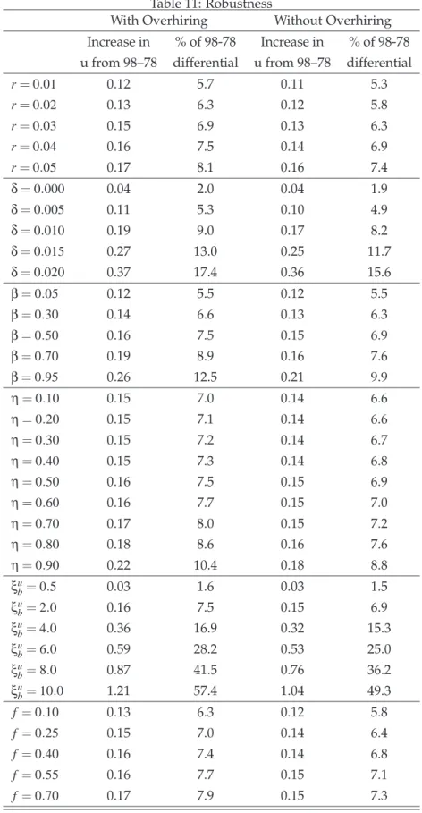
4.5 Robustness ... 20

5 Conclusions 20

Appendix A Proofs and Derivations 25

Appendix B Tables 29

Appendix C Figures 35

1 Introduction

This paper studies the impact of product market deregulation on labor markets, with spe- cial emphasis on the Carter/Reagan deregulation of the late 1970’s and early 1980’s.

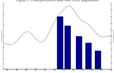
There has been quite some interest recently in the impact of product market institutions on labor markets. However, the focus of this literature has been to use differences in US and European product market regulation to try to explain the divergent performance of US and European labor markets over the 1980’s and 1990’s. One obstacle faced by this literature is that the presence of a multitude of rigidities (and attempts at reform) in European labor markets makes it difficult to disentangle the roles of product and labor market institutions in accounting for high European unemployment rates. In contrast, the US labor market is both highly flexible and its institutions were more stable during the period of interest (Figure2). This allows us to focus only on changes in product market regulation, while holding labor market institutions constant.

Consider the graph of HP-trend unemployment rates¹in Figure1. US unemployment rates began trending downward in the early 1980’s, falling from a peak of 7.6% in 1982 to only 5.0% in 2000. The deregulation of US product markets runs parallel to this decrease in unemployment, as shown by the OECD data on product market regulation plotted in Fig- ure1. This, together with the fact that deregulation took place around the time of the trend reversal in unemployment, makes it worth investigating whether product market deregu- lation could explain what has widely been termed the ’employment miracle’ (Krueger and Pischke, 1997)².

Indeed, there is some amount of empirical evidence to support the link between prod- uct markets and labor markets. At a micro level, Bertrand and Kramarz (2002) examine the impact of French legislation³which regulated entry into retailing. They find that those regions (departements) which restricted entry more strongly experienced slower rates of job growth. At the cross-country macro level, Boeri, Nicoletti and Scarpetta (2000), using an OECD index of the degree of product market regulation, also report a negative rela- tionship between their countrywide regulation measure and employment. Fonseca, et. al.

(2001) show that their index of entry barriers is negatively correlated with employment and positively correlated with unemployment rates. However, the high degree of correla- tion between labor and product market regulation documented in Nicoletti, Scarpetta and Boylaud (2000) makes it difficult to disentangle the effects of each type of regulation in a cross-country setup.

The main contributions of this paper are both quantitative and theoretical. Our main quantitative contribution is to quantify the effect of product market deregulation on unem-

1We emphasize that these aretrendunemployment rates, whose business cycle component has been filtered out.

2At the same time, the major change in US labor market institutions - the 1996 welfare reform - took place after most of the gains in unemployment had already been realized. Unemployment in 1996 had already fallen to 5.4%. In fact, one might argue that the immediate transitory effect of welfare reform should have been to increase unemployment, as welfare recipients were pushed into the labor market.

3Loi Royer of 1974

ployment. We find that whether product market deregulation is able to account for the de- cline in trend US unemployment in the 1980’s and 1990’s depends crucially on the method of calibration employed. Using a traditional calibration, along the lines of Shimer (2005), we find that increasing product market regulation from 1998 to 1978 levels can account for only a surprisingly small increase in unemployment of less than two-tenths of a percent- age point, from 5.10% in 1998 to 5.26% in 1978. Using a small surplus calibration similar to Hagedorn and Manovskii (2008), however, we find that decreased product market regula- tion between 1978 and 1998 can account for the entire decline in trend unemployment in the United States from 7.2% in 1978 to 5.1 % in 1998.

In addition, we also examine alternative explanations for the drop in unemployment, namely tax reform and a decline worker’s bargaining power. We do this by allowing for both product market deregulation and tax reform or a decline in worker’s bargain- ing power. We find that our result that product market deregulation is unable to account for most of the decline in unemployment is robust to the inclusion of both tax reform and declining worker’s bargaining power. In order to account for the full 2.1 percentage point decline in trend unemployment, product markets would need to be deregulated and labor taxes would have had to decrease from 56.6% in 1978 to 32.0% in 1998. In this case, the product market deregulation would have accounted for less than one-fifth of the decline in unemployment. Alternatively, product market deregulation combined with a decline in worker’s bargaining power from 66.6% in 1978 to 50% in 1998 could generate the drop in unemployment from 7.2% to 5.1%. However, product market deregulation would only account for only about one-tenth of the drop in unemployment.

On the theoretical side, we specify a dynamic general equilibrium model which com- bines monopolistic competition in the goods market with unemployment arising from Mortensen-Pissarides-style matching frictions and individual wage bargaining between multiple-worker firms and workers. We identify two countervailing channels by which product market competition affects unemployment: the first-principles output expansion effect and the overhiring effect. From first principles, firms with monopoly power maxi- mize profits by restricting output with respect to its full competition level. As competition increases, profit-maximizing output expands, and along with it the demand for labor. This in turn implies a greater rate of vacancy creation, which leads to a lower rate of unemploy- ment. The second channel is the countervailing overhiring effect, which arises due to the interplay of imperfect competition and individual bargaining in multi-worker firms.

First, note that the assumption of multiple-worker firms and individual bargaining are sensible ones to model changes in product market competition in the US economy. Un- der perfect competition in goods markets and constant returns to scale, the number and size of firms is indeterminate, so the one-worker firm assumption is innocuous. Under monopolistic competition, however, firm size is determinate, and varies according to the competition faced by the firm, making a multiple-worker setup preferable. Individual bar- gaining is consistent with the ’employment at will’ framework which is dominant in the United States. Under individual bargaining, workers bargain individually with firms, and firms cannot commit to long-term contracts. In such a setting, first analyzed by Stole and

Zwiebel (1996, 1996a), the firm may choose to renegotiate the wage at any time with any worker, effectively making each worker the marginal worker. It is important to note that such a setup is the natural extension of paying marginal products to a framework with wage bargaining.

Relatively little previous theoretical work has analyzed whether and how product mar- ket rigidities may affect equilibrium labor market outcomes. Nickell (1999) provides an insightful overview of early work which is either partial equilibrium or employing some form of collective bargaining. Recent important contributions are the papers of Blanchard and Giavazzi (2003) and Fonseca, et. al. (2001), both of which find unemployment to be increasing in the degree of product market regulation. Fonseca, et. al. (2001) focuses on the impact of entry barriers on the decision to become an entrepreneur or a worker, finding that entry barriers can indeed lead to lower rates of entrepreneurship and hence job cre- ation. However, in their setup, those firms which have overcome the entry barriers then face perfect competition. In contrast, Blanchard and Giavazzi (2003) study labor market outcomes in a model with monopolistic competition in the goods market, but with a more stylized labor market setting. In a similar vein, Spector (2004) studies the effects of changes in the intensity of product market competition in a model with capital, and concludes that product market and labor market regulations tend to reinforce one another. The latter two papers consider static or two-period setups.

In theoretical terms, our paper is most closely related to Stole and Zwiebel (1996, 1996a), Smith (1999), Cahuc and Wasmer (2001) and Cahuc et. al. (2007). Smith (1999) and Cahuc et. al. (2007) present models with multiple-worker firms and individual bargaining with decreasing returns to scale, which also leads to an overhiring effect. Cahuc and Wasmer (2001) also show that overhiring is not an issue under perfect competition and constant returns to scale in production because marginal revenue product is constant. In addition, using a model without search frictions, Rotemberg (2000) argues that individual bargaining can lead to wages that are less procyclical than their neoclassical counterparts.

The remainder of the paper is organized as follows: Section 2 presents the model. Sec- tion 3 characterizes short and long run equilibrium, and presents analytic results on the impact of product market competition on labor market equilibrium. Section 4 focuses on quantitative analysis, and examines the ability of product market deregulation, tax reform and the decline of union bargaining power to account for the decline in US trend unem- ployment during the 1980’s and 1990’s. Section 5 concludes.

2 The Basic Model

In this section, we present the basic general equilibrium model. Its main elements are monopolistic competition in the goods market and Mortensen-Pissarides-style matching frictions in the labor market. Our innovation lies in defining and solving the multi-worker firm’s problem under monopolistic competition and individual bargaining. The house- holds’ problems are standard. We restrict our analysis to the steady-state.

2.1 Households

2.1.1 Monopolistic Competition in the Goods Market

Households are both consumers and workers. As consumers they are risk neutral in the aggregate consumption good. Agents have Dixit-Stiglitz preferences over a continuum of differentiated goods. We use Blanchard and Giavazzi (2003)’s formulation, which allows us to connect demand elasticityσto the number of firmsn, while also allowing us to focus on the direct effects of increased competition on the demand elasticity facing firms.⁴Goods demand each period is derived from the household’s optimization problem:

max

n^−σ1 Z

c

σ−1σ

i,j di _σ−1^σ

(1) subject to the budget constraintIj=^RciPi

PdiwhereIjdenotes the real income of household jandc_i,j is household j’s consumption of goodi. In order to focus the dynamics on the labor market, there is no saving. Thus we obtain aggregate demand for goodias:

Y_i^D≡ Z

c_i,jd j= P_i

P −σI

n (2)

whereI≡^RIjd jis aggregate real income andP= ¹_n^RP_i^1−σ_1−σ¹

is the inverse shadow price of wealth, typically interpreted as a price index. Equation (2) is the standard monopolistic competition demand function with elasticity of substitution among differentiated goods given by−σ. As in Blanchard and Giavazzi (2003), we assume thatσ=σg¯ (n),g^′>0and σ>1 where n is the number of firms in the economy. n is given in the short run and endogenously determined in the long run.

2.1.2 Search and Matching in the Labor Market

The labor market is characterized by a standard search and matching framework (e.g. Pis- sarides (2000)). Unemployed workers u and vacancies v are converted into matches by a constant returns to scale matching function⁵m(u,v) =s·u^ηv^1−η. Defining labor market tightness asθ≡ ^v

u, the firm meets unemployed workers at rateq(θ) =sθ^−η, while the un- employed workers meet vacancies at rate f(θ) =sθ^1−η.

Workers and firms are identical so that all jobs are identical. For each worker, the value of employment is given byVE, which satisfies

V_E=w(1−τL) + 1 1+r

χV_U^′ + (1−χ)V_E^′

(3) whereχis the total separation rate,wdenotes the per period real wage,V_U is the value of being unemployed in the current period andV_E^′ andV_U^′ are the values of being employed

4A previous version of this paper, Ebell and Haefke (2006), used the standard Dixit-Stiglitz preferences. The results are nearly indistinguishable.

5ηdenotes the elasticity of matches with respect to the number of unemployed. As is quite standard in the literature,sdenotes a scaling parameter. While it is true that the Cobb Douglas specification does not guarantee matching probabilities in the unit interval, it is de facto the case for any of the parameter values reported in the later sections.

and unemployed in the next period respectively. τL is a labor tax, which is returned to agents in the form of a lump-sum transfer. Firms and workers may separate either because the match is destroyed, which occurs with exogenous⁶probabilityeχor because the firm has exited, which occurs with probabilityδ. We assume that these two sources of separation are independent, so that the total separation probability is given byχ=eχ+δ+eχδ. Explicit firm exit is incorporated mainly for quantitative reasons. If firms were counterfactually infinitely lived, then the impact of a given level of entry costs would be greatly understated, since firms could amortize those entry costs over an infinite lifespan.

The value of unemployment is standard:

VU=b+ 1 1+r

f(θ)V_E^′+ [1−f(θ)]V_U^′ (4)

wherebdenotes utility when unemployed. It will also be useful for the bargaining to define the worker’s surplusV_W as the difference between the value function when employed and when unemployed:

V_W= (1−τL)w−b+ 1

1+r[1−χ−f(θ)]V_W^′. (5)

2.2 Multiple-worker Firms

Firms are monopolistically competitive. We abandon the one-worker-per-firm assumption in favor of a more general framework with multiple-worker firms. Under perfect compe- tition in goods markets and constant returns to scale, the one-worker firm assumption is harmless, since the number and size of firms is indeterminate⁷. Under monopolistic com- petition, however, firm size is determinate, and varies according to the demand elasticityσ faced by the firm, among others. The only way to vary firm size with a given technology is to vary the amount of labor employed either on the intensive margin or on the extensive margin⁸. Consistent with the long run focus of our paper, we assume that firms adjust em- ployment by varying the number of workers rather than the number of hours per worker.

Firms maximize the discounted value of future profits. Firmi’s state variable is the number of workers currently employed,h_i. The firm’s key decision is the number of vacan- cies. Firms open as many vacancies as necessary to hire in expectation the desired number of workers next period, while taking into account that the real cost to opening a vacancy is ΦV. The firm’s problem becomes:

V_F(hi) =max

h^′_i,vi

P_i(yi)

P y_i−w(hi)h_i−ΦVv_i+1−δ

1+rV_F h^′_i

, (6)

6Recently, Koeniger and Prat (2006) have extended our model to allow for endogenous separations and study effects of firing costs and on the job search.

7This argument is formalized in Cahuc and Wasmer (2001). Smith (1999) examines individual bargaining in a multi-worker firm under perfect competition and decreasing returns to scale, the other case in which the one- worker-per-firm assumption breaks down.

8In a model with capital, firms could also vary output by varying only the amount of capital employed. In order to maintain an optimal capital-labor ratio, however, firms would also generally adjust by varying labor as well.

subject to

demand function: P_i(yi) P = y_i

1 nI

!−¹_σ

(7)

production function: yi=Ahi (8)

transition function: h^′_i= (1−eχ)hi+q(θ)vi (9)

wage curve: w(hi) (10)

where the wage curve is the result of individual bargaining as described in section 2.3.1.

The firm’s problem takes into account that a measureδof firms exits each period.

The first order condition states that the marginal value of an additional worker must equal the cost of searching for him/her, weighted by the probability of firm survival1−δ:

ΦV

q(θ) 1+r

1−δ =∂VF(h^′_i)

∂h^′_i , (11)

while the envelope condition gives the value of the marginal worker to the firm:

∂VF(hi)

∂hi

=σ−1 σ APi(yi)

P −w(hi)−hi∂w

∂hi

+ (1−eχ) ΦV

q(θ). (12)

This latter equation will be useful in the treatment of wage bargaining in the following subsection, as it gives the firm’s surplus in the bargaining problem.

Combining (11) with the envelope condition and using the definition of demand elas- ticity ^∂P_∂yⁱ

i

yi

Pi =−¹_σyields the firm’s Euler equation for employment:

ΦV

q(θ)=1−δ 1+r

σ−1 σ AP_i(y^′_i)

P −w h^′_i

−h^′_i∂w

∂h^′_i+ (1−eχ) ΦV

q(θ^′)

. (13)

This Euler equation describes the firm’s optimal employment decision. The left hand side represents the cost to hiring the marginal worker, the cost per vacancyΦV multiplied by the number of vacancies to hire a worker _q(θ)¹ .⁹ The right hand side represents the discounted future benefits to hiring the marginal worker. The first two terms in brackets are standard, representing the worker’s marginal revenue product net of wages. The third term, h^′_i∂h^∂w′

i, reflects firms’ correct anticipation that the bargained wage (i.e. the wage curve) will be a function of the firm’s employment levelh_i. In section 2.3 we will connect this wage bargain- ing term to the hiring externality. The fourth term in brackets represents the future savings in hiring costs from having hired the worker today, taking into account the probability of separationeχ.

2.3 Wage Bargaining

In this section we describe the wage bargaining, allowing us to generate the wage curve and complete the description of the firm’s optimal employment decision. In the neo-classical

9In a one-worker firm model,_q(θ)¹ represents the average duration to fill a vacancy. In the multi-worker firm model, however,q(θ)viis the number of workers hired by postingvivacancies. To hire one worker, then, the firm should post_q(θ)¹ vacancies.

framework, workers are paid their marginal products. The natural extension to a bargain- ing environment is the individual bargaining setup introduced by Stole and Zwiebel (1996).

The key assumption of the individual bargaining framework is that firms cannot commit to long-term employment contracts, and may renegotiate wages with each worker at any time, making each worker effectively the marginal worker. The firm’s inability to commit is the key characteristic of the ’employment at will’ environment dominant in US labor mar- kets. Also, individual bargaining involves bargaining over wages only, since an individual worker can only deprive the firm of her own marginal product, which does not give the worker sufficient leverage to negotiate hiring.

We later calibrate to US labor markets, in which ’employment at will’ is dominant, and which are hence better characterized by individual than collective bargaining. In the time period we consider, between 78% and 90% of private sector workers were not covered by a collective bargaining agreement, according to CPS data reported in Hirsch and Macpherson (2003).

2.3.1 Individual Bargaining Solution

Under individual bargaining, the firm’s outside option is not remaining idle, but rather producing with one worker less. The key point of the individual bargaining framework is that each worker is treated as the marginal worker, so that the bargaining problem becomes:

maxw βlnV_W+ (1−β)ln∂VF

∂hi

(14) whereβis the worker’s bargaining power. Substituting the expressions for worker’s sur- plus (5) and firm’s surplus (12) into the first order condition of (14) leads to a first-order linear differential equation in the wage

(1−τL)w(hi) = (1−β)b−1−β

1+r[1−χ−f(θ)]V_W^′ (15) +β(1−τL)

σ−1 σ

Pi(yi)

P A−hi∂w

∂hi

+ (1−eχ) ΦV

q(θ)

.

The differential equation (15) has a standard solution, which is derived in the appendix.

The important assumption made in deriving the solution presented below in Equation (16) is that future surplusV_W^′ is not a function of current firm-level employmenthior of the cur- rent firm-level bargained wagew(hi). This assumption will be confirmed in the following subsections, as the future value of worker’s surplusV_W^′ will turn out to depend only on aggregate variables:

(1−τL)w(hi) = (1−β)b−1−β

1+r[1−χ−f(θ)]V_W^′ (16) +β(1−τL)

σ−1 σ−β

Pi(yi)

P A+ (1−eχ) ΦV

q(θ)

.

2.3.2 Labor demand and the wage curve

We can now obtain a closed form for the firm’s Euler equation (13) by taking the slope of (16)h^′_i∂h^∂w′

i =−^β_σ^σ−1_σ−βA^Pi(y_Pⁱ⁾to obtain a closed form for the firm’s Euler equation:

ΦV

q(θ)=1−δ 1+r

σ−1 σ−βAP_i(y^′_i)

P −w h^′_i

+ (1−eχ) ΦV

q(θ^′)

. (17)

Equation (17) can be interpreted as a job creation or as a labor demand expression which relates the firm’s wagew(hi)to its employment levelh_i.

Proposition 1 The wage curve takes the form:

(1−τL)w(hi) = (1−β)b+β(1−τL) σ−1

σ−β P_i(yi)

P A+ 1 1−δΦVθ

. (18) ₂

PROOF See the appendix.

The derivation of the wage curve exploits that the value of worker’s surplus depends only upon aggregate variables¹⁰:

1

1+rV_W^′ = β 1−β

1 1−δ

ΦV

q(θ)

The intuition is that worker’s surplus derives from the worker’s threat to leave the firm, depriving the firm of the worker’s contribution to profits and imposing hiring costs on the firm. The hiring costs depend only upon aggregate labor market conditions, as summa- rized by labor market tightnessθ. The firm’s optimal employment choice guarantees that the marginal contribution to profits (the right hand side of (17)) is equal to the cost of hiring that worker (the left hand side of (17)). This implies that both components of the worker’s surplus can be expressed in terms of hiring costs, which depend only upon the aggregate variableθand parameters.

3 Equilibrium

At this point, we impose steady-state and proceed to find the equilibrium in three steps¹¹. First, we find the firm-level equilibrium, that is, the wage-employment pairs that result from the interplay of the firm’s optimal hiring decision and the wage bargaining. The firm’s optimal hiring decision involves overhiring due to a hiring externality, which is described analytically. Next, we find the short run general equilibrium, which amounts to finding the equilibrium degree of labor market tightnessθwhile holding the degree of competition σ facing the firms constant. This will allow us to obtain expressions for all equilibrium variables as functions of competitionσ. In a final step, we will introduce entry costs, which will serve to endogenize the degree of competitionσ(n)and hence the number of firms in the economyn. This last equilibrium will be referred to as long-run equilibrium.

10See the proof of Proposition1for a detailed derivation.

11Note that our framework can easily handle shocks, and we could solve the model by log-linearizing or by applying a variety of other numerical methods. Since our quantitative analysis focuses on long-run changes in the competitive environment facing firms, we concentrate on the steady state here.

3.1 Firm-level Equilibrium

In this section, we find the firm’s optimal employment-wage pair when it takes the aggre- gate variables (labor market tightnessθand competitionσ) as given.

Definition 1 Firm-level Equilibrium

A firm-level equilibrium is defined as a pair of real wages and firm-level employment h_i which satisfies both labor demand (17) and the individual bargaining wage curve (18),

taking aggregate variables(θ,σ,I)as given. 2

This firm-level equilibrium is found at the intersection of steady-state labor demand (17) and the wage curve (18), as illustrated in Figure4. Formally, we obtain:

AP_i(yi)

P =σ−β σ−1

1 1−τL

b+ β 1−β

1

1−δΦVθ+ 1 1−β

ΦV

q(θ) r+χ 1−δ

; (19)

(1−τL)w(hi) =b+ β 1−β

1

1−δ(1−τL) ΦV

q(θ)[r+χ+f(θ)]. (20) Equation (19) expresses firm-level employment implicitly, while equation (20) gives the firm-level equilibrium wage. Also note that although firm-level equilibrium wages do not depend explicitly onσ, they will depend on competition indirectly, via equilibrium labor market tightnessθ.

3.2 Hiring Externality

The individual bargaining solution presented above displays a hiring externality of the type first explored in partial equilibrium by Stole and Zwiebel (1996). To see this, first recall that in the standard one-worker firm setup, optimal hiring implies that marginal (revenue) product is equated to the cost of employing a worker. In our case, however, this equilibrium relationship is modified by the presence of an overhiring term. Specifically, rearranging the firm’s Euler equation (17) yields

σ−1 σ AP_i(yi)

| {z P } MRPi

= σ−β

| {z }σ overhiring factor

w(hi) + ΦV

q(θ) r+χ 1−δ

| {z }

wage + hiring cost

. (21)

The overhiring factor ^σ−β_σ <1expresses the fact that firms optimally hire workers beyond the point at which employment costs are recouped by marginal product¹². Firms are willing to hire the marginal worker whose MRP does not cover their employment costs, because hiring more workers when MRP is declining serves to depress wages due toh_i^∂w_∂h

i <0. For- mally

h_i∂w

∂hi

=−β σ

σ−1 σ−βAP_i(yi)

P <0. (22)

From (22), it is easy to see that the hiring externality is increasing in worker’s bargaining powerβand decreasing in competitionσ. The steeper is MRP, the greater the wage decline

12This breakdown is due to Cahuc, et. al. (2007).

to a marginal increase in the firm’s employment. The hiring externality disappears in the perfect competition limit asσ→∞or ifβ=0.

This is analogous to the overhiring results in Stole and Zwiebel (1996) and Smith (1999).

In these papers, however, the source of decreasing MRP is not monopoly power but de- creasing returns to scale in production. Also, our finding that overhiring disappears under perfect competition is in line with the results of Cahuc and Wasmer (2001).

3.3 Short Run General Equilibrium

Now, we determine the short-run general equilibrium, taking as given the degree of com- petition. In our setting, this is equivalent to pinning down all equilibrium variables as functions of the degree of competition σ(n). This will allow us to determine the impact of increasing competition on equilibrium unemployment and wages. We assume a contin- uum of identical firms that are uniformly distributed over the unit interval.

Definition 2 Short-run General Equilibrium

A short-run general equilibrium is defined for givennand parameters (β,b,ΦV,δ,χ,σ,r,A)as a value ofθwhich:

(i) is a firm-level equilibrium satisfying (19)-(20);

(ii) satisfies the aggregate resource constraint I=

n Z

0

P_i(yi)

P y_idi (23) 2

Due to symmetry, the price ratio becomes unity, (23) reduces toI=ny_iand (19) leads to the short-run equilibrium condition

A=σ−β σ−1

b 1−τL

+r+χ+βf(θ) (1−β)(1−δ)· ΦV

q(θ)

. (24)

The short-run general equilibrium condition (24) is monotonically increasing inθ, so that existence of equilibrium is guaranteed if

A>σ−β σ−1

b 1−τL

. (25)

When the economy approaches full competition asσ→∞, (25) reduces to the standard con- ditionA>bthat workers’ productivity be greater in employment than in unemployment.

Equation (24) is key, since it relates the degree of competitionσto short-run equilibrium labor market tightnessθ. Once we have tightness as a function of competitionθ(σ), we can obtain the short-run equilibrium unemployment rate from the Beveridge curve:

u(σ) = χ

χ+f(θ(σ)). (26)

We normalize the number of agents in the economy to unity. We can find equilibrium ag- gregate employment asH(σ) =1−u(σ). WithH(σ)in hand we can find aggregate output and subsequently the equilibrium quantity of goodi, and of course short-run equilibrium employment per firmh_i(σ)and priceP_i(yi), all in terms of the given degree of competition.

3.3.1 Comparative Statics I: Varying Competition

The characterization of short-run equilibrium allows us to examine the qualitative im- pact of varying the degree of competitionσon short-term equilibrium unemployment and wages. We identify two main channels by which an increase in competition affects em- ployment and unemployment: (1) the first principles output-expansion channel, which has been discussed by Blanchard and Giavazzi (2003) and (2) the hiring externality channel, which is unique to our analysis of product market deregulation. Via the output expansion channel, increased competition leads to increased employment and decreased unemploy- ment, while the hiring externality channel works in the opposite direction.

Expanding equation (24) allows us to examine these two channels formally:

A= σ−β

| {z }σ overhiring < 1

σ σ−1

| {z } output expansion >1

1 1−τL

b+r+χ+βf(θ) (1−β)(1−δ)· ΦV

q(θ)

. (27)

The output expansion term is simply the markup of the monopolistically competitive firm, i.e. _σ−1^σ >1. The greater is monopoly power, the greater is the markup, and the smaller is equilibrium tightness θ for given technologyA. By the Beveridge curve (26), equilib- rium unemployment is decreasing in tightness, so greater monopoly power leads to higher unemployment.

The hiring externality term ^σ−β_σ <1is the overhiring factor discussed in the previous subsection. When the overhiring term decreases (if monopoly power or bargaining power βincrease), then equilibrium tightnessθincreases and unemployment decreases. The over- hiring factor counteracts the output expansion effect.

The combined effect of output expansion and overhiring is given by ^σ−β_σ−1>1, so that the net effect of increasing monopoly power (i.e. decreasingσ) is to increase unemployment.

Clearly, however, since ^σ−β_σ−1<_σ−1^σ , the increase in unemployment is smaller than it would be in the absence of the overhiring effect. By just how much overhiring dampens the impact of monopoly power on unemployment is a quantitative question which we will address in the next section.

This comparative static result for short-term equilibrium is summarized in Lemma1 and Proposition2. All proofs are found in the appendix.

Lemma 1 Short-run equilibrium labor market tightness is a strictly increasing function of demand

elasticityσ. ₂

Proposition 2 In short-run equilibrium:

(i) unemployment is strictly decreasing in competitionσ,

(ii) wages are strictly increasing in competitionσ. ₂

The link between unemployment and competition is consistent with the empirical lit- erature surveyed in Bassanini and Duval (2006). It is also supported by the regressions of Felbermayr and Prat (2007) who find a significant positive coeffcient when the unemploy- ment rate is regressed on a start-up cost index for a panel of OECD countries.

Proposition2 also establishes that equilibrium wages are increasing in the degree of competition. This conclusion is the opposite of that drawn by the literature on wages and the sharing of monopoly rents (e.g. van Reenen (1996)). The source of the disparity is that the rent-sharing papers typically look at the partial impact on only one isolated industry, while we consider broader increases in competition which affect all industries at once. The general equilibrium effect of greater competition is to increase vacancies and tightness in all sectors, making it easier for unemployed workers to find jobs. This increases the value of the worker’s reservation utilityV_U, thereby improving the worker’s threat point and increasing his/her wage. In addition, equilibrium match surplus, given by _1−β^β _q(θ)^{ΦV r+χ}_1−δ, is also increasing in competition. The reason is that in equilibrium the value of the marginal worker is the cost of searching for him/her, which increases withθand hence withσ(see Lemma1). Hence, equilibrium wages are increasing in the economywide degree of com- petition.

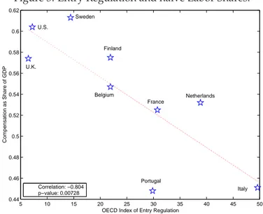
The empirical literature is silent on the impact of the economywide degree of com- petition on wages (or wage shares). To get an idea of whether the wage share might be increasing in competition (e.g. whether the wage share is decreasing in regulation), we regress a measure of entry regulation on the wage share for a group of OECD countries, as illustrated¹³ in Figure3. The correlation is highly negative (−0.804) and significant at the 1% level. Although this is only illustrative of the data, it is suggestive that wage shares in the data might indeed be increasing in competition. It is also consistent with the positive wage effect of competition suggested by Blanchard and Giavazzi (2003).

3.3.2 Comparative Statics II: Varying Parameters

Proposition3summarizes the impact of varying parameters on short-run equilibrium.

Proposition 3 In short-run equilibrium:

(i) labor market tightnessθis decreasing inb,ΦV,r,δ, andeχ;

(ii) unemployment is increasing inb,ΦV,r,δ, andeχ;

(iii) labor market tightness is decreasing inβ and unemployment is increasing inβ as long as σ>eσwhere

eσ≡

(1−τL)b+_q(θ)^ΦV _{(1−δ)(1−β)}¹ h_r+χ+βf(θ)

1−β +βf(θ)i

ΦV

q(θ) 1

(1−δ)(1−β)

h_r+χ+βf(θ)

(1−β) +f(θ)i .

2

The results of parts (i) and (ii) of Proposition3 are standard for search and matching models. Higher unemployment benefits, hiring costs, interest rates and separation rates all increase unemployment. Part (iii) merits comment. Unemployment increases in worker’s bargaining power (as is standard), unless the degree of competition is very low. The intu- ition is that when competition is low, higher worker’s bargaining power strengthens the

13The data on labor share is the compensation to GDP ratio taken from Gollin (2002), table 2, column 4. The data on entry regulation is the regulation index of Fonseca, et. al. (2001), table 2, column 4.

overhiring effect (i.e. increases firms’ incentives to hire more workers in the sense that

∂²wi

∂hi∂β− ^σ−1

(σ−β)² A h_i

Pi(yi)

P <0) so much, that the end result is lower unemployment.

3.4 Long-run General Equilibrium

Now we are ready to endogenize the degree of competition. In the long-run, firms may enter each industry by paying a real entry costΦEand by posting enough vacancies to hire the steady-state workforce. The details of firm entry and exit are as follows: Each period a measureδof firms exits, and is replaced by a measureδof new entrants¹⁴. New entrants begin production immediately with their steady-state workforce. Hence, we assume that entering firms know far enough in advance that they will be entering to complete all entry formalities. During this (these) pre-entry period(s) firms pay the entry cost. Because of the constant marginal vacancy posting cost they optimally post enough vacancies to hire their steady-state workforce immediately¹⁵. Entry by firms will continue until profits net of entry costs have been competed down to zero. Hence, free entry in the presence of barriers to entry leads to an equilibrium number of firmsn^∗, which is defined implicitly by:

ΦE(σ(n^∗)) +ΦV

h_i(σ(n^∗))

q(θ(σ(n^∗)))=VF(hi(σ(n^∗))). (28) The free entry condition states that the entry cost plus initial hiring costs must be amortized by profits over the firm’s expected lifespan. Since equilibrium profits are decreasing in competition ^∂V_∂σ^F <0, free entry forges a negative link between barriers to entry and the degree of competition/the number of firms in the economy¹⁶.

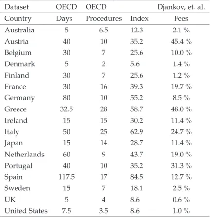
Entry barriers take two complementary forms, time and pecuniary costs. For 1997 we have detailed data on the number of business days it takes to set up a standardized OECD firm as reported by Pissarides (2003) and on entry fees as a percentage of per capita GDP from Djankov, et. al. (2002). We combine the two measures into a single one by adding up the entry costs as a percentage of monthly per capita GDP and the lost output of a single firm during the entry delay period. Formally, total barriers¹⁷to entry are found as:

ΦE(σ(n)) =d·y_i+ϕ·I(σ(n^∗)) (29)

14Recently, Felbermayr and Prat (2007) have extended our framework to allow for endogenous firm entry and exit. In their setup they distinguish between set-up costs and a fixed ’red tape’ cost that has to be paid every period that the firm is in operation. Thus they create endogenous firm exit. Based on estimation of their model for a panel of OECD countries they conclude that reducing regulatory cost for incumbent firms yields little employment gain.

15Note that it is not necessary to take the measureδof pre-entry firms into account in aggregate income. They do not yet produce, and only incur vacancy costs. Hence the firm’s profits and vacancy costs sum to zero.

16To forge an explicit link between barriers to entry and the number of firms, one may take two routes. We follow Blanchard and Giavazzi (2003) and assume thatσis an increasing function of the number of firms. Alter- natively, one may holdσconstant, and allow fornfirms competing via Cournot in each industry. In a previous version of this paper, we followed this second setup. Results are very similar to those of the simpler Blanchard and Giavazzi (2003) setup presented here, and are available upon request.

17 Our choice for the specification of entry barriers as proportion of output is driven by the data we have available. More precisely, we implicitly rule out the case in which there is a fixed fee to enter that does not depend on income. While such a fixed fee would pose no difficulty to include, we follow Blanchard and Givavazzi (2003) because the absence of fixed fees is analytically more convenient.

where d is the regulatory delay in months, y_i is firm-level output, ϕare entry fees as a percentage of monthly per capita GDP, andI(σ(n^∗))is aggregate income. Combining (29) with the free entry condition (28) yields:

d·yi+ϕ·I(σ(n^∗)) +ΦV

h_i(σ(n^∗))

q(θ(σ(n^∗)))=VF(hi(σ(n^∗))). (30) Equation (30) closes the long-run equilibrium. It determines the endogenous number of firmsn^∗and the degree of competitionσ(n^∗)in long-run equilibrium by defining a negative relationship between barriers to entry and the degree of competition in the long-run.

4 Quantitative Results

We are now in a position to calibrate our model and approach our quantitative questions.

We explore two alternative calibrations: a traditional calibration along the lines of Shimer (2005) and a small surplus calibration similar to that in Hagedorn and Manovskii (2008).

For each calibration we ask: What is the impact of increasing competition on equilibrium unemployment and wages? In order to answer the question, we run policy experiments designed to assess whether the product market deregulation of the late 1970’s and early 1980’s could account for the subsequent decline in US unemployment during the 1980’s and 1990’s. In addition, we examine whether other factors, such as the decline in labor taxation or the waning of union bargaining power could account for the decline in unemployment.

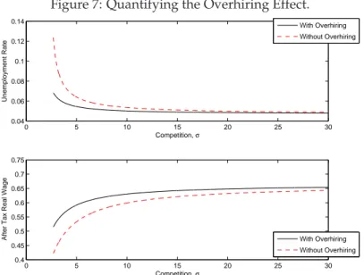
Finally, we go on to quantify the overhiring effect.

4.1 Calibration

Our model period is one month. All parameters for both the traditional and the small surplus calibration are reported in Table4. In both cases, we calibrate the model to US data in 1998.

The majority of parameters is common to both calibrations. We normalize the level of technologyAto unity. Our choice of 4.0% for the annualized real interest rate is standard.

We set the job-finding rate f(θ) to be 0.45 monthly following Shimer (2005), and target the 1998 HP-trend value for unemployment of 5.1%¹⁸by setting the total separation rate χ=0.024monthly, roughly in line with the estimates in Shimer (2005). We setδ=0.8%, so that the monthly probability that a firm will cease to exist implies an annual firm survival rate of 90.8%. This matches the average five-year survival probability reported by Wagner (1994) and is in line with the four-year survival probabilities reported in Mata and Portugal (1994), which imply monthly exit rates between 0.6 and 1.4%. We set worker’s bargaining power so thatβ=0.50¹⁹, in line with the estimates of Abowd and Allain (1996) and Yashiv

18We wish to concentrate on the long-run impact of regulation, abstracting from business cycle considerations.

Hence, we use the HP-trend value, in which the business cycle component has been filtered out using a smoothing parameter of1e6.

19Hagedorn and Manovskii (2008) chooseβto match the wage elasticity of productivity. They obtain a very small value ofβ=0.052. We will discuss the impact of such low values of bargaining power on our results later in the paper.

(2001). We let the matching elasticity take the value, η=0.50²⁰, in the range reported by Petrongolo and Pissarides (2001). We also chooseq(θ) =0.238, as in den Haan, Ramey and Watson (2000). Our choices for job-finding and job-filling rates pin down US equilibrium labor market tightness in 1998 to beθ= _q(θ)^f(θ)=1.89.²¹ This value for tightness looks high at first glance. However, it is necessary to adjust for the fact that firms open as many va- cancies as necessary in order to fulfill their hiring needs in expectation. If we multiply the equilibrium tightnessθwith the firm’s matching rate, we find a ratio of open jobs to unem- ployed of 45%, in line with the findings of Shimer (2005). We set the scaling parameter of the matching function to satisfys=_θ^f_1−η^(θ). In both the traditional and small surplus baseline calibrations, we set labor taxes to 32% to match the 1998 labor wedge reported in Prescott (2002)²². Tax revenues are redistributed to households in the form of lump-sum transfers.

Finally, we need to parameterize the function relating demand elasticity to the number of firms. In a fully microfounded formulation of Cournot competition within industries²³, the demand elasticity faced by the firm is given byσ·n, wherenis the number of firms. For this reason, we chooseg(n) =nand normalizeσ=1.

4.1.1 Traditional vs Small Surplus Calibration

At this point, we are left with a short-run equilibrium condition (24) which relates the util- ity from unemployment b to the vacancy posting costs ΦV. We first decompose ²⁴ total utility from unemploymentb into an unemployment benefits componentb_band a home production or leisure componentbh, so thatb=bb+bhNext, we choose the benefits compo- nentb_b=0.187so that the net benefit replacement rate_w(1−τ^bb

L)=0.30, in line with US data.

Finally, for the traditional calibration we choose the home production or leisure component b_h=0.198so that the model’s semi-elasticity of unemployment with respect to benefits is equal to 2.0, as estimated by Costain and Reiter (2008). The resulting total replacement rate

w(1−τb L) is 0.62.

In the small surplus calibration, targeting a semi-elasticity of benefits of 14.0 leads to a home production component of benefits of b_h=0.326and a total replacement rate

w(1−τb L) =0.95, as in Hagedorn and Manovskii (2008). Hence, the only difference between the traditional and small surplus calibrations is the home production component of utility b_hand hence the total utility from unemploymentb.

20In a previous version of the paper, we established that the Hosios (1990) condition is a necessary but not a sufficient condition for efficiency in our setup. As the demand elasticity goes to infinity, the economy converges to the perfect competition limit in which the Hosios condition holds.

21Pinning down the value ofθdoes not fully describe short-run equilibrium, as long as some other variables or parameters are left free. In our case, these parameters will beΦVandb.

22We also looked at a setting with both a labor tax and a consumption tax, and the results were very similar.

23cf. Galí and Zilibotti (1994) for such a framework.

24Due to linear utility, of course, only the total utility from unemploymentbmatters for our calibration. The breakdown into benefit and home production components will be useful later, however, in the policy experiments.

4.1.2 Entry Costs

For 1997, we can use the detailed entry cost data reported in Table 1, resulting in entry costs for the US corresponding to 0.6 months of aggregate per capita income. Djankov, et. al. (2003) report entry fees of 1.0% of annual per capita income, or 12% of monthly per capital income. Pissarides (2003) compiles an index for entry delay as the number of business days it takes (on average) to fulfill entry requirements, weighted by the number of procedures that must be performed. The US entry delay index is 8.6 days, or 0.47 months of lost output, based on 220 business days in a year. Adding the two measures yields total entry costs equal to 0.59 months of output. In what follows, we will call our composite measure of entry fees and entry delay costs for 1997 the Djankov/Pissarides index.

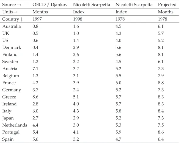
For 1978, such detailed entry cost data is unavailable. However, Nicoletti and Scarpetta (2003) have compiled an index on product market regulation for a set of 21 countries whose starting date is 1978 and whose ending date is 1998. These 1978 and 1998 index values are displayed in the middle columns of Table 2for the subset of 17 countries for which both Nicoletti and Scarpetta (2001)’s panel index for 1978-1998 and the detailed cross section data for 1997 is available.

In order to estimate US entry costs, we use a triangulation procedure. To estimate entry costs in 1978, we first run the following regression:

Djankov/Pissarides_1997,i=α0+α1·Nicoletti/Scarpetta_1998,i+εi. (31) The results of the regression are reported in Table3. We first note that the correlation be- tween Nicoletti and Scarpetta’s index in 1998 and our combined Pissarides/Djankov index (first column of Table2) is very high at 0.77. Hence, both indices seem to be measuring the same things. The estimate ofαb1is highly significant, with at−Statistic of 4.7, while the estimate forαb0is marginally significant. Next, we use the estimatesαb0andαb1to transform the Nicoletti and Scarpetta index value for 1978 into a Djankov/Pissarides-style index for 1978, by taking

Djankov/Pissarides_1978,i=αb0+αb1·Nicoletti/Scarpetta_1978,i. (32) The results of the projection (32) are displayed in the last column of Table2. For the US, the resulting measure of entry costs for 1978 is 5.2 months of per capita output, a nearly 9-fold increase relative to 1997.

4.1.3 Baseline 1998 Calibrations

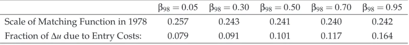
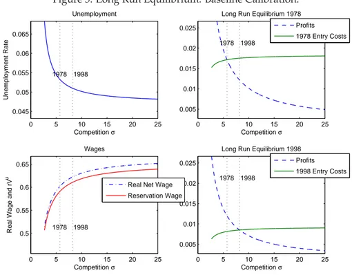
The results of the traditional and small surplus baseline calibrations to the US economy in 1998 are presented in Figures5 and6 respectively. The bottom right panel of Figure5 shows that under the traditional calibration, 1998 US entry cost and profits are equalized when demand elasticityσis 8.2, which corresponds to a markup of 7.0%²⁵. The bottom right panel of Figure6shows that under the small surplus calibration, the 1998 US long- run equilibrium implies a demand elasticity of 18.8 and a somewhat smaller markup of

25Under individual bargaining, the markup is given by^σ−β_σ−1.

2.8%²⁶. The 7% markup lies well within the typical 5%–15% range of reported markups, e.g. Martins et al, (1996) or Rotemberg and Woodford, (1995).

Figures5and6also show how unemployment and wages respond to varying degrees of product market competition. As expected, unemployment is decreasing and real wages are increasing in competition, where competition is measured as demand elasticityσ. We note that the bulk of the impact of monopoly power on wages and unemployment occurs under very low levels of demand elasticity. This is consistent with the empirical results of Bresnahan and Reiss (1991), who find that most of the benefits to increased competition come from the entry of the first three to five competitors, with very little benefits accruing to further entry.

4.2 Product Market Deregulation and the Labor Market

We now use the model to run a policy experiment, in order to assess to what extent product market deregulation can directly account for the decline in U.S. unemployment during the 80’s and 90’s. We do this by taking the 1998 US baseline model calibrated above as a starting point, and then examining the impact of raising entry costs to 1978 levels. We emphasize that we are interested in matching the unemployment differential from HP-trend data from which the business cycle component has been filtered out, in line with our focus on the long-run impact of a change in product market regulation.

To run the experiments, we hold the utility from home productionb_hfixed in 1998 and 1978, and adjustb_bso that the benefit replacement rate _w(1−τ^bb

L) remains fixed at 30%. All other parameters are held fixed at their 1998 levels.

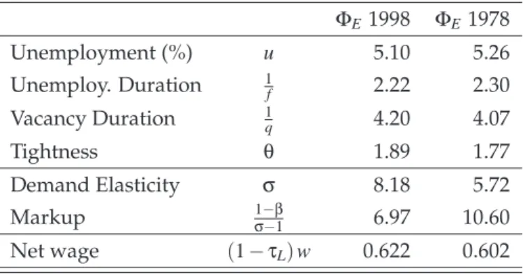
Results of the deregulation policy experiment are presented in Tables5 and6. In the traditional calibration, changes in product market regulation can only account for a sur- prisingly small change in equilibrium unemployment. Raising entry costs nearly nine-fold to their 1978 levels does lead to a substantial decrease in competition, causing markups to increase by about 50%, from 7.0% to 10.6%. The resulting increase in unemployment is very small, however, at less than two-tenths of one percentage point, causing unemployment to rise from 5.10% to 5.26%. In contrast, in the data, trend unemployment increases from 5.1%

in 1998 to 7.2% in 1978, as shown in Figure1.

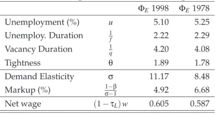
Under the small surplus calibration, however, we find that product market deregula- tion can account for nearly the entire decrease in unemployment between 1978 and 1998. In particular, raising entry costs to their 1978 levels causes unemployment to rise from 5.10%

to 7.2%, an increase of 2.1 percentage points²⁷. However, the small surplus calibration is controversial, as it is inconsistent with evidence on the semi-elasticity of unemployment with respect to benefits (Costain and Reiter, 2008) and furthermore implies implausibly large labor supply elasticities at the extensive margin (Haefke and Reiter, 2006). This ten- sion between the small and large surplus calibration is the same as in the unemployment

26The greater degree of equilibrium competition (higherσ) and lower markups are due to the smaller profits in the small surplus calibration.

27Markups increase from 2.8% in 1998 to 6.9% in 1978.