Expanding the Scope of Impedance Spectroscopy for the Analysis of Adherent Cells: Electrode Material, Electrode Design, and Data Analysis

Expanding the Scope of Impedance Spectroscopy for the Analysis of Adherent Cells: Electrode Material, Electrode Design,

and Data Analysis

DISSERTATION

zur Erlangung des Doktorgrades der Naturwissenschaften (Dr. rer. nat.) der Fakultät für Chemie und Pharmazie

der Universität Regensburg

vorgelegt von Christian Götz aus Regensburg

2017

Die vorliegende Arbeit wurde in der Zeit von Januar 2013 bis Oktober 2017 unter der Gesamtleitung von Prof. Dr. Joachim Wegener am Lehrstuhl für Analytische Chemie, Chemo- und Biosensorik der Universität Regensburg angefertigt.

Prüfungsgesuch eingereicht am: 13. Oktober 2017 Tag der mündlichen Prüfung: 05. Dezember 2017

Prüfungsausschuss: Vorsitzender: Prof. Dr. Hubert Motschmann

Erstgutachter: Prof. Dr. Joachim Wegener

Zweitgutachter: PD Dr. Rainer Müller

Drittprüfer: Prof. Dr. Antje Bäumner

This work was financed and supported by Fraunhofer EMFT.

“For a successful technology reality must take precedents over public relations for nature cannot be fooled.”

— Richard Feynman

to Thea and my family

Outline i

O ^UTLINE

I Introduction ... 1

1 Adherent Cells as Physiological In Vitro Model ... 1

2 Conducting Polymers − Beginnings and Recent Advances in Biosensing... 8

3 Objective ... 15

II Theory ... 17

1 Impedance Spectroscopy in Aqueous Media ... 17

2 Conducting Polymers as Electrode Material ... 34

3 Regression Analysis ... 41

III Experimental and Theoretical Studies ... 49

1 Materials and Methods ... 49

2 PEDOT:PSS as Electrode Material for Impedance-based Cellular Assays ... 72

3 Bipolar Electrodes ... 138

4 Derivative Impedance Spectroscopy (DIS) ... 168

5 Summary ... 195

IV References ... 201

V Appendix ... 211

1 List of Abbreviations ... 211

2 Supplementary Information ... 213

3 LabView Programs ... 217

4 Publications and Presentations ... 224

5 Acknowledgements ... 225

Table of Contents i

T ^{ABLE OF} C ^ONTENTS

I Introduction ... 1

1 Adherent Cells as Physiological In Vitro Model ... 1

1.1 Label-Free Whole-Cell Biosensors ... 1

1.2 Immobilizing Cell Monolayers on Transducer Surfaces ... 4

2 Conducting Polymers − Beginnings and Recent Advances in Biosensing... 8

2.1 Short History of Conducting Polymers ... 8

2.2 Conducting Polymers in Biosensing ... 11

3 Objective ... 15

II Theory ... 17

1 Impedance Spectroscopy in Aqueous Media ... 17

1.1 Electrical Current: Theory ... 17

1.2 Electrical Current: Practical Considerations ... 21

1.3 The Electrode-Electrolyte Interface ... 23

1.4 Electric Cell-Substrate Impedance Sensing (ECIS) ... 27

2 Conducting Polymers as Electrode Material ... 34

2.1 Intrachain Charge Transport ... 34

2.2 Interchain Electron Hopping ... 37

2.3 The Electrode-Electrolyte Interface of PEDOT:PSS ... 39

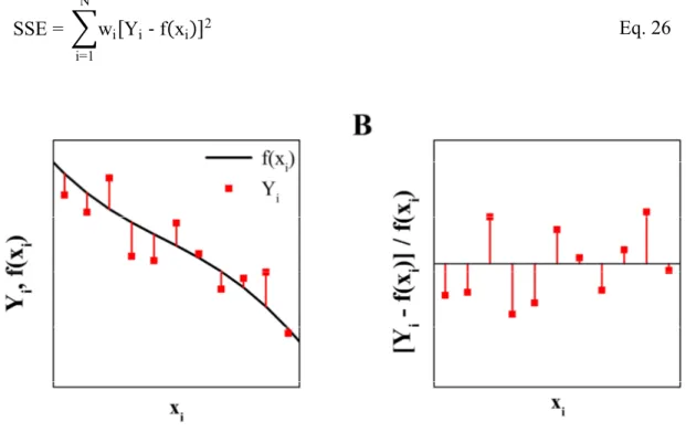
3 Regression Analysis ... 41

3.1 General Approach ... 41

3.2 Determination of the Boundary Conditions ... 43

3.3 Fitting Method: The Hyperfunnel Algorithm ... 45

III Experimental and Theoretical Studies ... 49

1 Materials and Methods ... 49

1.1 Cell Culture Techniques ... 49

1.1.1 Cell Culture Conditions ... 49

1.1.2 Cell Lines ... 50

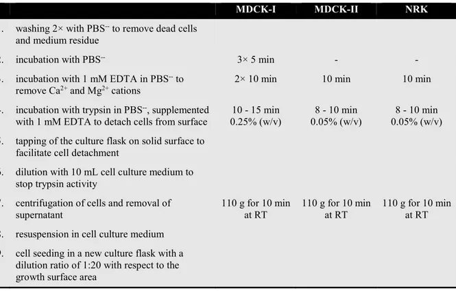
1.1.3 Subcultivation ... 51

1.1.4 Cryopreservation and Recultivation ... 52

1.1.5 Live/Dead Staining ... 52

1.2 Impedance Spectroscopy... 53

1.2.1 Experimental Setup ... 53

1.2.2 Basic Experimental Procedure ... 54

1.2.3 Electrode Layouts ... 54

1.2.4 Equivalent Circuits ... 55

1.2.5 Data Presentation ... 57

Impedance Spectra and Time Course ... 57

Errors ... 58

1.3 Electrical Cell Manipulation ... 59

1.3.1 Electroporation ... 60

1.3.2 Wounding ... 60

1.4 Micromotion ... 61

1.4.1 Power Spectral Density (PSD) Analysis ... 61

1.4.2 Detrended Fluctuation Analysis ... 64

1.4.3 Detrended Variance Analysis (DVA) ... 67

1.5 LabVIEW Programs ... 67

1.5.1 Simulation ... 68

1.5.2 Manual Fitting ... 69

1.5.3 Regression Analysis ... 69

1.5.4 Regression Analysis Evaluation ... 70

Table of Contents iii

2 PEDOT:PSS as Electrode Material for Impedance-based Cellular Assays ... 72

2.1 Objective ... 72

2.2 Materials and Methods ... 72

2.2.1 Screen Printing ... 72

2.2.2 Electrode Design ... 73

2.2.3 Electrode Preparation for Impedance-based Assays ... 75

PEDOT:PSS Electrodes ... 75

Gold Electrodes ... 76

2.2.4 Electrode Characterization ... 76

Determination of the Physical Dimensions ... 76

Optical Characterization ... 77

Impedimetric Characterization and Parameter Fitting ... 77

Determination of the Parasitic Impedance ... 78

Influence of the Cell Culture Medium on the Electrode Impedance ... 79

Long-Term Stability Upon Storage in Ambient Air ... 80

Voltage Dependence ... 80

2.2.5 Cell Adhesion, Cytochalasin D, and Saponin Treatment ... 80

2.2.6 Proliferation ... 81

2.2.7 Cytotoxicity Assay for Saponin ... 82

2.2.8 Micromotion ... 83

2.2.9 Electroporation ... 83

2.2.10 Comparison of MDCK-I, MDCK-II, and NRK Cells ... 84

2.3 Results and Discussion ... 84

2.3.1 Electrode Characterization ... 84

Determination of the Physical Dimensions ... 84

Optical Characterization ... 86

Impedimetric Characterization ... 88

Determination of the Parasitic Impedance ... 90

Influence of Cell Culture Medium on the Electrode Impedance ... 92

Long-Term Stability Upon Storage in Ambient Air ... 95

Voltage Dependence ... 96

2.3.2 Comparison of Impedance Spectra of MDCK-II cells recorded with PDT and 8W10E Electrodes ... 98

2.3.3 Cell Adhesion and Spreading ... 104

Time Course of Impedance Magnitude, Resistance and Capacitance ... 104

Analysis of the Cell Parameters C

, α, and R

during the Adhesion and Spreading of MDCK-II Cells ... 106

Optical Study of Adhesion and Spreading ... 109

Conclusion ... 111

2.3.4 Cytochalasin D Treatment ... 111

2.3.5 Proliferation ... 113

2.3.6 Cytotoxicity Assay: Saponin ... 115

2.3.7 Micromotion ... 117

2.3.8 Electroporation ... 125

2.3.9 Comparison of MDCK-I, MDCK-II, and NRK Cells ... 130

2.4 Summary and Outlook ... 135

3 Bipolar Electrodes ... 138

3.1 Introduction ... 138

3.2 Objective ... 139

3.3 Materials and Methods ... 140

3.3.1 Photolithography ... 140

3.3.2 Electrode Design ... 141

Bipolar Electrodes Category 1 ... 141

Bipolar Electrodes Category 2 ... 143

3.3.3 Electrode Preparation and Cell Manipulation ... 144

3.3.4 Wounding ... 145

Table of Contents v

3.4 Results and Discussion ... 145

3.4.1 Bipolar Electrodes Category 1 ... 145

Characterization of Open Bipolar Electrodes ... 145

Comparison of Electrodes with Different Potentials ... 146

Wounding ... 147

Discussion ... 150

3.4.2 Bipolar Electrodes Category 2 ... 152

Analysis of Impedance Spectra ... 152

Cell Attachment and Spreading ... 155

Determination of the Electrode and Cell Parameters ... 156

Simulation of Impedance Spectra with Discrete Bipolar Electrode Resistances ... 159

Simulation of Impedance Spectra of Different Cell Types on Bipolar Electrodes ... 162

Discussion ... 165

3.5 Summary and Outlook ... 166

4 Derivative Impedance Spectroscopy (DIS) ... 168

4.1 Introduction ... 168

4.2 Objective ... 170

4.3 Materials and Methods ... 172

4.3.1 Regression Analysis of Derivatives ... 172

Simulation and Differentiation of Impedance Spectra ... 172

Noise Simulation ... 173

Evaluation of the Fit Results ... 175

4.3.2 Discrimination of α and R

in the Impedance Spectrum ... 178

Looking for a Sensitive Frequency ... 179

Zero Migration ... 182

4.4 Results and Discussion ... 182

4.4.1 Simulation of Derivative Spectra ... 182

4.4.2 Regression Analysis of Derivatives ... 184

4.4.3 Discrimination of α and R

in the Impedance Spectrum ... 190

Looking for a Sensitive Frequency ... 190

Zero Migration ... 192

4.5 Summary and Outlook ... 193

5 Summary ... 195

5.1 English Summary ... 195

5.2 Deutsche Zusammenfassung ... 197

IV References ... 201

V Appendix ... 211

1 List of Abbreviations ... 211

2 Supplementary Information ... 213

3 LabView Programs ... 217

3.1 Simulation and Manual Fitting of Impedance Spectra... 217

3.2 Simulation of Time Series with Different Noise Colors ... 218

3.3 Micromotion Analysis ... 219

3.4 Simulation of Derivative Impedance Spectra ... 220

3.5 Fitting of Impedance Spectra ... 221

3.5.1 Fitting of Single Spectra Using the Hyperfunnel Algorithm ... 221

3.5.2 Batch Fitting using the Hyperfunnel Algorithm ... 222

3.5.3 Analysis of the Results Generated by Batch Fitting ... 223

4 Publications and Presentations ... 224

4.1 Patents ... 224

4.2 Conferences ... 224

5 Acknowledgements ... 225

1 1 Adherent Cells as Physiological In Vitro Model

I I NTRODUCTION

1.1 Label-Free Whole-Cell Biosensors

The development of a new drug from its first synthesis until the introduction into the market is difficult, costly, and time-consuming. Out of every 5000 to 10000 newly synthesized potential drugs only 9 reach the clinical trial phase, and 1 enters the market. Including all developmental and clinical phases, this leads to an estimated cost for one new drug that gets successfully launched of about 1.8 billion US-Dollars. This high cost has led to a decline of the number and quality of innovative, cost-effective new drugs over the last years. One of the major challenges and opportunities for pharmaceutical research and development is the identification of bad candidates in the early phase of drug discovery. Lack of efficacy and ‘off-target’ toxicity that surface not until one of the highly expensive clinical stages are among the main reasons for late phase attrition, i.e. dropout of a potential compound. Shifting the identification of compounds with inappropriate drug-like properties to an earlier phase would significantly reduce the cost and improve the efficiency and productivity of the drug development process.

Analytical tools that are both label-free and based on whole-cell biosensor techniques exhibit

several advantages compared to classical methods to tackle that problem. Conventional ligand

affinity assays mainly address the binding affinity between a ligand and a receptor or the

inhibition of an enzyme.

The respective biomolecules are usually immobilized on the surface

of multi-well plates or microbeads. Readout methods include radiometric as well as

colorimetric and fluorimetric techniques. Whole-cell biosensors on the other hand use cells as

recognition element and thus reveal functional information about the impact of a stimulus on a

living system. They are not limited to a single event like receptor-ligand interaction, but mirror

the complexity of the signal pathway of a whole cell. As a consequence, the measurements may elucidate signal transduction pathways and drug mechanisms, and provide information on the effectiveness, selectivity, and cytotoxicity of an analyte. In addition, it opens the possibility to discover new off-target signaling pathways involved in a drug response during the screening.

6

In the recent years, label-free technologies have gained increasing importance in the field of cell-based drug discovery and high throughput screening. Reduced cost, improved throughput, increased sensitivity, and more sophisticated data analysis have led to more acceptance in research and industry.

Traditionally, tags, dyes, or genetically engineered cell lines are employed in label-based whole-cell assays. However, they have been criticized to compromise the outcome of the measurements due to cross-reactions and altered cell behavior. The labeled approaches are mostly end-point assays that contain no information on the kinetics, so that critical data may be missed. Moreover, waste disposal and health hazard issues have to be considered, especially when using radioactive probes or potentially cancerogenic DNA-binding labels. By contrast, label-free assays – as per definition – do not require tags or labeling, and in addition support time-resolved measurements. Generally speaking, label-free whole-cell assays provide a biologically more relevant environment and are a good trade-off between research on whole organisms, which raises ethical as well as financial challenges, and biochemical in vitro assays.

On the other hand, whole-cell sensors are often considered to be a “black box” as only an overall response of the cell is transmitted.

Detailed mechanistic studies about the molecular processes inside the cell can – if at all – only be performed with considerable effort and exhaustive controls. This is why research in that field is often complemented with classical microscopy and fluorescence labeling. Despite substantial improvements over the last years, cost of instruments and plates, as well as low throughput are still the most substantial obstacles to comprehensive use of label-free technology in drug screening, as conveyed in a survey from 2010.

Consequently, these technologies are rarely used for high throughput screening, but rather during the subsequent hit to lead optimization. The hit to lead phase is an early stage during drug discovery where hits from the primary screening phase are verified, evaluated, and further optimized.

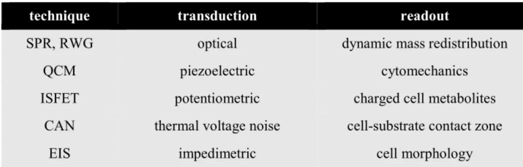
Some of the most relevant label-free techniques are summarized in Tab. I-1.

Different sensor

techniques address different features of a cell and must be chosen accordingly. SPR (surface

plasmon resonance) and RWG (resonant waveguide grating) use the dependence of surface

plasmons (electron oscillations) on a metal surface on the refractive index in the adjacent

medium as sensor principle. The evanescent field generated by the surface plasmons has a

3 1 Adherent Cells as Physiological In Vitro Model

penetration depth of about 200 nm. It is, therefore, able to detect changes of the refractive index at the bottom of adherent cells, caused for example by a rearrangement of the cytoskeleton or other cellular components. The term dynamic mass redistribution has been established for these rearrangements inside the cell.

The detection method of a QCM (quartz crystal microbalance) is based on the principle that the resonance frequency and the amplitude of shear wave oscillations of a piezoelectric quartz crystal depend on the mass and viscoelasticity of the material deposited on the quartz. Changes in the cytomechanical properties of the cell can thus be monitored with high sensitivity.

Some semiconductor based biosensors have been developed that employ the same principles as a MOSFET (metal oxide field-effect transistor).

In an ISFET (ion-selective field-effect transistor) the gate consists of an ion-selective membrane that is electrically connected to a reference electrode via the electrolyte. At constant gate and drain voltage, the concentration of the ions specified by the selective layer modulates the drain current. The main application of this method is the monitoring of changes in the extracellular pH value.

Transistors have also been used to examine the voltage peaks caused by neuronal action potentials.

Non-electrogenic cells could be studied by analysis of the thermal noise caused by cells growing on top of a MOSFET.

This eventually led to the development of the relatively new CAN (cell adhesion noise) spectroscopy, that is yet to be commercially established. By quantitative interpretation of the thermal noise in the cell- substrate junctions, a silicon chip consisting of an array of several thousand transistors with sub-cellular dimensions is used to produce time-resolved images of cells adhered on its surface.

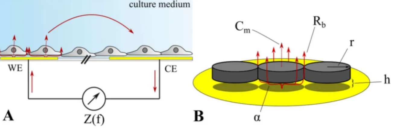
In EIS (electrochemical impedance spectroscopy) an alternating voltage is applied between two

coplanar film-electrodes immersed in an electrolyte. The alterations in the impedance caused

by cells growing on top of the electrodes is analyzed in a frequency dependent manner. EIS is

the most versatile of these methods as numerous electrode layouts exist to address different

aspects of cell analysis. Especially the widely-used ECIS™ (electric cell-substrate impedance

sensing) method allows for a detailed analysis of the cell-cell junctions, the cell-substrate

contacts, and the cell membrane. This is due to its defined electrode layout with a small working

electrode and a larger counter electrode, as well as the in-depth mathematical model developed

by Giaever and Keese (cf. II.1.4 for more details).

Based on this pioneering work, several

other technologies have emerged. The xCelligence system by ACEA Biosciences uses arrays

with interdigitated electrodes that are designed to cover a uniquely large portion of the well

area. Thus, the impedance signal is averaged over a greater number of cells and may

consequently show less well-to-well variations.

Their system is promoted with an emphasis

on the analysis of beating cardiac cells because of its particularly fast data acquisition rate (Real Time Cell Electric Sensing, RT-CES).

Molecular Devices has released a 384-well cell analysis system with strong focus on high throughput. The corresponding measurement technique is termed CDS (cellular dielectric spectroscopy).

Tab. I-1: Label-free biosensing techniques used to monitor cell-based assays (SPR = surface plasmon resonance, RWG = resonant waveguide grating, QCM = quartz crystal microbalance, ISFET = ion- selective field-effect transistor, CAN = cell adhesion noise spectroscopy, EIS = electrical impedance spectroscopy).

technique transduction readout

SPR, RWG optical dynamic mass redistribution

QCM piezoelectric cytomechanics

ISFET potentiometric charged cell metabolites

CAN thermal voltage noise cell-substrate contact zone

EIS impedimetric cell morphology

1.2 Immobilizing Cell Monolayers on Transducer Surfaces

Aside from the measurement technique the choice of the cell line needs to be considered for compound testing. Immortalized cell lines are cell populations that proliferate indefinitely due to natural or artificial mutation. They are cheap, easy to grow, and reproducible. Primary cells, taken directly from living tissue, represent the respective biological systems more accurately, but require significantly more effort to grow and keep in culture.

For this reason, immortalized cells are often preferred over primary cells. Depending on the target of the drug or the analyte under test there are cell lines derived from the targeted tissue that are used as model systems.

Tab. I-2 shows exemplarily some immortalized epithelial cell.

5 1 Adherent Cells as Physiological In Vitro Model

Tab. I-2: Selected immortalized cell lines and typical applications as model system (HUVEC = Human Umbilical Vein Endothelial Cells, Caco = adenocarcinoma of the colon, MDCK = Madin-Darby Canine Kidney, NRK = Normal Rat Kidney).

cell line origin model system for source

HUVEC human vein endothelium^a vascular inflammation ²³

Caco-2 human colon epithelium intestinal drug absorption ²⁴

MDCK canine kidney epithelium epithelial water and solute transport ²⁵

NRK rat kidney epithelium nephrotoxicity ²⁶

Epithelia are a type of interfacial tissue that lines all inner and outer surfaces of the body.

Epithelial tissues serve as protective barrier (skin), take up nutrients (intestine), control the transport of ions, metabolites, and proteins (blood vessel, intestine, kidney), or perform sensory tasks

(retinal pigment epithelium, auditory hair cells, olfactory epithelium). Growing in two- dimensional cell monolayers, they are particularly well suited for in vitro analyses. It is generally assumed that the interactions of cells with the surrounding tissue in vivo and technical in vitro surfaces rely on the same principles. When a cell suspension is placed inside a well, the cells sediment and get close to the surface, where they establish molecular contact with proteins immobilized on the surface. These proteins can be either artificially deposited on the surface or be excreted by the cells themselves. Especially positively charged polymers like poly-L-lysine facilitate surface adhesion due to electrostatic attraction between the polymer and the overall negatively charged membrane surface of cells. Proteins contained in physiological cell growth buffers or media also adsorb quickly on hydrophilic surfaces and support cell adhesion. Once the initially spherically shaped cells have adhered (or attached) to the substrate, they start to spread out and increase the contact area, followed by the formation of cell-cell contacts with their neighboring cells.

In a fully established cell monolayer several proteins and other biopolymers are involved in keeping its functional and structural properties intact (Fig. I-1). Between the cells and the substrate is the subcellular cleft with the extracellular matrix (ECM). The average distance between cell and substrate is between 25 nm and 200 nm, depending on the cell type and the substrate coating. The ECM is a highly heterogeneous macromolecular network of proteins, carbohydrates, proteoglycans, glycoproteins, and other biomolecules. The cells are anchored to the ECM via surface receptor proteins that recognize certain amino acid sequences in ECM proteins. The most common surface receptor proteins are the integrins. They are transmembrane

a Endothelial cells are a subtype of epithelial cells lining the blood vessels.

proteins that are linked to the cytoskeleton via adapter proteins on the intracellular side and, for example, to the ECM protein fibronectin with its well-known RGDS amino acid sequence on the extracellular side of the membrane. This provides adhesive strength and prevents the anchorage proteins from being torn out of the cell membrane when the cell is exposed to mechanical stress.

Fig. I-1: Schematic of epithelial cells growing as confluent two-dimensional monolayer (not drawn to scale). The cytoskeletons of individual cells are joined via adherens junctions and desmosoms, and linked to the ECM (extracelluar matrix) via transmembrane proteins called integrins. This provides mechanical stability and adhesion strength. The cytoskeleton – consisting of intermediate filaments (blue), actin filaments (red), and microtubuli (not shown) – defines the overall shape of the cells and supports also the microvilli (only shown in the right cell). The tight junctions ensure the polarity of the cell (fence function) and prevent molecules from crossing the cell layer on the paracellular pathway (gate function).²⁹

In a similar fashion, the cytoskeletons of adjacent cells are interconnected via transmembrane proteins of the cadherin family. One usually distinguishes between the adherens junctions, that link the actin filaments, and the desmosomes, that connect the intermediate filaments of neighboring cells. Both have very distinct functions related to cell shape and tensile strength.

The cytoskeleton continuously extends across the whole epithelium, thus providing a particularly high mechanical stability.

The uptake or release of nutrients, ions, or metabolites through an epithelium is firmly regulated

by the cells via transport proteins. The establishment of chemical and electrochemical gradients

across the cell layer allows the active control of the transport processes required for the

functionality of the cell layer. One example is the transport of glucose from the gut into the

intestinal epithelium, driven by a Na

-gradient, before it is further passed on to the underlying

tissue. It is therefore highly important to prevent free diffusion across the cell layer on the

paracellular pathway, i.e. through the intercellular cleft. This is accomplished by the tight

7 1 Adherent Cells as Physiological In Vitro Model

junctions, barrier proteins that are located close to the apical pole of the cell which seal the

intercellular cleft (gate function, Fig. I-1). The second purpose of the tight junctions is that

proteins integrated in the membrane cannot diffuse from the basal membrane side to the apical

membrane side or vice versa (fence function). Thereby, the functional polarity of the cell is

preserved.

2.1 Short History of Conducting Polymers

Polymers are not simply electrically non-conducting insulators, but cover the whole spectrum between insulating materials and plastics with metal-like behavior. In 2000 Shirakawa, Heeger, and MacDiarmid received the Nobel prize for the “discovery and development of electrically conductive polymers”.

Based on Kekulé’s discovery of the electron structure of benzene around 1860 with its delocalized π-system, the idea had come up that electrons could be delocalized not only in cyclic molecules but also in polyconjugated organic chains, which should lead to electrical conductivity. The simplest polymer exhibiting such a structure is polyacetylene (Fig. I-2).

Fig. I-2: Chemical structures of trans- and cis-polyacetylene

Polyacetylene was first synthesized by Natta in 1958 as black, air-sensitive, insoluble, and

infusible powder which did not attract much attention.

Even after Shirakawa was capable of

controlling film formation and cis/trans-configuration of the polymer in the 1970s, its

conductivity was still in the range of an insulator in case of cis-polyacetylene and in the range

of a poor semiconductor in case of trans-polyacetylene.

It was not until 1977 when Heeger

and MacDiarmid discovered that by modifying polyacetylene with halogens its conductivity

could be increased by several orders of magnitude.

This process, called doping, leads to partial

oxidation of the double bonds and is essential for the conductivity of the polymer. By

mechanically stretching polyacetylene films its conductivity could even be increased to match

that of silver or copper.

However, as doped PA loses its conductivity upon exposure to oxygen

in ambient air, it has barely any significance nowadays.

Instead, other polymers like

polypyrrole, polyaniline, or polythiophene and its derivative, poly(3,4-ethylenedioxythio-

9 2 Conducting Polymers − Beginnings and Recent Advances in Biosensing

phene) (PEDOT), have attracted much interest and are widely used in research and industrial applications (Fig. I-3).

Fig. I-3: Chemical structures of the most relevant conducting polymers: polyaniline, polypyrrole, polythiophene, and PEDOT. PEDOT exhibits high electrochemical stability due to the blocked 3- and 4- positions of the thiophene ring by a dioxyethylene bridging group.

PEDOT for example has been used as antistatic

and sensor material

, as hole injection layer in electroluminescent devices

, and in photovoltaic cells

. Organic conducting polymers combine the electrical properties of metals and semiconductors with the mechanical properties and processability of polymers. Moreover, they can be derivatized to modify their mechanical, chemical, electrical, or optical properties.

Derivatization can either be accomplished via synthetic chemistry at the monomer itself or by choice and concentration of the dopant. The best example is PEDOT. Conductive polymers are usually quite insoluble in any solvent and thus difficult to handle. By doping with the negatively charged copolymer poly(styrene sulfonate) (PSS) PEDOT gets dispersed in the aqueous reaction solution during polymerization.

PEDOT:PSS is commercially available as an aqueous dispersion which can easily be coated

onto any substrate. The researchers initially developed PEDOT to be a water soluble polymer

with blocked β-positions to prevent undesired cross-couplings. However, PEDOT itself was

found to be an insoluble polymer and exhibited a high conductivity (300 S/cm), stability, and visible light transmittance in thin films. Dispersability was finally achieved with the afore mentioned PEDOT:PSS, exhibiting good conductivity (10 S/cm), next to excellent degradation stability and transparency for visible light.

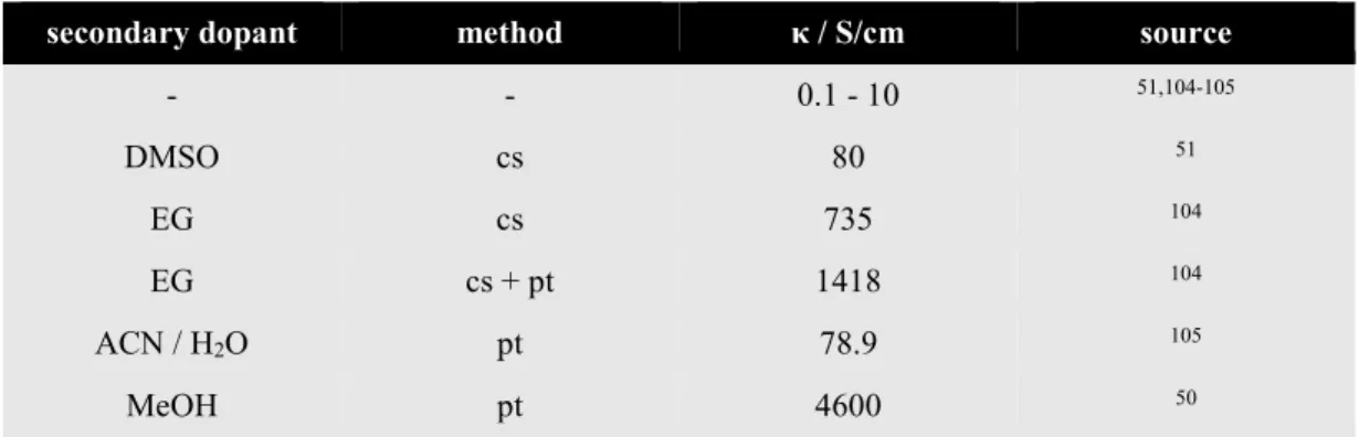
In the recent years the conductivity of PEDOT:PSS has been enormously increased by certain additives or processing techniques that lead to morphological changes within the polymer structure (Tab. I-3, cf. II.2.2 for more details). PEDOT:PSS shows properties of a supercapacitor as it forms a swollen hydrogel in aqueous solutions, hence generating a huge effective surface area.

This makes it particularly interesting for applications where the electrode-electrolyte interface plays an important role, like for example in biosensors.

Fig. I-4: Chemical structure of PEDOT:PSS. PEDOT gets positively (p-) doped during the polymerization and PSS is bound as the respective counter anion.

11 2 Conducting Polymers − Beginnings and Recent Advances in Biosensing

Tab. I-3: Conductivity κ of PEDOT:PSS in comparison with selected metals and semiconductors under ambient conditions. The conductivity of metals and semiconductors strongly depends on impurities present in the lattice. ITO (indium tin oxide) conductivity varies with the processing technique. The conductivity of pristine PEDOT:PSS covers a wide range as it can be increased by several orders of magnitude by secondary doping (cf. II.2.2).

material κ / S/cm source

silver 6.3∙10^{5 47}

copper 6.0∙10^{5 47}

gold 4.5∙10^{5 47}

stainless steel 1.3∙10⁵ – 1.5·10^{5 48}

ITO 6.3∙10¹ – 1.4∙10^{4 49}

germanium 2.2∙10^{-2 47}

silicon 4.0∙10^{-6 47}

PEDOT:PSS 1∙10^-1 – 4.6∙10^{3 50-51}

2.2 Conducting Polymers in Biosensing

Conducting polymers have been widely used as electrochemical transducers in biosensors.

Mostly amperometric, but also plenty of potentiometric and conductometric sensors exist.

When using conducting polymers as a transducer, mediators and biorecognition elements like enzymes can be directly entrapped in the polymer matrix. The charge transfer between enzyme and conducting polymer is facilitated due to its low ionization energy, high electron affinity, and high surface area (Fig. I-5).

Electrochemical immobilization was identified as the most prominent method for the incorporation of enzymes in conducting polymers. Thereby, the respective monomer is polymerized by electrochemical oxidation on a metal electrode in the presence of the enzyme. Electrostatic interactions lead to an entrapment of the enzyme molecules between the polymer chains. This method is straightforward and very reproducible.

The layer thickness and, therefore, the number of enzymes located in the polymer can be easily

controlled by the amount of charge passed through the electrode during polymerization.

In

terms of commercial availability, however, disposable screen printed electrodes have been more

successful as environmental sensors and biosensors due to low cost, portability, and ease of

use.

Screen printed biosensors comprising conducting polymers are still scarce, but the

emergence of commercial PEDOT:PSS based screen printing formulations may give rise to

more applications.

A number of different formulations are for example provided by

companies Agfa and Heraeus.

Fig. I-5: Suggested mechanism for charge transfer in conducting polymer based biosensors. An analyte substrate (S) gets oxidized, catalyzed by an enzyme (E). The enzyme is immobilized in a conducting polymer (CP), which mediates the charge transfer to the metal electrode.⁵³

The first publication dealing with the effects of conducting polymers on mammalian cells studied the control of cellular properties by the oxidation state of polypyrrole.

The authors showed that cell growth was inhibited when the polymer was in its neutral state and unaltered in its oxidized state. Early publications then focused on polypyrrole modified electrodes as means to improve cell growth and interface impedance compared to bare metal electrodes.

It was, however, shown that polypyrrole exhibits poor electrochemical long-term stability. This is due to defect cross-couplings at the 3- and 4-position of the pyrrole ring, that eventually leads to irreversible oxidation of the polymer.

These positions are blocked by a dioxyethylene bridging group in PEDOT (cf. Fig. I-3), making it electrochemically much more stable.

Electrodes modified with electrochemically polymerized PEDOT have since been used to analyze or control living cells.

The applications were mostly intended for functional contact with neuronal tissue to study and stimulate mammalian nervous systems.

Its softer nature was claimed to reduce the mechanical mismatch with neuronal tissue compared to bare metal electrodes.

Moreover, all-polymer biosensors for the impedimetric analysis of cell monolayers with a focus on cost efficiency, simplicity, and disposability have been developed.

Kiilerich-Pedersen et al. presented a polymer-based microfluidic system with PEDOT:TsO as

electrode material and measured the impedance response of human foreskin fibroblasts to a

virus infection on interdigitated electrodes.

The tosylate anion (TsO, p-toluenesulfonate) is

after PSS the most common dopant for highly conducting PEDOT coatings. An all-polymer

device that comprised an ECIS layout with a small working and a large counter electrode was

published by Karimullah et al.

The chip contained PEDOT:PSS electrodes and due to its

supercapacitor properties exhibited a low interfacial impedance and thus improved sensitivity

for cell analysis. The authors however reported problems concerning adhesion loss of the

polymer after prolonged exposure to an aqueous environment caused by the water uptake of

PEDOT:PSS.

13 2 Conducting Polymers − Beginnings and Recent Advances in Biosensing

Another interesting measurement principle that relies on the characteristics of conducting polymers is the organic electrochemical transistor (OECT). The OECT was originally developed in a transistor configuration by White et al. with polypyrrole as channel material between source and drain (Fig. I-6 A).

In OECTs the channel is in direct contact with the electrolyte and the gate is electrically connected to the channel via the electrolyte. Depending on the gate potential, the ions are directly injected into the polymer and cause doping or dedoping of the channel (cf. II.2.3 for a more detailed mechanism). The amount of doping controls the drain current that is generated upon application of a potential difference between source and drain. Thereby, small changes in the conductivity of the conducting polymer caused by ion injection can be amplified by several orders of magnitude. The highest signal amplification were reported for OECTs with PEDOT:PSS channels, again due to its hydrogel properties and strong interpenetration with the electrolyte.

While mostly Ag/AgCl wires immersed in the electrolyte are employed as gate electrode, Ramuz et al. took a more practical approach.

They used PEDOT:PSS as material for the channel and the planar gate electrode, both being in the same plane (Fig. I-6 B). That way, the combined optical and electrical sensing of epithelial cells was possible as the optical pathway was not blocked by a gate electrode wire.

This planar transistor layout was also claimed to be compatible with low-cost production

techniques like ink-jet printing or roll-to-roll processing, and would therefore be amenable to

fabrication in industrial scales. The authors used the device to monitor the barrier function of

different cell lines in a frequency dependent manner. This was achieved by defining a time

constant τ to the speed of the transistor to reach steady state when the channel is saturated by

ions. τ is thereby used to indirectly characterize the current flow through the cell layer.

Fig. I-6: (A) Side view of the structure of a OECT with immersed Ag/AgCl gate electrode.⁶⁷ A drain current is generated upon application of a voltage VD between source (S) and drain (D). The drain current depends on the conductivity of the conducting polymer and, therefore, on its doping level. The doping level, in turn, depends on the amount of ions injected into the polymer and is driven by the voltage VG

between source and gate (G). (B) Top view of a OECT with coplanar gate electrode.⁶⁸ The cell barrier function can be measured as the amount of ions injected into the polymer is restricted by the ion permeability of the cellular tight junctions.

15 3 Objective

The present PhD project is devoted to the advancement of impedance spectroscopy for whole- cell biosensors. The thesis tackles three different challenges of impedance spectroscopy, each addressing individual topics that are in different stages of their development process. The first project (cf. III.2 PEDOT:PSS as Electrode Material) aims to develop screen-printable polymer electrode arrays compatible with the well-established ECIS (electric cell-substrate impedance sensing) technique. PEDOT:PSS was chosen as electrode material instead of the common gold electrodes because of its enhanced interface capacitance and transmittance for visible light.

These altered electrical and optical properties are evaluated and compared to gold electrodes by

means of typical impedimetric cell-based assays like monitoring cell adhesion and spreading,

cell proliferation, cytotoxicity, micromotion, and electroporation. Potential advantages and

drawbacks are addressed. Furthermore, the electrodes’ log-term and electrical stability, as well

as the electrical and optical properties are examined. This project is intended to result in a

commercially exploitable product in the near future. In a second project (cf. III.3 Bipolar

Electrodes), a novel electrode design is introduced that uses the bipolar nature of a single high-

resistance electrode for impedimetric cell sensing. These bipolar electrodes are compared with

common two-electrode setups and differences in the respective impedance spectra and cell

adhesion curves. Moreover, bipolar electrodes show a voltage gradient along their conduction

path that is used to gradually wound cells growing on the electrode. Thereby, potential

applications of bipolar electrodes are explored in a proof-of-principle approach. The third

project (cf. III.4 Derivative Impedance Spectroscopy (DIS)) is entirely software-based and aims

to evaluate data analysis methods that rely on the differentiation of impedance spectra. For this

purpose, simulated raw data with known cell parameters are generated that are subsequently

differentiated and subjected to a fitting algorithm. A method is presented to directly compare

the fit results for spectra of different derivative orders, obtained with various fitting conditions

like the weighting method, the number of increments in the fitting algorithm, and the type of

spectrum to be analyzed.

17 1 Impedance Spectroscopy in Aqueous Media

II T ^HEORY

1.1 Electrical Current: Theory

The electrical resistance R is defined by the degree to which a conductor opposes an electric current flow through that conductor and is measured in Ohms (Ω). It depends on a material constant – the resistivity ρ (also specific electrical resistance) – and the physical dimensions of the device under test (DUT). The interdependence of the parameters is described by Eq. 1 with l being the length and A the cross section of the DUT.

R = ρ∙ l

A Eq. 1

According to Ohm’s Law R is the ratio between the voltage U in Volts (V) applied to the DUT and the current I in Amperes (A) flowing through it (Eq. 2).

R = U

I Eq. 2

Ohm’s Law is valid for direct current (DC) as well as alternating current (AC). In the latter case

it is denoted as a complex quantity, the impedance Z. For sine wave signals as commonly used

in impedance spectroscopy the impedance Z can be described in the time domain according to

Eq. 3.

Z = U(t)

I(t) = U

∙sin(ωt)

I

∙sin(ωt - φ) Eq. 3

with U(t) as the applied voltage at time point t I(t) as the resulting current at time point t U

as the voltage amplitude

I

as the current amplitude φ as the phase shift of the current ω = 2∙π∙f and f being the frequency

For ideally resistive circuit elements the phase shift φ between voltage and current is zero.

Capacitive and inductive elements show a delayed (φ = - π/2) or a leading current (φ = + π/2), respectively. In order to facilitate the calculations with the trigonometric functions the impedance Z can be transformed into a complex quantity using Euler’s formula. Hereby, the complex impedance Z is obtained, denoted in polar coordinates with a magnitude |Z| and a phase angle φ (Eq. 4). A Fourier transformation can be used to convert the time domain of the impedance into the frequency domain.

Z = U(t)

I(t) = U

∙e

I

∙e

= U

I

∙e

= |Z|∙e

Eq. 4

with: j = (- 1)

magnitude of impedance |Z|

φ phase shift

The real and imaginary components of the impedance can be separated by transforming the

impedance to its Cartesian coordinates (Eq. 5) using Eq. 6 – Eq. 9. A graphical representation

of the complex impedance is shown in Fig. II-1 as a vector in a complex plane, where Im(Z) is

the y-axis and Re(Z) the x-axis. The magnitude |Z| corresponds to the length of the vector,

whereas the phase shift φ is represented by the angle between the x-axis and the vector.

19 1 Impedance Spectroscopy in Aqueous Media

Z = |Z|∙e

= Re(Z) + j∙Im(Z) = R + j∙X Eq. 5

Fig. II-1: Graphical representation of the complex impedance in a vector plane with the real and the imaginary part of the impedance as the axes. Magnitude |Z| and phase shift φ correspond to the length of the vector and its angle with the x-axis respectively.

Re(Z) = |Z|∙ cos φ Eq. 6

Im(Z) = |Z|∙ sin φ Eq. 7

φ = arctan Im(Z)

Re(Z) Eq. 8

|Z| = Re

(Z) + Im²(Z) Eq. 9

The real part of the impedance Re(Z) is referred to as the resistance R, whereas the imaginary

part Im(Z) is called the reactance X. The reactance can be either capacitive (X

) or inductive

(X

) and is represented by its respective circuit element as capacitor C (Eq. 10) or inductor L

(Eq. 11).

X

=

1/(ω∙C) Eq. 10

X

= ω∙L Eq. 11

Capacitor C, inductor L, and resistor R are passive circuit elements used to construct an equivalent circuit that represents the electrical properties of the DUT as close as possible. A transfer function can be derived from this equivalent circuit using Ohm’s and Kirchhoff’s laws.

A very simple equivalent circuit model for a cell monolayer, for example, is a capacitor in parallel with a resistor. Capacitor, inductor and resistor, however, are merely idealized representations of reality and sometimes a more accurate approximation is necessary to account for the facts that ions are the charge carriers in electrochemical experiments and not electrons.

Therefore, empirical and diffusion related circuit elements like the constant phase element (CPE) or the Warburg element (W) have been introduced. They are mostly used for the description of electrode-electrolyte interfaces and redox reactions in electrochemical applications and will be covered in chapter 1.3.

Tab. II-1: Electrical circuit elements used in this work to construct equivalent circuits for the different DUTs. Their equations for the complex impedance Z(ω) are listed along with the respective phase shifts φ and circuitry symbols. Refer to chapter 1.3 for more information on the Warburg element W and the constant phase element CPE. ^*equation for semi-infinite linear diffusion with AW as Warburg coefficient (cf. 1.3)

Z(ω) φ symbol

R R 0

C (j∙ω∙C)^-1 - π/2

L j∙ω∙L π/2

W AW∙ω^-1/2 - j∙AW·ω^{-1/2 *} - π/4

CPE (j∙ω)^-n∙A^-1 - n∙π/2

The impedance Z as an opposition to current flow may as well be expressed as its inverse, the

admittance Y. Impedance and admittance are related by Y = 1/Z, therefore the admittance

describes the ability to conduct current. The admittance is itself a complex quantity with a real

and an imaginary part, measured in Siemens (S). Tab. II-2 summarizes the corresponding

expressions and parameters in an overview. This work mostly refers to the dimensions related

21 1 Impedance Spectroscopy in Aqueous Media

to an opposition to current. The impedance is often expressed as specific impedance, meaning the area-normalized impedance.

Tab. II-2: Expressions and parameters for impedance, admittance, and their respective real and imaginary components. The related material constants are also included in the table.

opposition to current ability to conduct current

Re + Im impedance Z / Ω admittance Y / S

Re resistance R / Ω conductance G / S

Im reactance X / Ω susceptance B / S

material constant resistivity ρ / Ω∙m conductivity κ / S∙m^-1

For the characterization of thin, two-dimensional layers of a conducting material often the sheet resistance R

is used. R

is defined as the resistivity ρ divided by the thickness t of the conducting layer. It is only applicable when the current travels parallel to the surface and not in the bulk of the DUT. Since R

has the same dimension as R (Ω) it usually written as Ω/sq or Ω/□ to avoid any confusion. Since the layer thickness t is included in R

the sheet resistance can be regarded as the resistive aspect ratio between width w and length l of a conductor (Eq.

12). Therefore, the resistance can be calculated if the dimensions and the sheet resistance are known.

R = ρ∙ l

A = ρ∙ l

w·t = R

∙ l

w Eq. 12

1.2 Electrical Current: Practical Considerations

Several unwanted parasitic contributions have to be considered when performing impedimetric

measurements. Every cable or electrical circuit element has a specific resistance R

and

generates its own electromagnetic field. This causes interferences with adjacent cables and

circuitry, which manifests itself as parasitic stray capacitance C

and inductance L

. If both

are present they can also resonate at certain frequencies and cause major deflections from the

ideal signal.

In addition, a contact resistance R

between the probe and the DUT may

occur that depends on the contact area, the quality of the contact, and the conductor materials

involved. The resistance is especially high at metal- or semiconductor-polymer interfaces.

All parasitic contributions that may arise during impedance measurements are summarized in a

simplified equivalent circuit in Fig. II-2. The circuit depicts the circuitry symbols schematically as elements localized in the connection cables. However, C

, L

and R

are actually distributed all over the network and cannot be reduced to one lumped component or location in the measurement setup. Nevertheless, R

, R

, and L

are always in series with the DUT, while C

is always in parallel.

Fig. II-2: Simplified equivalent circuit for parasitic contributions during impedance spectroscopy. In reality the circuit elements (except Rcont) are not localized but distributed along the network.

When measuring the impedance, a sine wave shaped AC voltage is applied to the DUT and the resulting current is measured at various frequencies. The simplest setup consists of 2 terminals with just one working electrode (WE) and one counter electrode (CE). Here, the cables leading from the instrument to the DUT serve as both current source and sensing probe. This gives accurate results for high impedance DUTs where R

and R

do not carry any weight.

However, if the impedance of the DUT is low or either R

or R

(or both) are high, the

measurement is perturbed by these parasitic resistances. Therefore, all modern impedance

analyzers are equipped with a 4-terminal connection, where a high current (Hi

) and a low

current (Lo

) connection provide the measurement current, and a high potential (Hi

) and a

low potential (Lo

) connection detect the potential drop across the DUT (Fig. II-3). In this

setup the voltage drop in the connection cables and therefore R

can be neglected because

almost no current flows through the sensing wires (Hi

and Lo

).

This is true when the

Hi and Lo terminals are connected closely to the DUT as it can be achieved using a Kelvin

probe. However, if the DUT is for example a microfluidic channel or an electrode array with

leads showing significant resistivity between the contact pads and the measurement chamber,

those leads still have to be taken into consideration as an additional series resistance R

. This

is the case for example for very thin metal films or materials with low intrinsic conductivity.

23 1 Impedance Spectroscopy in Aqueous Media

Fig. II-3 shows the circuitry of a 4-terminal measurement as featured by a typical impedance analyzer. The Hi side of the current terminal is connected to the drive potential of the oscillator (OSC), whereas the Lo side interconnects the shields of all current and sensing wires. Therefore, the electromagnetic fields of the center conductors and the shield conductors cancel each other out so that the influence of parasitic capacitances and inductances C

and L

caused by the wires and overall circuitry are minimized.

Fig. II-3: 4-terminal measurement setup.⁷³ Hicur and Locur provide the measurement current via the oscillator (OSC), while Hipot and Lopot detect the voltage drop across the DUT. The impedance is given by division of the voltage drop U across the DUT by the current I through the DUT. The shields of the current and sensing wires are connected to the Lo side of the oscillator to minimize the influence of electromagnetic fields and avoid reflections of the measurement signal inside the wires.

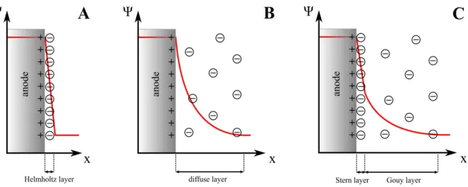
1.3 The Electrode-Electrolyte Interface

When a DC potential is applied between two electrodes immersed in an electrolyte the ions

begin to migrate to the cathode or the anode depending on their charge. According to a model

by Helmholtz

the ions in the electrolyte and the charges in the electrode form an electric

double layer with opposite charges on the electrode surface (Fig. II-4 A). This model is

analogous to a plate capacitor where the two plate electrodes are separated by a dielectric. Since

the Helmholtz model is only valid in highly concentrated electrolyte solutions and neglects ion

diffusion and thermal motion, Gouy

and Chapman

developed a theory that takes ion mobility

into account. Their model describes a diffuse double layer where the ions are distributed at a

much larger distance from the electrode (Fig. II-4 B). This theory, however, fails for high ion

concentrations or electrode potentials. Therefore, a third model was established by Stern

that

combines both theories of the Helmholtz layer and the Gouy-Chapman layer. The Stern model

describes an inner layer, the Stern layer, that consists of ions adsorbed on the charged electrode surface, and is separated from a diffuse second layer, the Gouy layer (Fig. II-4 C). It also takes into account that dissolved ions are not point charges but have a finite size and are surrounded by a hydrate shell.

Fig. II-4: (A) Helmholtz model of the double layer at the anodic electrode-electrolyte interface. The change of the electric potential Ψ with distance x from the electrode surface is schematically shown in red. (B) Gouy-Chapman model with a diffuse layer. (C) Stern model consisting of the adsorbed Stern layer and the diffuse Gouy layer.⁸²

All of these models describe the electrode-electrolyte interface for DC potentials that are below the redox potential of the electrolyte. At higher electrode potentials redox reactions occur and electrons are transferred from the cathode to an oxidant or from a reductant to the anode, causing a faradaic charge-transfer current. If there is no charge transfer between the electrode and the solution, the electrode is called ideally polarizable. Typical examples for electrodes that are ideally polarizable over a wide potential range are gold, platinum, or dropping mercury electrodes (up to 2 V).

However, polarizability of an electrode always depends on the applied potential and the electrolyte. Platinum for example is highly polarizable in NaCl solution, but becomes non-polarizable in the presence of the redox pair H

/H

. Gold is inert towards most chemicals, so that the reduction of the supporting electrolyte sets the limit for ideal polarizability.

Application of a low AC potential periodically charges and discharges the electrode surface

with positive and negative charges. This causes the ions in the solution to migrate back and

forth between the electrodes, therefore generating a non-faradaic AC current that is only caused

by ion movement. This ideal behavior can be described by a capacitor with the double layer

capacitance C

. In reality frequency dispersion occurs at solid electrodes. Therefore, the so-

called constant phase element (CPE) is commonly used to model the deviations from ideal

25 1 Impedance Spectroscopy in Aqueous Media

double layer capacitance behavior. A solution resistance R

in series with the CPE gives the complete equivalent circuit for the electrode interface and the electrolyte (Fig. II-5 A). In the corresponding Bode plot the constant impedance at high frequencies corresponds to R

(Fig.

II-5 B). The slope of |Z| at low frequencies is equal to -n in double logarithmic plots and -1 for ideal capacitive behavior. For real gold film electrodes, n takes values from 0.9 to 0.98. φ lies between -n·90° at low frequencies and 0° at high frequencies. The impedance Z

for the CPE is given by Eq. 13.

Fig. II-5: (A) Simple equivalent circuit to describe electrode and electrolyte. Rs is the solution resistance of the electrolyte and ZCPE represents the non-ideal capacitive behavior of the double layer at the electrode- electrolyte interface. (B) Corresponding schematic Bode plot. The constant impedance at high frequencies corresponds to Rs. The slope of |Z| at low frequencies is equal to -n in double logarithmic plots and -1 for ideal capacitive behavior. φ ranges from -n·90° at low frequencies and 0° at high frequencies.

Z

= 1

(jω)

·A Eq. 13

Both parameters A and n (-1 ≤ n ≤ 1) are empirical and difficult to interpret physically. When modeling the electrode-electrolyte interface n is usually close to 1 and describes a predominantly capacitive behavior. If n = 1, the impedance is that of an ideal capacitor and A is equal to the capacitance C (Fig. II-6). Other special cases for values of n are shown in Tab.

II-3.

Tab. II-3: Special cases of CPE behavior for different values of n. The parameter A corresponds to different parameters from other circuit elements depending on n.^85-86 The Warburg impedance will be addressed below.

n A

capacitance 1 C

resistance 0 R^-1

inductance -1 L^-1

Warburg impedance 0.5 (AW·√2)^-1

Fig. II-6: Capacitance dispersion effect of the CPE. In an ideal capacitor n is equal to 1 and the capacitance C is independent of the frequency. However, non-ideal capacitive behavior occurs at metal-liquid interfaces due to surfaces inhomogeneities and n usually ranges from 0.90 to 0.95. This causes a frequency dispersion of the capacitance.

The physical origin of CPE behavior at the electrode-electrolyte interface has been widely discussed in literature. Surface roughness, porosity, and varying thickness or composition of the electrode at a microscopic scale have been debated as being potential explanations for the so-called capacitance dispersion effect of a CPE.

In either case an inhomogeneous current density is present at the surface, so that the effects of solution resistance and interface capacitance are scrambled and cannot be regarded separately. Pajkossy

described these geometric inhomogeneities as being only indirectly related to the capacitance dispersion and instead attributed it to ion adsorption effects on the surface.

If charge transfer occurs, the CPE is no longer sufficient to accurately describe all processes at

the electrode surface. Instead, the Randles circuit

is commonly employed (Fig. II-7 A). It

consists of a solution resistance R

, a double layer capacitance C

, a charge-transfer resistance

R

, and a Warburg impedance Z

. As mentioned above for non-faradaic current, C

is often

replaced by a CPE.

27 1 Impedance Spectroscopy in Aqueous Media

Fig. II-7: (A) Randles circuit with solution resistance Rs, double layer capacitance Cdl, charge-transfer resistance Rct, and Warburg impedance ZW. Cdl is often replaced by a CPE. (B) Corresponding schematic Bode plot. At very low frequencies the slope of |Z| is -1/2 and φ = -45°. The plateau in the medium frequency range corresponds to Rs + Rct.

The Warburg element W is a diffusion related circuit element whose impedance Z

is given by Eq. 14 for semi-infinite linear diffusion, i.e. unrestricted diffusion to a large planar electrode.

Z

= A

·ω

- j∙A

·ω

Eq. 14

In this equation A

is the Warburg coefficient, which depends on the temperature, the surface area of the electrode, and the charge and concentration of the involved species in the electrolyte.

The Warburg impedance Z

can be recognized by a -45° phase angle at very low frequencies and a slope for |Z|(f) of -1/2 in the Bode plot (Fig. II-7 B).

The charge transfer resistance R

depends on the rate constant of the charge transfer and the concentration of the active species.

1.4 Electric Cell-Substrate Impedance Sensing (ECIS)

The theory described in chapter 1.3 has been established particularly for electrochemical

impedance spectroscopy (EIS). EIS is commonly used for the study of corrosion,

semiconductors, batteries, and electro-plating. Its basic principles have also been successfully

applied for the analysis of living cells in vitro. The first method of this kind was published by

Giaever and Keese in 1984

and later termed Electric Cell-Substrate Impedance Sensing

(ECIS). In 1991 the same authors presented an in-depth model for the analysis of a two-

dimensional cell monolayer.

This allowed the extraction of cell parameters from the impedance spectra and a detailed analysis of the morphological changes of cells grown on two coplanar gold electrodes became possible.

In ECIS measurements the impedance Z between one small working electrode (WE) and a significantly larger counter electrode (CE) is determined by application of a weak sine wave AC voltage (Fig. II-8 A). In nowadays’ commercial electrode arrays the WE has an electrode area between 5·10

cm² and 5·10

cm² and the CE is about 100 - 1000 times larger. Therefore, the voltage drop and current density at the CE can be neglected and the impedance of the overall system is almost exclusively determined by the WE. There are two general pathways for the current to cross the cell layer. At low frequencies below 10 kHz the resistive pathway around the cell body is preferred, while at higher frequencies above 10 kHz capacitive coupling through the cell membranes dominates. The resistive and capacitive components of the impedance are, however, scrambled at intermediate frequencies.

In order to model a cell layer Giaever and Keese

approximated the cells as circular disks with

a radius r and a distance h from the electrode surface (Fig. II-8 B). The current was assumed to

flow radially in the subcellular cleft underneath the cells and outward into the bulk electrolyte

through the channels between adjacent cells. Along with the presence of capacitive coupling to

the bulk electrolyte this creates a complicated electrical configuration in which the current

pathway is frequency and position dependent. There is no lumped equivalent circuit element to

describe the impedance arising from the subcellular cleft. Instead, the current flow between

electrode and cell layer was modeled using the finite element method (FEM) (Fig. II-9).

The

FEM is a numerical method where a complex problem is divided into small finite elements that

are easier to handle. Later, the equations for these elements can be combined to a complex

system to describe the entire problem.