Weekly Periodicities in Climatology

M o n d a y Tu e sd a y S u n d a y W e d n e sd a y T h u rs d a y Fr id a y S a tu rd a y M o n d a y Tu e sd a y S u n d a y W e d n e sd a y T h u rs d a y Fr id a y S a tu rd a y M o n d a y Tu e sd a y S u n d a y W e d n e sd a y T h u rs d a y Fr id a y S a tu rd a y

M o n d a y Tu e sd a y S u n d a y W e d n e sd a y T h u rs d a y Fr id a y S a tu rd a y

IAC

Institute for Atm osph e ric and Cl im ate Scie nce Sw iss Fe de ral Institute of Te ch nol ogy Z urich

Weekly Periodicities in Climatology

Master Thesis

February 2008

Authors

Peter Barmet Thomas Kuster

Supervisor

Ulrike Lohmann

Advisor

Andreas M¨ uhlbauer

I

Weekly periodicities in climatology

Master Thesis at the Institute for Atmospheric and Climate Science at “Eid- gen¨ ossische Technische Hochschule” (Federal Institute of Technology) (ETH) (IACETH). This institute is part of the Department of Environmental Sci- ences (D-UWIS).

Authors: Peter Barmet and Thomas Kuster Semester: Autumn 2007

Supervised by IAC Professor Ulrike Lohmann and PhD student Andreas M¨ uhlbauer

Thanks

We cordially thank the follwing persons:

Dominik Auf der Maur (proofreading), Caroline Baumgartner (proofread- ing), Tracy Ewen (proofreading), Reto Knutti (hints for the autocorrelation in simulations), Bettina Kuster (mental succour), Ulrike Lohmann, Massimo Merlini (statistical hints), David Masson (proofreading), Andreas M¨ uhlbauer, Hans Richner [Richner, 2007], Ariane Ritz (mental succour), Stefan Ritz (proofreading), Claudia Ryser (proofreading), Christoph Sch¨ ar (6 and 8-day- week), Marc W¨ uest (handyman)

Date and time of the L ^A TEX-run: Wednesday 27 ^th February, 2008 at 15:28

Contents

1 Introduction 1

1.1 Research that has been done on weekly cycles . . . . 2

2 Theory 5 3 Methods 9 3.1 Data Origin . . . . 9

3.2 Data Evaluation . . . . 9

3.2.1 Running Mean . . . . 10

3.2.2 Grouping by weekdays . . . . 10

3.2.3 Several Stations . . . . 10

3.2.4 Plots . . . . 11

3.2.5 Tests . . . . 11

3.2.6 Periodogram . . . . 12

3.3 Simulation . . . . 12

3.3.1 Random . . . . 12

3.3.2 Autocorrelation . . . . 12

3.3.3 Take Samples . . . . 13

3.3.4 Evaluation . . . . 14

4 Results 15 4.1 Explanatory Notes to the Results . . . . 15

4.1.1 Fundamental Assumption . . . . 15

4.1.2 Stations and their Aggregation . . . . 16

4.1.3 Faults in the Data and Data Handling . . . . 18

4.2 Particulate Matter . . . . 19

4.2.1 General Aspects of Particulate Matter Data . . . . 19

4.2.2 PM ₁₀ . . . . 19

4.2.3 PM ₁ . . . . 22

4.3 Temperature . . . . 22

IV Contents

4.3.1 Temperature Anomaly for the Time Period between

1992 and 2007 . . . . 22

4.3.2 Temperature Anomaly since 1865 . . . . 23

4.3.3 Temperature Anomaly for a 30 Year Time Period start- ing at 1960 . . . . 23

4.4 Precipitation . . . . 27

4.4.1 Precipitation in the Past for 15 Year Time Series . . . 27

4.4.2 Precipitation for Time Series of 30 Years . . . . 28

4.5 Daily Temperature Range . . . . 32

4.5.1 15 Year Steps . . . . 32

4.5.2 30 Year Steps . . . . 32

4.6 Sunshine Duration . . . . 34

4.7 Pressure . . . . 35

4.8 Four Seasons . . . . 35

4.9 Summer 2007: a Case Study . . . . 36

4.10 Simulations . . . . 44

4.10.1 Random Series . . . . 44

4.10.2 Autocorrelation . . . . 45

4.10.3 Take Samples . . . . 47

5 Discussion 49 5.1 Our Motivation and the Long Road to the Results . . . . 49

5.1.1 Assumptions and Procedures . . . . 49

5.1.2 Statistical Tests . . . . 50

5.1.3 Simulation . . . . 51

5.1.4 “6-8-Day-Test” . . . . 52

5.1.5 What else did we do . . . . 52

5.2 Discussion of the Results . . . . 52

5.2.1 Anomalies since 1865 . . . . 53

5.2.2 Summer 2007 (Case Study) . . . . 53

5.2.3 Simulation . . . . 53

5.2.4 Number of Significant Tests . . . . 54

5.3 Faults in the Data and Data Handling . . . . 55

5.4 Comparison of our Work with B¨ aumer and Vogel (2007) . . . 56

6 Conclusion and Outlook 59

Bibliography 61

A Database 65

V

B GNU R Programmes 67

B.1 gleitendesmittel.R . . . . 67 B.2 korrelation.R . . . . 68 B.3 wuerfeln.R . . . . 74 C End of the Gedanken Experiment 77

D Glossar 79

List of Figures

4.1 Distribution of the different weather conditions . . . . 16

4.2 Stations with meter above sea level . . . . 17

4.3 Temperature in August 2003, recorded at Matro . . . . 18

4.4 Weekly cycle of PM ₁₀ anomaly for the period 1998-01-01–2006- 12-31 . . . . 20

4.5 Periodogram of PM ₁₀ . . . . 21

4.6 Weekly cycle of PM ₁₀ anomaly . . . . 22

4.7 PM ₁ : Weekly cycle and Periodogram . . . . 23

4.8 Weekly cycle of temperature anomaly . . . . 24

4.9 Periodogram of temperature . . . . 25

4.10 Weekly cycles of temperature anomaly since 1865 . . . . 26

4.11 Weekly cycle of precipitation . . . . 27

4.12 Weekly cycles of precipitation for different lengths of weeks . . 28

4.13 Weekly cycles of precipitation anomaly since 1872 . . . . 29

4.14 Weekly cycle of precipitation over 30 years . . . . 31

4.15 Weekly cycle of temperature range . . . . 33

4.16 Weekly cycle of sunshine duration . . . . 34

4.17 Weekly cycle of pressure anomaly . . . . 35

4.18 Weekly cycles of precipitation by season . . . . 37

4.19 Weekly cycles of PM ₁₀ by season . . . . 38

4.20 Weekly cycles for summer 2007. Temperature and tempera- ture range. . . . 39

4.21 Weekly cycles for summer 2007. Sunshine duration and pre- cipitation. . . . 40

4.22 Weekly cycle of pressure for summer 2007 . . . . 40

4.23 Distribution of the different weather conditions per weekday during the summer . . . . 41

4.24 Weekly cycle of PM ₁₀ anomaly for summer 2007 . . . . 42

4.25 Fitting curve for air pressure . . . . 43

4.26 Histograms of 1,000 (random) simulated amplitudes for pre-

cipitation . . . . 44

VIII List of Figures

4.27 Histograms of p-values for 1,000 simulated precipitation time series . . . . 45 4.28 Weekly cycles of the first 10 simulated time series for precipi-

tation . . . . 46 4.29 Histograms of 1,000 simulated amplitudes for precipitation . . 46 4.30 Histograms of p-values for 1,000 simulated precipitation time

series with different autocorrelations . . . . 47 4.31 Weekly cycles of the first 10 simulated precipitation time series 47 4.32 Simulated time series with samples out of the original time

series. Histograms of simulated amplitudes and weekly cycles . 48 5.1 Number of siginificant tests on precipitation . . . . 55 5.2 Verifying of our calculation procedure with the German stations 57 5.3 Weekly cycles of temperature anomaly for a 6, 7 and 8-day-

week with German stations . . . . 58

A.1 Database structure . . . . 66

List of Tables

4.1 PM ₁₀ . Period: 1998-01-01 to 2006-12-31. p-values of the Kruskal-Wallistest. . . . 20 4.2 Amplitudes of weekly temperature anomalies. 15 vs. 30 year

periods . . . . 24 4.3 p-values of the Kruskal-Wallis test on precipitation anomaly.

The values are separated by time periods and stations . . . . . 30 4.4 Temperature range anomalies. Amplitudes and p-values . . . . 32 4.5 Temperature range anomalies. Amplitudes for for a 6, 7 and

8-day-week . . . . 33 4.6 Sunshine duration anomalies. Amplitudes and p-values for a

6, 7 and 8-day-week. . . . 34 4.7 Precipitation anomalies. p-values since 1870 in 30 year steps

by season. . . . 36

4.8 PM 10 . p-values by season. . . . 36

4.9 p-values for summer 2007 . . . . 42

4.10 Periodicities of the fitting curves for temperature and pressure 42

Chapter 1 Introduction

The Intergovernmental Panel on Climate Change (IPCC) report, 2007 has caused a big interest regarding global climate change in the media, politics and society. Great effort has been undertaken and is still on going to under- stand the mechanism of climate change and the anthropogenic impact on it [B¨ aumer and Vogel, 2007].

One approach for a better understanding of the anthropogenic effects on climate could be the analysis of the 7-day-periodicities in meteorological data.

Since there is no natural long-term 7-day-cycle known, one can consider the weekly anomalies in meteorological data-sets as human made. A few studies have focused on this topic (section 1.1 on the following page).

One objective of this master thesis is to check if there are similar weekly periodicities in Switzerland as B¨ aumer and Vogel (2007) found in Germany.

Therefore, precipitation, temperature and daily sunshine duration data from several measurement stations are analysed.

Questions to be answered are the following: are there any differences between stations north or south of the Alps? How do these weekly period- icities—if there are any at all—change over time? Is the signal amplitude getting stronger with increasing industrial activity and pollution? Or are these weekly differences just coincidence?

Another focus is given on the weekly regime of Particulate Matter (PM).

B¨ aumer and Vogel (2007) showed that the influence has to be at least on a

mesoscale-α (phenomenon with a range of 200–2,000 km across), due to the

fact that at mountain stations the weekly periodicity was also found. They

suppose that the connection between a microscale to a mesoscale phenomena

has to be an indirect aerosol effect.

2 Chapter 1. Introduction

1.1 Research that has been done on weekly cycles

The research on weekly cycles is not a new issue. Already in the late twenties of the last century Ashworth (1929) analysed the precipitation data from England between 1890 and 1920. He detected that there was 13% less rainfall on Sundays than on the average of all days. It was believed that the weekend reduction of smoke and hot gases from English factories was responsible for the decrease in precipitation. Referring to this, Ashworth (1933) wrote in his Nature article: “In a factory town Sunday is a day of reduced smoke pollution and concurrently Sunday is, in the long run, the day of least rainfall of any day of the week.”

In the 1960s, various authors debated whether Tuesdays, Thursdays, or Saturdays, if any day of the week, were the wettest in London, England [Schultz et al., 2007]. But no consensus was reached, in part owing to the different observing stations, time periods, and methodologies employed by these authors, as well as the lack of statistical testing [Schultz et al., 2007].

Later studies on this topic were not less contradictory. The only agree- ment between the different groups seemed to be a weekly cycle in air pol- lutants (e. g. PM with less then 10 µm in aerodynamic diameter (PM ₁₀ ) or ozone).

ˆ Dettwiller (1968) found that the precipitation on weekdays was signif- icantly higher than on weekends in five French cities. 30 years later B¨ aumer and Vogel (2007) found the contrary in Germany.

ˆ Simmonds and Kaval (1986) found a weekly cycle in Melbourne, Aus- tralia, where the precipitation on weekdays was significantly higher than on weekends.

ˆ Gordon (1994) showed through an analysis of satellite microwave sound- ing data (from the years 1979–1992) a significant but very small weekly temperature cycle for the northern hemisphere.

ˆ Simmonds and Keay (1997) found weekly cycles in temperature and precipitation in Melbourne for the period 1960–1994. They attributed these to local heat emissions.

ˆ Br¨ onimann and Neu (1997) detected weekend-weekday differences in

the near-surface ozone concentration depending on the meteorological

conditions in Switzerland.

1.1. Research that has been done on weekly cycles 3

ˆ Cerveny and Balling Jr. (1998) identified weekly cycles of precipita- tion and tropical cyclone maximum wind speed over the North-West Atlantic region and explained this with the help of an air pollution in- dex that also showed a weekly cycle. Furthermore they detected that the difference of day and night wind speed in tropical cyclones reveals a weekly periodicity.

ˆ Beaney and Gough (2002) found weekend-weekday differences of ozone and temperature in Toronto. As they did not find these difference in the data of a remote station they concluded that it has to be a local phenomenon.

ˆ Marr and Harley (2002) detected weekend-weekday differences of ozone, VOCs and NOx (in 1980–1999) at several stations in California.

ˆ Cerveny and Coakley (2002) identified a weekly cycle of CO ₂ at Mauna Loa, Hawaii. However at the South Pole they did not find a 7-day cycle.

ˆ Delene and Ogren (2002) and Jin et al. found weekly periodicities of aerosol optical properties at different locations in North-America.

ˆ Beirle et al. (2003) analysed satellite data and found significant weekly cycles of tropospheric NO ₂ over many industrialised regions.

ˆ Forster and Solomon (2003) detected a weekend effect in the daily tem- perature range in different regions.

ˆ Tsai (2005) found differences of the visibility and the PM 10 concentra- tion between weekdays and weekends in Taiwan.

ˆ Shutters (2006) reported weekly cycles of various chemical variables and of wind speed in Phoenix, Arizona.

ˆ Gong et al. (2006) found increasing weekly cycles in various meteoro- logical parameters (e. g. temperature and precipitation) in China.

ˆ B¨ aumer and Vogel (2007) showed that climatological variables in Ger- many have an unexpected weekly distinction. They chose data from 1991 to 2005 from the “Deutscher Wetterdienst” (German Weather Service) (DWD)

In contrast, other studies found no statistically significant signal between weekday and weekend precipitation. For example:

ˆ Cehak (1982) in Vienna, Austria

4 Chapter 1. Introduction

ˆ Horsley and Diebolt (1995) in five Midwestern US cities

ˆ De Lisi et al. (2001) along the Northeast Corridor

ˆ Wilby and Tomlinson (2000) at 92 stations in the United Kingdom Schultz et al. (2007) state that there is no significant weekly precipitation cycle at all: “Daily precipitation records for 219 surface observing stations in the United States for the 42-year period 1951–1992 are investigated for weekly cycles in precipitation. Results indicate that neither the occurrence nor amount of precipitation significantly depends upon the day of the week.”

They confirm the result of De Lisi et al. (2001) who did not find a significant weekly precipitation cycle along the Northeast Corridor. They even question the results of a study with the satellite derived precipitation estimates by Cerveny and Balling Jr. (1998) due to “the potential problems in estimating precipitation from Microwave Sounding Unit (MSU) data [Spencer, 1993], as well as questionable causal links between their data sets”.

This thesis is organised as follows: Chapter 2 focuses on a few hypothe- sised theories, that try to explain how a weekly cycle could come into being.

Chapter 3 focuses on the methods applied hereinafter. In Chapter 4 the re-

sults will be presented and discussed in Chapter 5. Chapter 6 is reserved for

a short conclusion and an outlook.

Chapter 2 Theory

Probably the oldest scientific theory about precipitation manipulation by humans is the inducement of convection. Referring to this Ashworth (1929) writes: “In a confined manufacturing area, such as the town of Rochdale, with a large number of factories burning quantities of coal of the order of 500 to 10,000 tons a day, it is not unlikely that the volume of heated gases which rises is sufficient to give that uplift to the atmosphere which is required to provoke an increase of rain.” At that time it was already known that a slight uplift to the air—such as caused by the passage of the wind over a small elevation of the land in a flat country—augments the precipitation. In this context Ashworth (1929) states: “This effect on an uplift to the air may be looked for over a collection of mill chimneys from which a considerable upward current of hot gases issues for a third to a half of the 24 hours.”

He also assumes that there might be another possible effect which triggers precipitation: “There is also the probability that the fine flue dust ejected by the draught up the chimney may supply an abundance of the nuclei which promote the formation of rain [. . . ].”

In cloud physics, the hypothesis—by supplying additional cloud conden- sation and ice nuclei, pollution downwind from urban centres would increase precipitation occurrence, precipitation amount, or both—has been supported for a long time. Research since the late 1980s, however, suggests that anthro- pogenic aerosols may decrease precipitation occurrence and amount because pollution particles cause the same amount of cloud water to be distributed among more droplets, hence the droplets are smaller and less likely to grow to precipitation-sized particles. The hypothesised result is that precipitation is less likely to occur [Schultz et al., 2007]. B¨ aumer and Vogel (2007) conclude:

“Since also cloud amount and precipitation are modified in the course of a

week, we suppose that the indirect aerosol effects on cloud properties and

precipitation play an important role. The prevalent ideas about coherences

6 Chapter 2. Theory

between an increase in aerosol particle number, an increase in cloud droplets number but a decrease of their radii, and a following decrease of precipitation but longer cloud lifetimes, is not reflected by our results.”

Gong et al. (2007) hypothesised that the changes in the atmospheric circulation may be triggered by the accumulation of PM 10 through diabatic heating of the lower troposphere. During the early part of a week the an- thropogenic aerosols are gradually accumulated in the lower troposphere.

Around midweek, the accumulated aerosols could induce radiative heating, likely destabilising the middle to lower troposphere and generating anoma- lously vertical air motion and thus resulting in stronger winds. The result- ing circulation could promote ventilation to reduce aerosol concentrations in the boundary layer during the later part of the week. Corresponding to this cycle in anthropogenic aerosols, the frequency of precipitation, partic- ularly the light rain events, tends to be suppressed around midweek days through indirect aerosol effects. This is consistent with the observed anthro- pogenic weather cycles, e. g. more (less) solar radiation near surface, higher (lower) maximum temperature, larger (smaller) diurnal temperature range, and fewer (more) precipitation events in midweek days (on weekends) [Gong et al., 2007].

Not only the amount of aerosols influence the meteorology. It also de- pends on whether these aerosols can act as Cloud Condensation Nuclei (CCN) and on their size distribution:

ˆ Dusek et al. (2006) detected that aerosol size distribution, particularly that of fine aerosols, plays a significant role in the nucleation of cloud particles which is one of the primary mechanisms of indirect aerosol effects. Furthermore they found that the size matters more than chem- istry for the cloud-nucleating ability of aerosol particles.

ˆ An experimental study by Yin et al. (2000) investigated the effect of gi- ant CCN on the development of precipitation in mixed-phase convective clouds. Their results showed that the strongest effects of introducing giant CCN occur when the background concentration of small nuclei is high, as it is in continental clouds. Under these conditions, the coa- lescence between water drops is enhanced due to the inclusion of giant CCN. This leads to an early development of large drops in the lower parts of the clouds. In maritime clouds, where the background concen- tration of small nuclei is low, the effect of the giant CCN is smaller and the development of precipitation is dominated by the droplets formed on large nuclei.

These results show that it is not trivial to determine the important pa-

7

rameters that have to be analysed in the following. Due to the fact that only

PM has been analysed systematically over a longer time period and a certain

range, the data used for the computations in Results Chapter, Section 4.2

Particulate Matter, on page 19 are PM ₁₀ and PM with less then 1 µm in

aerodynamic diameter (PM 1 ).

Chapter 3 Methods

3.1 Data Origin

Switzerland has an automatic meteorological network since 1978. From some stations longer time series are available [ANETZ, 1980; Zellweger, 1983]. All meteorological data are provided by the Federal Office of Meteorology and Climatology (MeteoSwiss). PM is measured by the “Nationales Beobach- tungsnetz f¨ ur Luftfremdstoffe” (National Observation Network for Foreign Air Contaminants) (NABEL) and the data are provided by the “Bundes- amt f¨ ur Umwelt” (Federal Office for the Environment) (BAFU) and the

“Eidgen¨ ossische Material Pr¨ ufungsanstalt” (Material Science & Technology) (Empa).

The data for Germany are available from the DWD.

In this work only daily values are considered which are mostly computed from ten minutes values.

To facilitate the handling, all measured values used in the computations are stored in a database (details in Appendix A on page 65).

3.2 Data Evaluation

Climatological variables have different fluctuations caused by diurnal and seasonal cycles and diverse weather conditions.

For the analysis of a 7-day cycle, it is advisable to filter these cycles, pri-

marily diurnal and seasonal ones. Considering only daily values, the diurnal

cycle does not matter anymore.

10 Chapter 3. Methods

3.2.1 Running Mean

A simple method to filter out these fluctuations is to compute the deviation to a running mean.

This deviation (δ d ) is computed as follows:

δ _d = v _d − 1

∆

d+

X

i=d−

2

v _i (3.1)

The given measured value at day d is given as v _d , then the mean of the ∆ days—which has to be odd—around the day d are subtracted (Equation 3.1).

B¨ aumer and Vogel (2007) set ∆ to 31 days.

In GNU R (R) this is realised with the function gleitendesmittel.R (Appendix, Section B.1 on page 67). The result is a new time series, which contains the daily deviation from the running mean and is called the “time series of deviation” (δ).

3.2.2 Grouping by weekdays

The “time series of deviation” (δ) can be grouped by weekdays. This gives 7 time series (δ _weekday

), one for each weekday (Equation 3.2).

δ _Monday

= {δ _d |d is Monday}

δ _Tuesday

= {δ _d |d is Tuesday}

.. .

δ _Sunday

= {δ _d |d is Sunday} (3.2)

Calculating the mean of each group provides the deviation for every weekday (¯ δ _weekday ) (Equation 3.3).

δ ¯ _weekday = 1

w _end − w _begin + 1

w

X

w=w

δ _weekday

(3.3)

It is also possible to group the measured values directly by weekdays.

The result is a distribution in both cases.

3.2.3 Several Stations

There are two possibilities to compute ¯ δ _weekday if there are data available from

more than one station.

3.2. Data Evaluation 11 1. Group directly by weekday, as described in 3.2.2 on the preceding page 2. First aggregate the data for each single day and then group them by

weekday

The number of the δ _weekday is higher in the first case (by a factor of the number of stations).

3.2.4 Plots

If the time dependence is neglected, δ weekday can be considered as a distribu- tion, so it is possible to calculate e. g. the standard deviation and standard error and plot the weekly cycle with errorbars.

3.2.5 Tests

With δ _weekday as a distribution it is possible to run a statistical test, e. g.

Wilcoxon test one sided, of the maximum mean against the one with the minimum—this corresponds to the amplitude of the weekly cycle. Due to the fact that more than two groups exist (equal to the number of weekdays) an analysis of variance might be more appropriate, e. g., with the Kruskal- Wallis test.

If a time series (δ or v) of a station correlates with another one, they are not independent and therefore to group them directly by weekday (Sec- tion 3.2.3 on the facing page item 1) is not correct for the tests mentioned previously. To check whether the time series from the different stations cor- relate with each other, they can be tested against each other. It is important to test only the filtered time series. In R this can be done with the func- tion cor.test and is realised in the program korrelation.R, Appendix, Section B.2 on page 68.

Another simple way to compare whether or not there is a weekly cycle, is to assume a 6-day-week and a 8-day-week. To distinguish between the

“weeks” the following names for the weekdays are chosen:

6-day-week Jeroboam, Rehoboam, Methuselah, Shalmanazar, Balthazar and Nebuchadnezzar ¹

7-day-week Monday, Tuesday, Wednesday, Thursday, Friday, Saturday and Sunday ²

1 Names of wine bottles

2 It is difficult to explain where these names come from

12 Chapter 3. Methods

8-day-week Bo, Hamm, Slink, Potato, Woody, Sarge, Etch and Lenny ³

3.2.6 Periodogram

A periodogram is an estimate of the spectral density of a signal. It allows certain frequencies in a time series to be detected—unless there are any at all.

A weekly cycle in the daily measured values provides a peak at the frequency of ¹ ₇ and at the multiples of it.

3.3 Simulation

Another plausibility check can be done by comparing the results with a ran- dom process. Different methods are used to create a random sequence. The target of all these methods is to create a new time series with the same length and the same characteristic as the original one but without a possible weekly cycle. The simulation can be based on the original time series with the measured values or on the “time series of deviation”.

3.3.1 Random

There are two ways to create a new absolutely random series with the same length and standard deviation as the original time series.

ˆ A random order of the time series

ˆ A distribution with the same standard deviation and length as the time series

3.3.2 Autocorrelation

The time series has an autocorrelation, because a meteorological measured value often depends on the preceding value. The new time series (a k ) is computed as follows: the first entry is set to the mean of the original time series ¯ δ. The next entry is then computed from the entry before and a random

3 Names of Debian releases

3.3. Simulation 13 part (equation 3.4).

a ₁ = ¯ δ

a 2 = a 1 · % + (1 − %) · r 1

a ₃ = a ₂ · % + (1 − %) · r ₂ .. .

a _n = a n−1 · % + (1 − %) · r n−1 (3.4) r i is a random number from a distribution with the same standard deviation as the original time series and % is the autocorrelation of it. The autocorre- lation % is the estimated measure of association of the time series with itself shifted by one day, which corresponds to one entry. In R this is realised with the function cor.test as follows:

1 rho <- cor . test ( t i m e s e r i e [1:( l e n g t h ( t i m e s e r i e ) -1) ] , t i m e s e r i e [2:( l e n g t h ( t i m e s e r i e ) ) ]) $ e s t i m a t e

Setting the autocorrelation to a arbitrary value is useful for comparison (e. g. 0 and 0.9).

It is not advisable to do these simulations with the measured values be- cause they have a seasonal cycle.

3.3.3 Take Samples

The time series created in Section 3.3.2 on the preceding page could lack a feature describing the original time series. Another approach is to create a new time series (s k ) with samples from the original time series, which then exhibits the same length as the week. The procedure is shown in Equa- tion 3.5:

First week of the new time series



 

 

 

 

s ₁ = δ _r

₊₁ s ₂ = δ _r

₊₂

.. .

s _w = δ _r

_+w

Second week of the new time series



 

 

 

 

s w+1 = δ r

+1

s _w+2 = δ _r

₊₂ .. .

s _w+w = δ _r

_+w Third week of the new time series

( s 2w+1 = δ r

+1

.. . (3.5)

14 Chapter 3. Methods

r _i is a random number between 0 and the length of the time series minus the length of the week and w is the length of the week.

3.3.4 Evaluation

The weekdays are matched to each of these new time series. The first entry in the time series is Monday (Jeroboam or Bo depending on the length of the week) the second Tuesday (Rehoboam or Hamm) and so on.

To receive the amplitude of the average weekly cycle one has to subtract the weekday with the minimum mean value from the one with the maxi- mum mean value. Repetitions of this procedure allow a histogram of the amplitudes to be made.

Storing the mean of each weekday from a few runs allows the simulated weekly cycle to be compared with the original one.

To compare the different tests presented in Section 3.2.5 on page 11, the same procedure as for the amplitude is used with the p-values of each test.

Thus one can make a histogram of the p-values.

Chapter 4 Results

4.1 Explanatory Notes to the Results

4.1.1 Fundamental Assumption

First of all—before the results are computed—one has to make sure that the assumption “there is no natural seven-day cycle” is true. Therefore it is appropriate to have a look at the “Witterungslagen nach Sch¨ uepp”

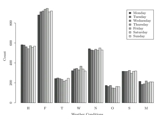
(‘synoptical weather classification by Sch¨ uepp’). This is a classification based only on dynamics. It classifies the weather conditions in 8 main-groups which then subsequently are grouped in 5 subgroups. In this Chapter, for practical reasons, only the 8 main-classes are considered, which are:

ˆ “Hochdrucklage” (high pressure condition) (H)

ˆ “Flache (mittlere) Druckverteilung” (weather conditions with a flat pressure distribution) (F)

ˆ “Tiefdrucklage”(low pressure condition) (T)

ˆ “Weststr¨ omung” (west stream) (W)

ˆ “Nordstr¨ omung” (north stream) (N)

ˆ “Oststr¨ omung” (east stream) (O)

ˆ “S¨ udstr¨ omung” (south stream) (S)

ˆ “Mischlage” (M)

16 Chapter 4. Results

Monday Tuesday Wednesday

Sunday Saturday Friday Thursday

H F T W N O S M

0 20 0 40 0 60 0 80 0

Weather Conditions

Co un t

Figure 4.1: Distribution of the different weather conditions (since 1945) per weekday

H, F, T are called ‘convective conditions’ and W, N, O, S are called ‘advective conditions’. They all refer to the situation at the 500 hPa-layer, while M can have either strong winds on the ground or higher up as a jetsteam.

The count of the several “Witterungslagen” per weekday since 1945 shows that there is no dynamical 7-day cycle (Figure 4.1) so that the assumption from above is consequently correct.

4.1.2 Stations and their Aggregation

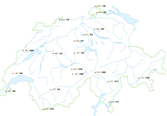
In the following Chapters the meteorological-data are used from: Bargen (SH), Bi` ere, Binningen, Col du Grand St-Bernard, Egolzwil, Gen` eve, La Br´ evine, Lugano, M¨ annlichen, Matro, Mosen, Passo del S. Gottardo, Schaffhausen, Sch¨ upfheim, Segl-Maria, Sion, Zollikofen and Z¨ urich (Figure 4.2 on the next page). This 18 CLIMAP-stations provide temperature values since 1864.

The PM ₁₀ values are derived from NABEL-stations which are located in:

Basel, Bern, Lugano and Z¨ urich. The measurements go back to the year 1998. For the sommer 2007 the station Jungfraujoch is also available.

The availability of the PM ₁ -data is of a shorter time series, namely since

4.1. Explanatory Notes to the Results 17

Figure 4.2: Stations with meter above sea level: Bargen (SH) (BAR),

Bi` ere (BIR), Binningen (Basel) (BAS), Col du Grand St-Bernard (GSB),

Egolzwil (EGO), Gen` eve-Observatoire (GEO), Jungfraujoch (JUN), La

Br´ evine (BRL), Lugano (LUG), M¨ annlichen (MAE), Matro (MTR), Mosen

(MOA), Passo del S. Gottardo (GOH), Schaffhausen (SHA), Sch¨ upfheim

(SPF), Segl-Maria (SIA), Sion (ION), Zollikofen (Bern) (BER) and Z¨ urich

(SMA)

18 Chapter 4. Results

510152025303540

Time

DailyTemperatureMean[°C]

Aug 01 Aug 06 Aug 11 Aug 16 Aug 21 Aug 26 Aug 31

(a) Daily values

251020501002005002000

Time

Temperature[°C]

Aug 01 Aug 06 Aug 11 Aug 16 Aug 21 Aug 26 Aug 31

(b) 10 minutes values

Figure 4.3: Temperature 2 m above ground in August 2003, recorded at Matro.

2003. The geographical coverage is also smaller and consists of only three sta- tions: Basel, Bern and Lugano. Hereinafter the PM 1 -values between March 2003 and December 2006 are analysed.

Usually the data of these stations are aggregated and the mean over all stations is used for further calculations. This allows results which reflect the entire area of Switzerland to be generated. This might smooth a possible local weekly course. To be on the safe side—regarding this “aggregation problem”—each of the 18 stations is always considered and also separately tested.

4.1.3 Faults in the Data and Data Handling

All meteorological data are derived from the Java application to get data from MeteoSwiss (CLIMAP). Some of them can not be true. E. g. the temperature series of Matro contains some very high daily temperature values (exceeding 35 ° C). They are based on wrong 10 minutes values with a temperature of 3108.2 ° C (Figure 4.3). Therefore all extreme values in precipitation, daily mean temperature, daily minimum and maximum temperature had had to be manually checked for plausibility check: all values that exceed the Swiss all-time record have been dropped and those which are in the range of it have been carefully analysed. Another method to detect wrong values is to look for the outliers in the “time series of deviation”.

Even by removing the sparse existing incorrect data, the results do not change significantly. Only in the precipitation results, it does observably diminish the errorbars.

When a station contains more than 20% unavailable data in a considered

4.2. Particulate Matter 19 period, the station drops out automatically for this period.

As long as not stated otherwise, the analysed time series refer to the devi- ation from the 31-day running mean. This allows, e. g., to make a correlation test between the stations without testing the seasonal cycle. The resulting smaller standard deviation leads to narrower errorbars and the statistical tests reveal better results (due to the filtered time series).

4.2 Particulate Matter

B¨ aumer and Vogel (2007) hypothesised that the indirect aerosol effect is responsible for weekly cycles in meteorological data. Therefore PM ₁₀ and PM ₁ are analysed first.

4.2.1 General Aspects of Particulate Matter Data

Since there are no PM ₁₀ values available before 1998, a comparison with ear- lier periods is not possible. Nevertheless—thanks to the correlation between suspended matter and PM ₁₀ —there are facilities to convert one into the other. Based on the suspended matter measurements the BAFU computed the PM ₁₀ values back until 1988. In this longer time series one can recognise a clear decreasing trend over the last 20 years, especially in the cities. The BAFU reckons also that the maximum PM ₁₀ -pollution was around 1970. For this reason the further analysis of longer meteorological time series (in the fol- lowing Sections) often consider the period between 1960 and 1990 [BUWAL, 2005].

One assumes that the small particles of the PM ₁₀ -fraction have more influence on clouds than the bigger ones (Chapter 2 Theory on page 6).

4.2.2 PM ₁₀

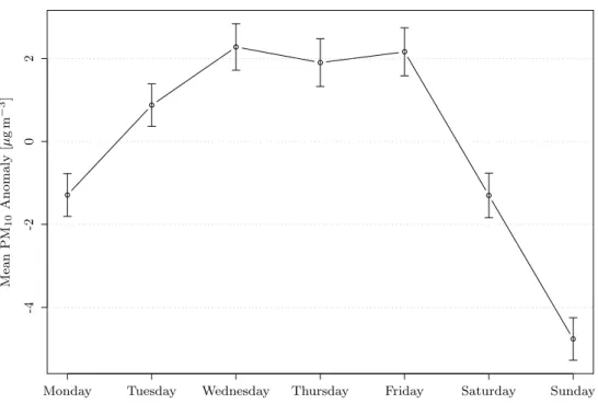
Figure 4.4 on the next page shows the weekly course of PM ₁₀ . Data since January 1998 have been evaluated from the five NABEL-stations mentioned before. The range between the maximum on Wednesday and the minimum on Sunday is almost 7 µg m ⁻³ .

The Kruskal-Wallis test over the seven weekdays (on the average over all

stations) reveals a significance at very high level with a p-value of 6 · 10 ⁻²⁹ .

This means that there is a weekly cycle which can hardly be coincidence. In

fact every single station shows a highly significant (α = 0.3%) weekly cycle

(Table 4.1 on the following page).

20 Chapter 4. Results

Monday Tuesday Wednesday Thursday Friday Saturday Sunday

-4 -2 0 2

Mean P M

Anom aly [ µ g m

]

Figure 4.4: Weekly cycle of PM ₁₀ anomaly averaged over the following sta- tions: Basel, Bern, Lugano, Z¨ urich. Period: 1998-01-01 to 2006-12-31. Er- rorbars: ±1 standard error.

Table 4.1: PM ₁₀ . Period: 1998-01-01 to 2006-12-31. p-values of the Kruskal- Wallistest.

Station p-value

Basel 2.30·10 ⁻¹⁰

Bern 1.09·10 ⁻⁶⁶

Lugano 3.98·10 ⁻¹¹

Z¨ urich 1.77·10 ⁻¹⁹

Average 6.00·10 ⁻²⁹

4.2. Particulate Matter 21

0.0 0.1 0.2 0.3 0.4 0.5

2 5 10 20 50 10 0 20 0 50 0 10 00

Frequency [d

]

Sp ec trum

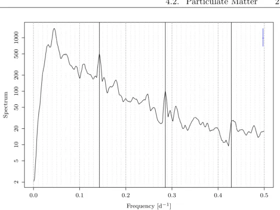
Figure 4.5: Smoothed periodogram of PM 10 . Bandwidth=0.00243. Period:

1998-01-01 to 2006-12-31.

The first peak is at ₃₁ ¹ d ⁻¹ because smaller frequencies are filtered out through a 31-day running mean.

Peaks at ¹ ₇ d ⁻¹ and the multiples of it point to a 7-day cycle in PM ₁₀ .

“The cross emblem in the upper right corner of the plot represents the band- width of the smoother (cross-piece) and the upper and lower bounds of a pointwise 95% confidence interval for the spectral density about the plotted curve (vertical line of the cross)” [Smith, 1999, page 49].

The Fourier Analysis on the time series of the PM ₁₀ deviation from the running mean provides a periodogram which yields a clear peak at ¹ ₇ d ⁻¹ and the multiples of it (vertical black lines in Figure 4.5) that in turn marks the 7-day cycle.

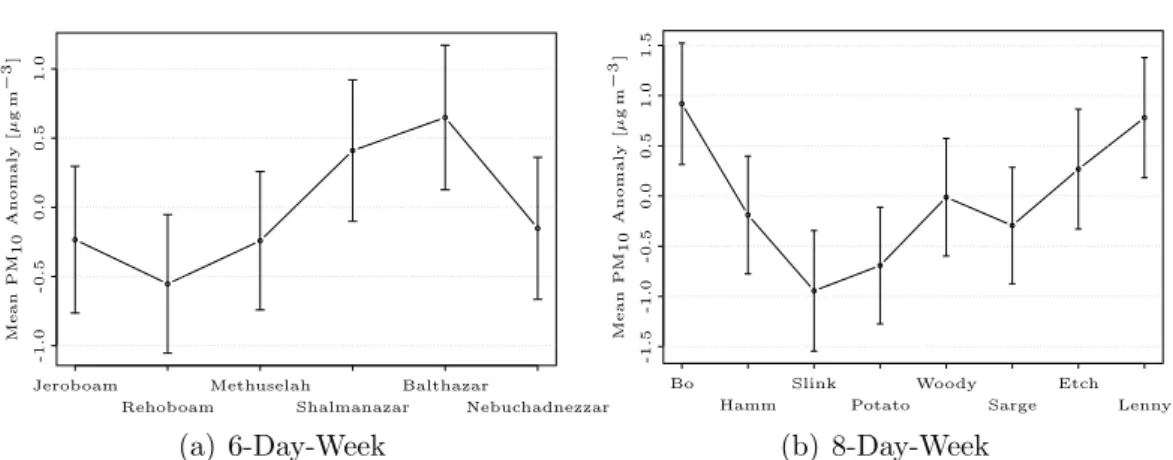
Assuming a 6 or an 8-day-week the amplitudes become at least 3 times

smaller. The range for an 8-day-week is almost 1.9 µg m ⁻³ while for a 6-

day-week it is only around 1.1 µg m ⁻³ (Figure 4.6 on the following page).

22 Chapter 4. Results

Jeroboam Rehoboam

Methuselah Shalmanazar

Balthazar

Nebuchadnezzar

-1.0-0.50.00.51.0

MeanPM10Anomaly[µgm−3]

(a) 6-Day-Week

Bo Hamm

Slink Potato

Woody Sarge

Etch Lenny

-1.5-1.0-0.50.00.51.01.5

MeanPM10Anomaly[µgm−3]

(b) 8-Day-Week

Figure 4.6: Weekly cycle of PM ₁₀ anomaly averaged over the following sta- tions: Basel, Bern, Lugano, Z¨ urich. Period: 1998-01-01 to 2006-12-31. Er- rorbars: ±1 standard error. Note that the range of the ordinate varies.

4.2.3 PM ₁

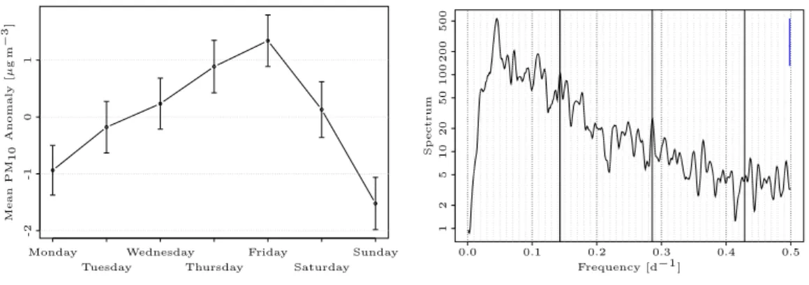
The weekly course of PM ₁ has an amplitude of about 2.9 µg m ⁻³ . Applying the Kruskal-Wallis test on it, reveals a high significance (α = 0.3%) with a p-value of 2.165e-06. The minimum falls on Sunday. From then on there is a constant ascent to the maximum on Friday (Figure 4.7(a) on the next page).

The Fourier Analysis on the PM ₁ -values (Figure 4.7(b) on the facing page) provides a periodogram which yields a clear peak at ¹ ₇ d ⁻¹ and the multiples of it. This underlines the result from the Kruskal-Wallis test, which show that the PM ₁ weekly course is statistically significant.

The analysis of this result, by assuming a 6 and an 8-day-week (and by doing preceding procedure again), reveals apparent smaller amplitudes as for the regular week. For a 6-day-week it is about 1.1 µg m ⁻³ and for the 8-day-week it is 0.7 µg m ⁻³ . In both cases the Kruskal-Wallis test reveals no significance: neither for the shortened week (p-value is 0.64) nor for the extended week (p-value is 0.92)

4.3 Temperature

4.3.1 Temperature Anomaly for the Time Period be- tween 1992 and 2007

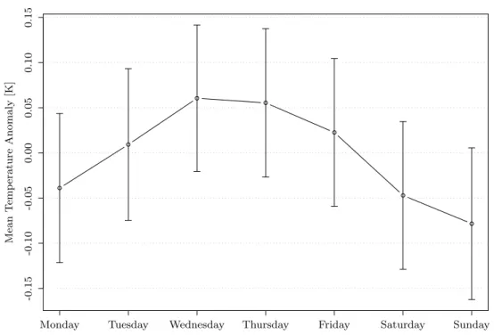
The analysis of the temperature anomaly for the 15 years from 1992 to

2007 reveals no significance: even if there is a small amplitude of 0.15 K

4.3. Temperature 23

Monday Tuesday

Wednesday Thursday

Friday Saturday

Sunday

-2-101

MeanPM10Anomaly[µgm−3]

(a) Weekly cycle of PM ₁ anomaly. Error- bars ±1 standard error.

0.0 0.1 0.2 0.3 0.4 0.5

125102050100200500

Frequency [d−1 ]

Spectrum

(b) Smoothed Periodogram with band- width=0.00176.

Figure 4.7: PM ₁ for following stations: Basel, Bern, Lugano. Period: 2003- 01-01 to 2006-12-31

between the maximum on Wednesday and the minimum on Sunday (Fig- ure 4.8 on the next page), the Kruskal-Wallis test reveals a p-value of 0.805 which means that this weekly course is not significant. Even when applying this test to each of the 18 stations, none provides a significant weekly cycle in temperature—not even at the 10% level, all p-values are greater then 0.1.

This result can be confirmed by applying the “6-8-week-day-test” and with several simulations (Section 4.10 on page 44).

Examining the periodogram of the temperature deviation (Figure 4.9 on page 25) no peak can be detected at ¹ ₇ d ⁻¹ and its multiples. Therefore it seems to be quite coincidental to assume a 7-day-cycle in temperature.

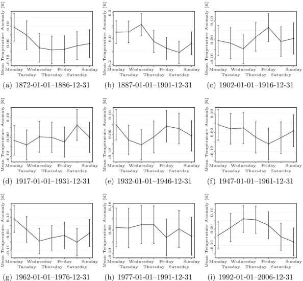
4.3.2 Temperature Anomaly since 1865

Considering the plots since 1865 (Figure 4.10 on page 26) one can not recog- nise a clear weekly trend which lasts for more than 30 years. The amplitudes however are—during the considered 140 years—more or less around 0.12 K.

4.3.3 Temperature Anomaly for a 30 Year Time Period starting at 1960

Considering the time period with the highest PM ₁₀ air pollution (Section 4.2

on page 19) the weekly course reveals a maximum on Monday and a mini-

mum on Sunday. The amplitude between the two is 0.07 K. It is remarkable

that, by doubling the considered time period, the amplitude almost bisects

(Table 4.2 on the following page).

24 Chapter 4. Results

Monday Tuesday Wednesday Thursday Friday Saturday Sunday

-0. 15 -0. 10 -0. 05 0.0 0 0.0 5 0.1 0 0.1 5

Mean T emp era ture Anoma ly [K]

Figure 4.8: Weekly cycle of temperature (2 m above ground) anomaly av- eraged over all stations. Period: 1992-01-01 to 2006-12-31. Errorbars: ±1 standard error.

Table 4.2: Amplitudes of weekly temperature anomalies. 15 vs. 30 year periods

15 years amplitude amplitude 30 years

1872–1886 0.132 0.12 1870–1899

1887–1901 0.218

1902–1916 0.113 0.02 1900–1929

1917–1931 0.098

1932–1946 0.103 0.07 1930–1959

1947–1961 0.102

1962–1976 0.141 0.07 1960–1989

1977–1991 0.055 1992–2006 0.139

average 0.122 0.072 average

4.3. Temperature 25

0.0 0.1 0.2 0.3 0.4 0.5

0.1 0.2 0.5 1.0 2.0 5.0 10 .0 20 .0 50 .0

Frequency [d

]

Sp ec trum

Figure 4.9: Smoothed periodogram of temperature (2 m above ground).

Bandwidth=0.00146. Period: 1992-01-01 to 2006-12-31

The high peak at ₃₁ ¹ d ⁻¹ is because smaller frequencies are filtered out through a 31-day running mean. The very first peak at ₃₆₅ ¹ d ⁻¹ ≈ 0.003 d ⁻¹ reflects the not perfectly filtered seasonal cycle.

No peak can be detected at ¹ ₇ d ⁻¹ and its multiples.

“The cross emblem in the upper right corner of the plot represents the band-

width of the smoother (cross-piece) and the upper and lower bounds of a

pointwise 95% confidence interval for the spectral density about the plotted

curve (vertical line of the cross)” [Smith, 1999, page 49].

26 Chapter 4. Results

0.15-0.05-0.100.000.10

Monday

MeanTemperatureAnomaly[K]

Wednesday Thursday

Friday Sunday

Tuesday Saturday

0.05

(a) 1872-01-01–1886-12-31

Wednesday Thursday

Friday Saturday

Sunday

-0.20.2

MeanTemperatureAnomaly[K]

Tuesday Monday

0.0-0.10.1

(b) 1887-01-01–1901-12-31

Monday

Tuesday Thursday

Friday Saturday

Sunday

-0.10-0.050.000.050.100.15MeanTemperatureAnomaly[K]

Wednesday

(c) 1902-01-01–1916-12-31

Tuesday Thursday

Friday Saturday

Sunday

-0.10-0.050.000.050.100.15

MeanTemperatureAnomaly[K]

Monday Wednesday

(d) 1917-01-01–1931-12-31

Monday Tuesday

Wednesday Thursday

Friday Saturday

Sunday

-0.10-0.050.000.050.10

MeanTemperatureAnomaly[K]

(e) 1932-01-01–1946-12-31

Monday Tuesday

Wednesday

Thursday Saturday

Sunday

-0.15-0.10-0.050.000.050.10MeanTemperatureAnomaly[K]

Friday

(f) 1947-01-01–1961-12-31

Monday Tuesday

Wednesday Thursday

Friday Saturday

Sunday

-0.10-0.050.000.050.100.15

MeanTemperatureAnomaly[K]

(g) 1962-01-01–1976-12-31

Monday Tuesday

Wednesday Thursday

Friday Saturday

Sunday

-0.10-0.050.000.050.10

MeanTemperatureAnomaly[K]

(h) 1977-01-01–1991-12-31

Monday Tuesday

Wednesday Thursday

Friday Saturday

Sunday

-0.15-0.10-0.050.000.050.100.15MeanTemperatureAnomaly[K]

(i) 1992-01-01–2006-12-31

Figure 4.10: Weekly cycles of temperature anomaly since 1865 in 15 year

time steps. Average over all stations. Errorbars: ±1 standard error. Note

that the range of the ordinate varies from period to period.

4.4. Precipitation 27

Monday Tuesday Wednesday Thursday Friday Saturday Sunday

-0. 3 -0. 2 -0. 1 0.0 0.1 0.2 0.3

Mean P recipi tatio n Anom aly [m m]

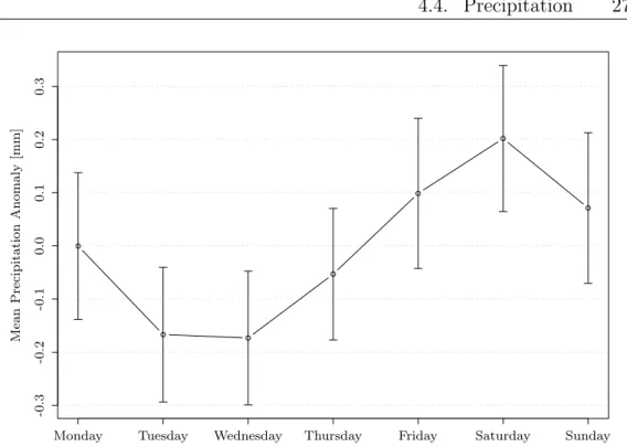
Figure 4.11: Weekly cycle of daily precipitation (5:40 to 5:40 UTC) anomaly averaged over all stations. Period: 1992-01-01 to 2006-12-31. Errorbars: ±1 standard error.

4.4 Precipitation

The weekly course in the mean precipitation anomaly reveals a minimum on Wednesday and a maximum on Saturday which leads to an amplitude of more than 4 mm (Figure 4.11). According to the errorbars one could assume that this cycle could be significant: the errorbars of Wednesday and those of Sunday do not overlap. But the Kruskal-Wallis test reveals another result:

the aberrations from the medians are not significant.

The second test—with the assumed 6 and 8-day-weeks—reveals similar amplitudes as the regular week and the errorbars of the maximum and the minimum do not overlap either (Figure 4.12 on the following page).

Moreover with an appropriate model one can point out that such a weekly course—with an amplitude in the same range—can simply be simulated (Sec- tion 4.10 on page 44).

4.4.1 Precipitation in the Past for 15 Year Time Series

Going back into the past—in 15 year time steps—the maximum and the

minimum seem to vary arbitrarily. The weekly anomaly range in precipita-

28 Chapter 4. Results

Jeroboam Methuselah

Shalmanazar Balthazar

Nebuchadnezzar

-0.2-0.10.00.10.20.3

MeanPrecipitationAnomaly[mm]

Rehoboam

(a) 6-Day-Week

Bo Hamm

Slink Potato

Woody Sarge

Etch Lenny

-0.2-0.10.00.10.20.3

MeanPrecipitationAnomaly[mm]

(b) 8-Day-Week

Figure 4.12: Weekly cycles of daily precipitation (5:40 to 5:40 UTC) anomaly averaged over all stations for different lengths of weeks. Period: 1992-01-01 to 2006-12-31. Errorbars: ±1 standard error. Note that the range of the ordinate varies.

tion between 1992 and 2006 is almost 0.4 mm. Compared to the past this is remarkably high. Only in the period between 1872 and 1886 does the amplitude yield a similar range (Figure 4.13 on the facing page).

Nevertheless the Kruskal-Wallis test does not reveal a significance for the average over all stations nor for a single one. This applies to all analysed time periods (Table 4.3 on page 30).

4.4.2 Precipitation for Time Series of 30 Years

The analysis of 30 year time series does not reveal large differences compared

to those of 15 years. Every timestep provides a graph with a divers look. The

one between 1960 and 1990—which corresponds to the time period with the

highest PM ₁₀ pollution—has an amplidude of a little bit more than 1 mm

(Figure 4.14 on page 31). All errorbars overlap with each other and the

Kruskal-Wallis test does not reveal a significance. Compared to the 6 and

8-day-week the amplitudes are all in the same range—around 1 mm: the

amplitude of the 8-day-week exceeds the regular one while the 6-day-week

does not.

4.4. Precipitation 29

Monday

Tuesday Thursday

Friday Saturday

Sunday

-0.3-0.2-0.10.00.10.20.3MeanPrecipitationAnomaly[mm]

Wednesday

(a) 1872-01-01–1886-12-31

Monday Tuesday

Wednesday Thursday

Friday Saturday

Sunday

-0.2-0.10.00.10.2MeanPrecipitationAnomaly[mm]

(b) 1887-01-01–1901-12-31

Monday Tuesday

Wednesday Thursday

Friday Saturday

Sunday

-0.2-0.10.00.10.2MeanPrecipitationAnomaly[mm]

(c) 1902-01-01–1916-12-31

Monday Tuesday

Wednesday Thursday

Friday Saturday

Sunday

-0.2-0.10.00.10.2MeanPrecipitationAnomaly[mm]

(d) 1917-01-01–1931-12-31

Monday Tuesday

Wednesday Thursday

Friday Saturday

Sunday

-0.10.00.10.2MeanPrecipitationAnomaly[mm]

(e) 1932-01-01–1946-12-31

Monday Tuesday

Wednesday Thursday

Friday Saturday

Sunday

-0.2-0.10.00.10.2MeanPrecipitationAnomaly[mm]

(f) 1947-01-01–1961-12-31

Monday Tuesday

Wednesday Thursday

Friday Saturday

Sunday

-0.10.00.10.2MeanPrecipitationAnomaly[mm]

(g) 1962-01-01–1976-12-31

Monday Tuesday

Wednesday Thursday

Friday Saturday

Sunday

-0.2-0.10.00.10.2MeanPrecipitationAnomaly[mm]

(h) 1977-01-01–1991-12-31

Monday Tuesday

Wednesday Thursday

Friday Saturday

Sunday

-0.3-0.2-0.10.00.10.20.3MeanPrecipitationAnomaly[mm]

(i) 1992-01-01–2006-12-31

Figure 4.13: Weekly cycles of precipitation anomaly averaged over all stations

since 1872 in 15 year time steps. Errorbars: ±1 standard error. Note that

the range of the ordinate varies from period to period.

30 Chapter 4. Results

T a ble 4.3 : p -v a lues o f the Krusk al-W a llis tes t on pr ecipit atio n ano maly . The v alues a re se pa ra ted b y time p eri o ds and sta tions

P erio ds 18 72– 18 87 – 19 02 – 1 917 – 1 932 – 1 94 7– 1 96 2– 197 7– 19 92– Sta tions 18 86 19 01 19 16 1 931 1 946 1 96 1 1 97 6 199 1 20 06 Barg en (SH) 0.6 4 0.4 1 0.9 8 0 .55 0 .92 0 .69 0 .9 0.41 0.2 6 Binningen 0.4 5 0.1 2 0.7 8 0 .49 0 .83 0 .85 1 0.99 0.8 2 Col du G ra nd St- Berna rd 0.5 4 0.3 2 0.5 6 0 .49 0 .43 0 .83 0 .87 0.55 0.8 2 Ego lz wil 0.9 3 0.3 4 0.7 8 0 .99 0 .91 0 .91 0 .53 0.5 0.9 3 Gen `e v e 0.6 1 0.2 2 0.4 1 0 .4 0 .84 0 .56 La Br ´evine 0.8 9 0.7 9 0.8 6 0 .91 0 .95 0 .67 0 .85 0.68 0.4 4 Lug ano 0.9 7 0.2 2 0.8 8 0 .14 0 .77 0 .65 0 .97 0.79 0.7 Matr o 0.7 2 0.2 5 0 .56 0 .76 0 .73 0 .57 0.8 Mosen 0.2 1 0.8 2 0 .73 0 .68 0 .94 0 .52 0.99 0.2 5 M¨ annlic hen 0.9 9 0.6 5 0.9 0 .87 0 .83 0 .68 0 .3 0.74 0.4 5 P asso del S . Got tardo 0.3 5 0 .54 0 .56 0 .81 Sc haffha use n 0.7 9 0 .67 0 .89 0 .63 0 .97 1 0.5 Sc h ¨upfheim 0.7 8 0.9 7 0.9 6 0 .99 0 .71 0 .88 0 .32 0.84 0.6 5 Segl-Maria 0.3 5 0.6 5 0.9 1 0 .72 0 .89 0 .67 0 .69 0.79 0.6 8 Zollik ofen 0.1 8 0.3 7 0.9 5 0 .97 0 .17 0 .97 1 0.93 0.7 6 Z ¨uric h 0.1 4 0.5 4 0.9 1 0 .41 0 .91 0 .44 0 .7 0.99 0.5 8 Av era ge o v er sta tion s 0.3 7 0.4 1 0.4 0 .83 0 .74 0 .8 0 .99 0.81 0.3 4

4.4. Precipitation 31

Monday Tuesday Wednesday Thursday Friday Saturday Sunday

-0. 15 -0. 10 -0. 05 0.0 0 0.0 5 0.1 0 0.1 5

Mean P recipi tatio n Anom aly [m m]

Figure 4.14: Weekly cycle of daily precipitation (5:40 to 5:40 UTC) anomaly over 30 years, averaged over all stations. Period: 1960-01-01 to 1989-12-31.

Errorbars: ±1 standard error.

32 Chapter 4. Results

Table 4.4: Daily temperature range (T _max − T _min ) anomalies. Amplitudes and p-values of the Kruskal-Wallis test in 15 year time steps.

Period Amplitude [K] p-value

1932-1946 0.144 0.389

1947-1961 0.167 0.127

1962-1976 0.134 0.832

1977-1991 0.132 0.621

1992-2006 0.094 0.933

4.5 Daily Temperature Range

4.5.1 15 Year Steps

The weekly cycle of the temperature range (T _max − T _min ) between 1992-01-01 and 2006-12-31 reveals an amplitude of 0.094 K. The maximum is on Friday and the minimum on Sunday. Table 4.4 shows the p-values of the Kruskal- Wallis test and compares the amplitudes between the different time periods.

The latter seem to get smaller with time. But due to the fact that none of the periods analysed provide a statistically significant weekly course, this change over time can just be arbitrary as well.

The test with the 6 and the 8-day-week unveil vaguely the same ampli- tudes as the regular week.

4.5.2 30 Year Steps

Looking backwards—in 30 year steps—reveals that there has never been a significant weekly cycle in temperature range in Switzerland since 1887. This applies both to the average over all stations and to every single station except Bargen (between 1947 and 1976). The latter reveals—in the indicated time period—a p-value of 0.030, which is indeed significant (α = 5%) but not highly significant (α = 0.03%).

The amplitude comparison between the 6, 7 and 8-day-weeks shows that

the regular week does not yield higher amplitudes than the 6 and 8-day-

week—this holds in the past as well as to date (Table 4.5 on the facing

page).

4.5. Daily Temperature Range 33

Monday Tuesday Wednesday Thursday Friday Saturday Sunday

-0. 05 0.0 0 0.0 5 0.1 0

Mean T

− T

Anom aly [K ]

Figure 4.15: Weekly cycle of daily temperature range (T _max − T _min ) anomaly averaged over all stations. Period: 1992-01-01 to 2006-12-31. Errorbars: ±1 standard error.

Table 4.5: Daily temperature range (T _max − T _min ) anomalies. Amplitudes for a 6, 7 and 8-day-week in 30 year time steps.

Amplitude [K]

Period 6-day-week 7-day-week 8-day-week

1887–1916 0.076 0.089 0.033

1917–1946 0.066 0.086 0.114

1947–1976 0.051 0.152 0.074

1977–2006 0.075 0.065 0.181

34 Chapter 4. Results

Monday Tuesday Wednesday Thursday Friday Saturday Sunday

-10 -5 0 5 10 15

Mean Sun shin e Dura tion Anom aly [mi n.]

Figure 4.16: Weekly cycle of daily sunshine duration anomaly averaged over all stations. Period: 1992-01-01 to 2006-12-31. Errorbars: ±1 standard error.

Table 4.6: Daily sunshine duration anomalies. Amplitudes and p-values of the Kruskal-Wallis test for a 6, 7 and 8-day-week. Period: 1992-01-01 to 2006-12-31

parameter 6-day-week 7-day-week 8-day-week Amplitude [minute] 10.65 16.1 20.66

p-value 0.85 0.49 0.29

4.6 Sunshine Duration

Considering the period between 1992 and 2007, Friday was the day with the highest sunshine duration while Thursday had the lowest. The mean difference is 16.1 minutes. (Figure 4.16)

The Kruskal-Wallis test implies no significance for this cycle. The same

is true for the test with the shortened and extended weeks: the amplitudes

are of the same range as for the normal week (Table 4.6). A look into the

past and applying “6-8-week-day-test” shows that an amplitude of this range

is absolutely normal and therefore could easily be random.

4.7. Pressure 35

Monday Tuesday Wednesday Thursday Friday Saturday Sunday

-0. 3 -0. 2 -0. 1 0.0 0.1 0.2 0.3

Mean P ressure Anom aly [hP a ]

Figure 4.17: Weekly cycle of pressure anomaly averaged over all stations.

Period: 1992-01-01 to 2006-12-31. Errorbars: ±1 standard error.

4.7 Pressure

The weekly pressure course has an amplitude of 0.134 hPa (Figure 4.17). As Figure 4.1 on page 16 at the beginning of this Chapter permits to assume, the pressure cycle is not significant. The Kruskal-Wallis test results in a p-value of 0.99 and the 6 and 8-day-week cycles deliver 5 times higher amplitudes than the regular week, namely almost 0.7 hPa. In this respect it would be more justified to assume a 6 or 8-day periodicity than a 7-day cycle.

4.8 Four Seasons

Considering the weekly temperature and precipitation anomalies for each season (Spring, Summer, Autumn, Winter), no significant cycle can be de- tected either. This can be verified by the application of a Kruskal-Wallis test (p-values for precipitation in Table 4.7 on the next page).

Figure 4.18 on page 37 shows the precipitation anomaly per season, for the

period between 1960 and 1990. The comparison of the plots visualises, that

the maximum and minimum change rather coincidentally among the seasons

while the weekly range remains approximately the same. The weekly range

36 Chapter 4. Results

Table 4.7: Daily precipitation anomalies. p-values of the Kruskal-Wallis test since 1870 in 30 year steps by season.

p-values

Periods Spring Summer Autumn Winter

1870-01-01–1899-12-31 0.127 0.164 0.992 0.243 1900-01-01–1929-12-31 0.900 0.351 0.501 0.836 1930-01-01–1959-12-31 0.625 0.990 0.514 0.773 1960-01-01–1989-12-31 0.961 0.831 0.992 0.505

Table 4.8: PM ₁₀ . p-values of the Kruskal-Wallis test by season. Period:

1998-01-01 to 2006-12-31

Season p-value Spring 2.41·10 ⁻¹² Summer 1.51·10 ⁻⁰⁶ Autumn 8.32·10 ⁻⁰⁷ Winter 8.05·10 ⁻⁰⁴

varies is between 0.27 an 0.34 mm which is distinctly higher than the average over all seasons together. However the dataset is four times smaller. Com- pared to the amplitudes of the 15 year periods they are nothing particular.

PM ₁₀ reveals a significant weekly cycle for each season (Table 4.8).

The amplitudes however vary sizeably between 4.78 µg m ⁻³ for summers and 9.20 µg m ⁻³ for springs (Figure 4.19 on page 38). It is remarkable that in summer, while PM ₁₀ reveals its smallest amplitude, precipitation reveals its highest one.

4.9 Summer 2007: a Case Study

The summer 2007—here, only the time period between June 1 ^st and Septem-

ber the 30 ^th is considered—had particularly often sunny and warm weekends

while the midweekdays often were colder, cloudier and with more precipi-

tation. In the following temperature, sunshine duration, PM ₁₀ , atmospheric

pressure and precipitation anomaly are analysed as well as the number of the

sundry ‘weather conditions’ on each weekday. Furthermore we analyse these

anomalies with the help of a spectral analysis and try to find a periodicity

4.9. Summer 2007: a Case Study 37

Monday Tuesday

Wednesday Thursday

Friday Saturday

Sunday

-0.3-0.2-0.10.00.10.2

MeanPrecipitationAnomaly[mm]

(a) Spring

Monday Tuesday

Wednesday Thursday

Friday Saturday

Sunday

-0.3-0.2-0.10.00.10.20.30.4

MeanPrecipitationAnomaly[mm]

(b) Summer

Monday Tuesday

Wednesday Thursday

Friday Saturday

Sunday

-0.3-0.2-0.10.00.10.20.3

MeanPrecipitationAnomaly[mm]

(c) Autumn

Monday Tuesday

Wednesday Thursday

Friday Saturday

Sunday

-0.2-0.10.00.10.2

MeanPrecipitationAnomaly[mm]

(d) Winter

Figure 4.18: Weekly cycles of daily precipitation (5:40 to 5:40 UTC) anomaly by season, averaged over all stations. Period: 1960-01-01 to 1989-12-31.

Errorbars: ±1 standard error. Note that the range of the ordinate varies

from period to period.

38 Chapter 4. Results

Monday Tuesday

Wednesday Thursday

Friday Saturday

Sunday

-6-4-2024

MeanPM10Anomaly[µgm−3]

(a) Spring

Monday Tuesday

Wednesday Thursday

Friday Saturday

Sunday

-4-3-2-1012

MeanPM10Anomaly[µgm−3]

(b) Summer

Monday Tuesday

Wednesday Thursday

Friday Saturday

Sunday

-4-202

MeanPM10Anomaly[µgm−3]

(c) Autumn

Monday Tuesday

Wednesday Thursday

Friday Saturday

Sunday

-6-4-2024

MeanPM10Anomaly[µgm−3]

(d) Winter

Figure 4.19: Weekly cycles of PM ₁₀ anomaly by season, averaged over the

following stations: Basel, Bern, Lugano, Z¨ urich. Period: 1998-01-01 to 2006-

12-31. Errorbars: ±1 standard error. Note that the range of the ordinate

varies from period to period.

4.9. Summer 2007: a Case Study 39

Monday Tuesday

Wednesday Thursday

Friday Saturday

Sunday

-1.5-1.0-0.50.00.51.01.5

MeanTemperatureAnomaly[K]

(a) Mean temperature anomaly.

Monday Tuesday

Wednesday Thursday

Friday Saturday

Sunday

-1.5-1.0-0.50.00.51.01.5

MeanTmax−TminAnomaly[K]

(b) Temperature range (T max − T min ) anomaly

Figure 4.20: Weekly cycles of anomalies for summer 2007, averaged over the following stations: Binningen, Col du Grand St-Bernard, La Br´ evine, Lugano, Matro, Schaffhausen, Segl-Maria, Zollikofen, Z¨ urich. Period: 2007- 06-01 to 2007-09-30. Errorbars ±1 standard error.

by dint of a Fourier fitting curve.

The temperature anomaly reveals a rather clear weekly cycle with an amplitude of more than 2.5 ° C (Figure 4.20(a)). The temperature minimum is on Thursday while the maximum falls on Sunday. Compared to the results for a longer time series, e. g., those in Section 4.3 on page 22 and those by B¨ aumer and Vogel (2007), who found an amplitude around 0.2 ° , this is more than 10 times larger.

The temperature range anomaly reveals a weekly course with a minimum on Tuesday and a maximum on Sunday (Figure 4.20(b)). Contemplating the amplitude one gets a range of more than two degrees.

The anomaly of the sunshine duration (Figure 4.21(a) on the following page) looks similar to the one with the temperature. The sunshine-maximum is on Saturday while the minimum falls on Tuesday. The amplitude is almost 200 minutes, so that generally there is exceeding three hours more sunshine on Sundays than on Tuesdays—at least during the summer 2007.

The anomaly in precipitation has its maximum on Wednesday and its minimum on Saturday (Figure 4.21(b) on the next page). The anomaly range exceeds 8 mm and is hence more than an order of magnitude higher than the amplitudes in a 15 year time series (Section 4.4 on page 27).

Saturday is the day with the highest mean in atmospheric pressure, the

minimum falls on Monday. Compared to the longer time series, the range

of about 4.5 hPa is extremely high (Figure 4.22 on the next page). The

weekly cycle in the atmospheric pressure indicates the reason for the sunny

40 Chapter 4. Results

Monday Tuesday

Wednesday Thursday

Friday Saturday

Sunday

-150-100-50050100150

MeanSunshineDurationAnomaly[min.]

(a) Sunshine duration anomaly, averaged over the following stations: Binnin- gen, Col du Grand St-Bernard, Lugano, Schaffhausen, Zollikofen, Z¨ urich.

Monday Tuesday

Wednesday Thursday

Friday Saturday

Sunday

-4-202468

MeanPrecipitationAnomaly[mm]

(b) Daily precipitation anomaly, averaged over the following stations: Binningen, Col du Grand St-Bernard, La Br´ evine, Ma- tro, Schaffhausen, Segl-Maria, Zollikofen, Z¨ urich.

Figure 4.21: Weekly cycles of anomalies for summer 2007. Period: 2007-06- 01 to 2007-09-30. Errorbars ±1 standard error.

Monday Tuesday

Wednesday Thursday

Friday Saturday

Sunday

-15-10-50510

MeanAirPressureAnomaly[hPa]

(a) Boxplot

Monday Tuesday

Wednesday Friday

Saturday Sunday

-2-10123

MeanAirPressureAnomaly[hPa]

Thursday

(b) Errorbars: ±1 standard error

Figure 4.22: Weekly cycle of air pressure at sea level (QFF) for summer

2007, averaged over the following stations: Binningen, Lugano, Schaffhausen,

Zollikofen, Z¨ urich. Period: 2007-06-01 to 2007-09-30. Errorbars ±1 standard

error.