Investigation of Loss Effects Influencing the Sensitivity of the Magnetized Disc and Mirror Axion

Investigation of Loss Effects Influencing the Sensitivity of the Magnetized Disc and Mirror Axion

Experiment - MADMAX

Master Thesis in Physics

Technische Universit¨at M¨unchen - Department of Physics Max Planck Institut f¨ur Physik

Author: Alexander Partsch Supervisor: PD Dr. B´ela Majorovits Advisor: Stefan Knirck

Submitted On: June 6th, 2018

Abstract

MADMAX is based on a new approach to detect axion cold dark matter in the mass region of ∼ µeV. The experiment is currently in the research and development phase.

It is therefore important to understand detailed requirements for the setup. Within this

thesis the effects and issues that can influence the measurement strategy of MADMAX are

discussed. One of the crucial topics are loss mechanisms. An estimate for loss mechanisms

in the system has been performed. Also first steps in investigating loss effects with a

3D simulation have been investigated. Additionally measurement results from the proof

of principle MADMAX receiver system have been analyzed for peculiarities. Analytical

calculations of the total measurement time with MADMAX have been performed required

to detect a potential axion. These reveal the basic requirements for MADMAX and the

tolerance range for certain setup parameters. In these calculations also the developed

loss estimate is included. The results on the influence of loss mechanisms on the total

measurement time are presented. The investigations show that the current plans for the

setup of MADMAX seem feasible and it should be sufficient to detect the QCD dark matter

axion.

Contents

1. Introduction 9

1.1. Dark Matter . . . . 9

1.2. Axions and the Strong CP Problem . . . . 10

1.2.1. Strong CP Problem and the Peccei-Quinn Mechanism . . . . 10

1.2.2. Axions . . . . 11

1.2.3. Axion Cosmologies . . . . 12

1.3. Axion and ALP Dark Matter Searches . . . . 13

2. MADMAX 16 2.1. Theoretical Foundations of the MADMAX Idea . . . . 16

2.1.1. MADMAX Search Range . . . . 16

2.1.2. Axion-Photon Conversion . . . . 16

2.1.3. Power Boost Factor . . . . 18

2.1.4. Area Law . . . . 20

2.2. Experimental R&D Efforts . . . . 21

2.2.1. Receiver System . . . . 21

2.2.2. Proof of Principle Booster . . . . 22

2.2.3. Full Scale Booster Plans . . . . 23

2.3. Experimental Challenges and Open Questions . . . . 24

3. Simulation Approach with a 3D Raytracing Software 26 3.1. Ray Approximation . . . . 26

3.2. OpticStudio Zemax: A Ray Tracing Software . . . . 27

3.2.1. Simulation Modes . . . . 27

3.2.2. Simulation Components in Non-Sequential Mode . . . . 28

3.3. Simulation Approach . . . . 29

3.3.1. Simulated Test Cases . . . . 30

3.3.2. Theoretical Simulation Expectations . . . . 31

3.4. Simulation Results . . . . 34

3.4.1. Threshold variations . . . . 34

3.4.2. Setup 1 (Mirror only) . . . . 38

3.4.3. Setup 2 (Disc only) . . . . 39

3.4.4. Setup 3 (Disc and Mirror no Air Gap) . . . . 42

3.4.5. Setup 4 (Disc and Mirror with air gap) . . . . 42

3.5. Conclusion . . . . 46

4. Measurement of Position Accuracy of 20 Discs Proof of Principle Setup 47

4.1. Accuracy of the Rail Adjustment . . . . 47

4.2. Evaluation of Disc Positioning Precision . . . . 49

5. Detection of False Positives in the Receiver System 52 5.1. Fake Axion Measurements . . . . 52

5.2. Theoretical Expectations . . . . 53

5.3. Signal Search Approach . . . . 54

5.4. Statistical Evaluation of the Peak Search . . . . 61

5.4.1. Results of the Peak Search . . . . 63

5.4.2. Likelihood of the Data . . . . 63

5.4.3. p-values and Skewness . . . . 67

5.4.4. Results p-value of the Significance Distributions . . . . 69

5.4.5. Results Skewness of the Significance Distributions . . . . 70

5.5. Second Data Set . . . . 71

5.6. Conclusion . . . . 73

6. Booster Loss Estimate 75 6.1. Loss Estimate Motivation . . . . 75

6.2. Dielectric Loss . . . . 75

6.3. Booster Cavity And Transparent Mode Operation . . . . 76

6.4. Analytical Considerations . . . . 77

6.4.1. Transparent Mode Estimate . . . . 77

6.4.2. Extension of the Transparent Estimate to the Resonant Mode . . . . 81

6.5. Cavity and Transparent Mode Calculations with tan δ Loss . . . . 82

6.5.1. Loss Tangent in Air . . . . 83

6.5.2. Loss Tangent in Discs . . . . 85

6.5.3. Simulation of Lossy Boost Factor Curves with ADS . . . . 87

6.6. Conclusion . . . . 92

7. Optimization of Measurement Time 95 7.1. Strategy and Setup Parameters . . . . 95

7.2. Missing the Axion Signal . . . 100

7.3. Optimization . . . 101

7.4. Influence of Disk Number and System Noise Temperature . . . 105

7.5. Losses . . . 108

7.6. Conclusion . . . 112

8. Conclusion 115

A. Appendix 117

A.1. Random Walk with Reflecting Boundary . . . 117

A.2. Additional Plots . . . 118

A.2.1. Baseline Fit Limit Points . . . 118

A.2.2. Significance Distributions and their Residuals . . . 120

A.2.3. MC sampled Test Statistic and Skewness Distributions . . . 124

1. Introduction

One of the biggest unsolved questions in physics is the nature of dark matter. It is unknown what this kind of matter is made of. Dark matter has to interact weakly with ordinary matter and at the same time make up ∼ 27% of the total energy in the universe, cf. [1].

There are several candidates for dark matter. A prominent one is the axion, a particle resulting from the breaking of the Peccei Quinn symmetry and originally postulated by Wilczek and Weinberg [2]. This particle could resolve the dark matter problem and at the same time give a solution to the so called Strong CP problem. The following chapter will give a brief introduction to the strong CP problem and the axion. This is followed by the current status of axion searches and an introduction to the MADMAX experiment.

1.1. Dark Matter

Dark matter is called this way because it does not interact via strong or electromagnetic interaction. The observation of dark matter in the universe therefore is challenging since it can not easily be detected. However, gravitational effects indicate its existence. Yet the concrete nature of dark matter is unknown. Indications for the existence of this kind of matter are for example rotation curves of galaxies and gravitational lensing effects [3].

The expected rotational velocity v(r) of an object inside a galaxy is proportional to the mass M(r) which lies inside its orbit with radius r. That means that v(r) ∝ p

M(r)/r.

Outside the visible part of the galaxy the rotation velocity of objects should be v(r) ∝ 1/ √ r.

However measurements show that the rotation velocity of these objects outside the visible part of the galaxy is approx. constant even for objects which are far away from the visible part. A halo of dark matter around the galaxies with density ρ(r) ∝ 1/r

would be able to explain this observation [3].

Further indications arise from observational results from galaxy clusters. Galaxy clusters are responsible for gravitational lensing effects. Due to their gravitational field they curve the space-time and deflect light emitted from objects in the background of these clusters.

An effect which is similar to light being refracted by a lens can be observed. By measuring the deflection angle of objects behind clusters it is possible to estimate the mass of the galaxy cluster [4]. Measurements of this effect showed that the total mass of various galaxy clusters is much larger than their visible baryonic mass.

A possible candidate particle which could explain these effects is the axion. In this thesis

we will focus on the axion as a solution to the dark matter problem. Further information

on dark matter and dark matter candidates can be found in [4].

1.2. Axions and the Strong CP Problem

In this section axions and the motivation to introduce this new particle will be explained.

Also the interaction of the axion with ordinary matter and current axion dark matter searches with their recent limits on the axion mass and axion photon coupling are explained.

Note that from now on in all formulas the convention ~ = c = 1 will be used for convenience.

1.2.1. Strong CP Problem and the Peccei-Quinn Mechanism

In particle physics three symmetries are especially prominent. These are charge conjugation (C), parity (P) and time (T) symmetry. The strong CP problem involves charge and parity symmetry. Charge conjugation transforms a particle in its anti-particle, while parity conjugation means a reflection of the spatial coordinates ~x → − ~x, cf. [3]. If an interaction is not symmetric under the combined operation of C and P it is said to be CP-violating.

The strong CP problem can be best described by considering the Lagrange density of the strong interaction. This Lagrangian contains the term [5]

L ∝ − θ α

8π G

G ˜

, (1.1)

where G

denotes the gluon field strength tensor, α

the coupling strength of the strong interaction analogous to the finestructure constant in quantum electrodynamics and θ, a natural constant between − π and π. The product G

G ˜

of the gluon field strength tensor with its dual is CP violating. This can be understood in analogy to the electromagnetic Lagrangian [5].

By calculating the product of the electromagnetic field strength tensor F

with its dual we obtain

F

F ˜

∝ E ~ · B. ~ (1.2)

Under charge and parity inversion the E-field is even while the B-field is odd. Hence this term is not parity invariant and thus CP will be violated. Or in other words E ~ ~ B −−→ −

E ~ ~ B [5].

If CP is violated in the strong interaction the neutron should have a non zero dipole moment d

[6]. Recent measurements indicate that the neutron electric dipole moment has to be d

< 2.9 · 10

ecm [7] this constrains the θ parameter to | θ | < 10

[5]. However there is no reason why this parameter should be so small. It is peculiar that no such CP violations have been found to this day. This so called fine-tuning problem is known as the strong CP problem [8].

A solution to this problem was first introduced in 1977 by Peccei and Quinn by introducing a

new symmetry which is spontaneously broken. Initially the vacuum energy density of QCD

does not depend on θ. At the energy scale Λ at which QCD effects become relevant the

vacuum energy density V

is dependent on θ, which means that we obtain the potential

V

(θ). The absolute minimum of V

(θ) lies at θ = 0. Therefore we can interpret θ as a field and see that θ will oscillate around the minimum of θ = 0 and will be dynamically driven towards it [9]. This oscillation can be interpreted as a new particle, the axion. More details on this can be found in [2] and [8]. Axions then correspond to the relic oscillation resulting from this relaxation process. This would be an elegant explanation why the θ- term is so small and therefore the QCD Lagrangian CP conserving. Alternatively one of the quark masses being zero could also explain the smallness of θ. This however is not supported by any experimental results [8].

1.2.2. Axions

The mass of the axion is not fixed and depends on the energy scale f

at which the Peccei- Quinn (PQ) symmetry is broken. The actual mass of the axion is not relevant to solve the strong CP problem [10]. The mass of the axion in terms of the energy scale can be expressed as [5]

m

≈ 6 eV

10

GeV f

. (1.3)

The original proposal was to set the PQ energy scale to the symmetry breaking scale of the electroweak interaction f

∼ f

[2]. Under this assumption the axion would have a mass of ∼ 100 keV. This high mass region however is already excluded by accelerator- and reactor-based experiments. Other models which allow for much lighter axions and higher f

.

Many detection methods of axions rely on the conversion of axions inside a magnetic field into photons. This conversion process is called the Primakoff effect. The strength of the axion-photon coupling g

is described in [5] and [11]. The axion photon coupling is given by

g

= C

α

2πf

. (1.4)

The parameter α = e

/4π denotes the fine-structure constant and C

a model dependent parameter of order unity. Different values of this parameter can be derived from different axion models. More information on the axion-photon coupling and the respective derivation of it can be found in [10].

Making f

f

results in a very light and weakly coupled QCD axion, which is also long lived. These models are also known as ”invisible axion” models. The two most prominent invisible axion models are the Kim, Shifman, Vainshtein, Zahkarov (KSVZ) model and the Dine, Fischler, Srednicki, Zhitnisky (DFSZ) model [8]. Explaining these models in detail is beyond the scope of this thesis. The most important result from these models is that they differ in terms of the model dependent parameter C

. In particular C

= − 0.97 in the KSVZ model and C

= 0.36 in the DFSZ model [5]. Since C

modifies the axion-photon coupling strength this leads to different requirements on axion searches.

The conversion of axions into photons is described by the interaction Lagrangian [12]

L

= − g

F

F ˜

a = − α

2π C

E ~ ~ Bθ . (1.5)

Here E ~ is the electric field, B ~ the magnetic field and θ = a/f

the axion field. The cou- pling g

obtained from equation 1.4 is only valid for the QCD axion. Making g

a free parameter results in so called axion like particles (ALPs) which also couple to photons.

However their coupling strength does not depend on the mass [11].

When including the interaction Lagrangian into the electromagnetic Lagrangian to intro- duce axion-photon coupling, the Euler-Lagrange equations of motions for axion and photon fields are modified by axion contributions. Therefore the resulting modified Maxwell equa- tions show that the axion sources an additional current on the right hand side of the Amp`ere-Maxwell equation [13] [12]. The modified equation is

∇ × ~ B ~ − E ~ ˙ = α

2π C

B ~ θ ˙ (1.6)

for a medium with a dielectric constant . The magnetic field to induce axion-photon con- version usually will be a homogeneous external magnetic field B ~

. Therefore axions can induce a tiny electric field [12]

E ~

(t) = − α

2π C

B ~

θ(t) . (1.7)

1.2.3. Axion Cosmologies

The expection for the mass region of dark matter axions depends on the time when the PQ phase transition occured. Two cosmological scenarios are possible: In scenario A the PQ symmetry is broken after cosmic inflation while in scenario B the symmetry is broken before inflation.

The PQ phase transition happens at an energy scale f

Λ which means that strong inter- actions can still be treated perturbatively and therefore the QCD vacuum potential V

can be neglected. Therefore when axions appear due to the symmetry breaking they effec- tively have no potential. This also leads to the conclusion that every value of θ ∈ ( − π, π) is equally likely. The value of θ the axion has at the time of the PQ transition is called the initial misalignment angle θ

. Causally disconnected regions of the universe can have different initial misalignment angles.

In the pre-inflationary scenario (A) θ

is identical everywhere in the observable universe since during inflation one patch with a certain misalignment angle got inflated beyond the horizon. That means this patch today makes up the total observable universe. Depending on the unknown angle θ

the axion can make up the entire dark matter density with an arbitrary mass as long as f

> 10

GeV. This limit of f

is set by experimental bounds.

The expected axion mass from this scenario depends on the original misalignment angle θ

which allows masses ∼ neV up to few µeV.

In the post-inflationary scenario (B) the phase transition happens after inflation.

Therefore patches with different initial misalignment angle exist in the visible universe

today and the axion mass essentially has to be calculated as a statistical average from the different initial misalignment angles. The expected mass in this scenario is ≈ 25 µ eV. If inflation happens before the symmetry breaking axions can not only be produced by mis- alignment but additionally through the decay of topological defects. Taking this production mechanism into account, the expected axion mass is shifted to higher values and the un- certainty increases significantly. In this scenario the preferred mass range is ∼ 50 µeV to 500 µ eV [9].

More detailed information about these cosmological axion models can be found e.g. in [10]

or [14].

One fact that should also be noted here is, that the production of axions in these cosmo- logical models is non thermal. The axions are cold dark matter and have a non relativistic velocity of O (10

c) [9].

1.3. Axion and ALP Dark Matter Searches

The high mass region m

& eV is excluded by astronomical observations and accelerator experiments. The search therefore is aimed at lower mass axions. As shown in the previous section very light axions are well motivated by theory. Limits on the axion or axion like particle mass are usually presented as a function of coupling of those particles to photons.

Recall that g

∝ 1/m

for axions which is represented by the solid line labeled ”KSVZ axion” in figure 1.1. For axion like particles the coupling strength g

is essentially a free parameter [9]. The current limits and experimental prospects on the (g

, m

) parameter space are summarized in figure 1.1.

ALPS II (Any Light Particle Search II) is a pure lab based experiment which utilizes the light shining through the wall method. Photons are directed towards an opaque wall through a magnetic field and due to the Primakoff effect are expected to convert into weakly inter- acting sub-eV particles (WISPs) which pass through the wall and afterwards are converted back into photons. These particles could be e.g. axions. ALPS II features two optical cavities which both occupy the same spatial modes. Therefore the conversion of WISPs produced from photons from the first cavity back into photons again can be resonantly enhanced. The full scale experiment which will feature magnets on both sides of the wall will actually be able to detect axion like particles that could explain the anomalous trans- parency of the universe for very high energy γs [15]. According to the sensitivity prospects ALPS II could set a limit of g

. 2 · 10

GeV

for axion like particle masses below 0.1 meV [16] [17].

Another prominent experiment is the CERN Axion Solar Telescope (CAST). CAST is a

helioscope experiment which means that it searches for axions coming from the sun. These

axions would be produced inside the sun by photons scattering on charged particles in the

stellar plasma. Inside the experimental setup these stellar axions would be converted into

X-rays by a 9 T magnetic field of a 9.26 m long magnet. This configuration allowed CAST

to set an exclusion limit of g

< 0.66 · 10

GeV

for axion masses of m

. 0.02 eV. Mod-

Figure 1.1.: The landscape of current axion mass and axion-photon coupling limits. Ax- ion masses over 30 meV are ruled out by stellar evolution and cosmological constraints. Other important experiments which give limits on the axion coupling are made by helioscopes and light shining through wall experiments like CAST, ALPS-II and IAXO as well as the dark matter axion experiment ADMX/ADMX-HF. The quoted experiments are explained in this section.

Dashed lines denote expected sensitivities of planned experiments and the QCD

axion is marked by the ”KSVZ axion” line. Taken from [9].

ifications of the setup also allowed CAST to explore the higher mass region up to ∼ 1 eV but with lower sensitivity due to shorter measurement times [18].

The International Axion Observatory (IAXO) is the successor experiment to CAST. It also will be a helioscope which searches for stellar axions and axion like particles. It is based on detection of X-rays which originate from axion-photon conversion in a magnetic field. Instead of using an existing, re-purposed magnet like CAST it will use a specially designed magnet to push the limits on axion-photon coupling even further. This magnet system will be about 25 m long with a magnetic field of ∼ 5.4 T. The projected sensitiv- ity limit is down to an axion-photon coupling of a few 10

GeV

for axion masses up to ≈ 0.25 eV. Therefore it also will be sensitive to QCD axions in a mass range of a few meV [19]. It could discover ALPs explaining the anomalous transparency hint for very high energy gammas and the anomalous cooling of HB stars [20].

The Axion Dark Matter eXperiment ADMX is a so called haloscope experiment. In contrast

to helioscopes it searches for the axion halo believed to be present around our galaxy. This

halo could be constituted of axions originating from the PQ symmetry breaking, cf. sections

1.2.2 and 1.2.3. Like the other presented experiments it uses the inverse Primakoff effect

to convert axions into detectable photons. ADMX uses a microwave cavity to resonantly

enhance axion-photon conversion. This is achieved by tuning the resonance frequency of

the cavity to the compton wavelength of the axion. So far ADMX excluded KSVZ axions in

the mass range of 1.9 µ eV to 3.7 µ eV. Ongoing upgrades of ADMX are expected to expand

the search range up to 40 µ eV. Additionally the sensitivity will be increased to reach the

DFSZ model coupling [21]. As it can be seen in figure 1.1 ADMX is far more sensitive

than helioscope experiments but also limited to a narrow axion mass region. MADMAX is

designed to cover the mass range of 40 µ eV to 400 µ eV for QCD axions which is a broader

range than covered by ADMX. More details on MADMAX in the next section.

2. MADMAX

In this chapter the working principle of MADMAX (Magnetized Disc and Mirror Axion eXperiment) is explained. Also the planned setup and upcoming challenges will be intro- duced.

2.1. Theoretical Foundations of the MADMAX Idea

In the following section an introduction to the most important theoretical foundations of MADMAX is given.

2.1.1. MADMAX Search Range

A very low axion mass in the region of ∼µ eV would qualify the axion as cold dark matter.

Scanning this low mass range is therefore particularly interesting. In this mass region only for a few masses a limit on the axion photon coupling exist down to the QCD axion coupling, cf. figure 1.1. In this region ADMX already set limits on the axion-photon coupling, cf.

section 1.3. This is the mass range predicted by the cosmological scenario A, cf. section 1.2.3. The mass range predicted by scenario B of 50 µeV to 500 µeV is currently not covered.

MADMAX is a new approach to cover especially the mass range of scenario B [12].

2.1.2. Axion-Photon Conversion

MADMAX uses a different approach than current haloscopes like ADMX to resonantly enhance the axion signal. A microwave cavity is not suitable for measuring large axion masses because the power of the signal scales with the volume of the cavity. The volume on the other hand is proportional to the compton wavelength of the axion V ∝ λ

. Higher axion masses mean a shorter compton wavelength and therefore a smaller cavity volume.

Since the power scales with the volume, high axion masses result in a low signal power.

This makes resonant cavities like ADMX especially suitable for small axion masses.

The idea of MADMAX is to convert axions via a ”dish antenna” i.e. a mirror inside a magnetic field into microwaves. Similarly such a conversion also happens at the surface of a dielectric medium placed inside a magnetic field. Details can be found in [12] [13].

In section 1.2.2 we have seen that axions inside a magnetic field produce an axion-induced

electric field E

. Since cold dark matter axions are non-relativistic (v

. 10

) the de

Broglie wavelength is 2π/m

v

& 12.4 m(100 µeV/m

) and the length of the setup can be

planned shorter as the de Broglie wavelength. Hence the axion field inside the experiment

is spatially approx. constant, i.e. at a fixed time t

the axion field everywhere in the

Figure 2.1.: Example of two regions with different dielectric constant. The axion induced electric field E

has a discontinuity at the boundary between the two dielectric regions. The continuity of the electric and magnetic field is ensured by the traveling EM waves E ~

, ~ H

. The external magnetic field to convert the axion field in the axion induced electric field is denoted as B

. The k-vectors show the propagation direction and momentum of the electromagnetic wave. Taken from [13]

setup has the same value. Therefore we can approximate the axion field as a homogeneous, monochromatic field θ w θ

cos(m

t) . When we apply a magnetic field parallel to the surface we get an axion induced electric field in both dielectric regions which is parallel to the surface. The emission of electromagnetic (EM) waves at the interfaces results then from the sudden change in the dielectric constant between two media. Assuming e.g. we have a medium with dielectric constant

on the one side and vacuum with

= 1 on the other side, cf. figure 2.1, the axion induced electric field E ~

jumps at the boundary with E

= E

/

and E

= E

. Hence we get a discontinuity between the parallel field components at the surface.

From Maxwell’s equations we know that the E and H field components parallel to the surface have to be continuous. In the example depicted in figure 2.1 we therefore demand the following continuity conditions:

E ~

= E ~

and H ~

= H ~

(2.1)

Here E ~

and E ~

are the parallel components of the total electric field to the left and

right of the surface of the dielectric. Analogous H ~

and H ~

are the parallel magnetic

field components. Applying these boundary conditions we find that electromagnetic wave

emissions E

, H

to both sides of the surface arise to compensate the discontinuity.

E

= (E

− E

)

√

√

+

√

(2.2a) E

= − (E

− E

)

√

√

+

√

(2.2b)

H

= − (E

− E

)

√

+

√

(2.2c)

That means in the presence of axions we get electromagnetic wave emissions from dielectric interfaces inside a magnetic field. From the time oscillation of the axion field we see that these emissions have an oscillation frequency ∝ m

.

2.1.3. Power Boost Factor

The MADMAX design makes use of the idea that many discs with a high dielectric constant can be stacked in front of a mirror ( = ∞ ). When this setup is placed inside a magnetic field, coherent emissions of electromagnetic waves from all surfaces can lead to a boost of the total emitted power of these surfaces. Therefore the discs have to be placed in the right distance to each other so that the emissions can constructively interfere. The achieved power boost factor is the main quantity of interest for MADMAX. The axion induced electric field introduced in section 1.2.2 is tiny and therefore the axion induced electromagnetic wave emission from a 1 m

mirror inside a 10 T still only has a power of ∼ 2 × 10

W. To detect such a tiny signal we need to amplify it, cf. [9]. We define the boost factor as the resonantly enhanced signal power relative to the power of the emission from a single perfect mirror of the same area. It is both the result of the coherent sum of the emissions from multiple dielectric interfaces as well as the resonance created by the leaky cavities formed by these discs [13]. The power boost can be calculated mathematically by subsequently solving the continuity conditions between m dielectric regions. Such a system of multiple dielectric regions can be seen in figure 2.2.

With the electromagnetic emissions introduced in equations 2.2 which are derived from continuity criteria the amplitudes of neighboring regions can be related to each other. This results in a linear equation system relating region r and r − 1 to each other [13].

− E

A

+ R

e

+ L

e

= − E

A

+ R

+ L

(2.3a)

n

(R

e

− L

e

) =

n

(R

− L

) (2.3b)

In these equations the refractive index is n

= √

and the optical thickness δ = ωn

d

where d is the physical thickness of the r

region which can be a disc or the free space

between two discs. The angular frequency is denoted as ω. The variables L and R denote

the left and right moving electromagnetic waves in the dielectric regions. The factor A

is

defined as A

= (1/

) · (B

/B

) which simplifies to A

= 1/

since the magnetic field

in the whole setup is supposed to be homogeneous. The electric field of the emission from

Figure 2.2.: A system of r = 0, ..., m dielectric regions. In each region a right R

and left L

moving EM wave exist. Between each region the continuity relations introduced in section 2.1.2 have to be fulfilled. Iteratively solving these relations leads to the outgoing amplitude R

and L

. In this depiction the system is open on both sides. The real setup can be realized by introducing a mirror on one side which is equivalent to a dielectric region with = ∞ . Taken from [13].

a perfect mirror is denoted as E

.

This results in 2m linear equations for 2(m + 1) field amplitudes. When we ask for only axion-induced electromagnetic emissions the incoming amplitudes R

and L

have to be set to zero.

These linear equations can be translated into a transfer matrix formalism [13]. We obtain the equivalent matrix formulation for equations 2.3a.

R

L

!

= G

P

R

L

!

+ E

S

1 1

!

, (2.4)

with the transfer matrices

G

= 1 2n

n

+n

n

− n

n

− n

n

+n

!

, (2.5a)

P

= e

0 0 e

!

, (2.5b)

S

= A

− A

2

1 0 0 1

!

. (2.5c)

The matrix G

describes transmission and reflection between the regions, P

the phase propagation of the electromagnetic waves and S

contains the axion induced production of electromagnetic emissions. Equation 2.4 can then be solved iteratively to ultimately get the outgoing amplitudes L

and R

. The boost amplitudes are then

B

= R

E

and B

= L

E

. (2.6)

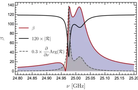
Figure 2.3.: Amplitude boost factor with a width of 50 MHz (red curve) produced by 20 dielectric discs of thickness 1 mm with a refractive index n = 5. Also shown are quantities correlated to the amplitude boost: the absolute reflectivity |R|

and the group delay

Arg( R ). Both quantities are scaled to be in the same order of magnitude as the boost factor. The reflectivity is calculated with a relatively high dielectric loss of tan δ = 5 · 10

to make it more pronounced. It can be seen that with such a configuration a quite top hat shaped power boost factor of ∼ 10

can be produced. Taken from [13].

The amplitude boost is defined as β ≡ |B| and the power boost as β

≡ |B|

respectively.

This means the axion signal output power is proportional to β

[13].

With the right distances between the discs a quasi continuous power boost over a range of frequency can be created. Therefore to control the frequency range for resonant signal enhancement the discs have to be variable in their position. Changing the distance between dielectric discs changes the width and height of the boost factor and also its position in the frequency space. A typical boost factor as it could be used in the final setup e.g. has a width of 50 MHz, cf. figure 2.3. With the possibility to shift the boost in a frequency range of approx. 10 GHz to 100 GHz MADMAX can scan a wide axion mass range between 40 µ eV to 400 µ eV.

2.1.4. Area Law

The boost factor is dependent on the frequency or equivalently the mass of the axion. Hence

to eventually cover the mass range of about 40 µ eV to 400 µ eV (the exact measurement

range is still a matter of ongoing discussion) a broadband response of the boost factor is

desired. The behavior of the boost factor over a frequency range can be predicted with the

so called ”Area Law”. The boost factor integrated over all possible frequencies for a given

configuration of disc distances is constant:

Z

0

β

dν = const . (2.7)

However this is only exact when considering the complete frequency range. If the majority of the boost is concentrated in the top hat it is a good approximation to only consider the limited frequency range covered by it. A realistic boost factor with a width of 50 MHz can be seen in figure 2.3. With the configuration of 80 discs used in this example an amplitude boost of ≈ 120 can be reached. According to the area law a half as wide boost could be approx. twice as large. Furthermore the boost factor can also be predicted for different setup configurations because the boost scales roughly linearly with the number of dielectric discs N in the system [12]. This is also a useful approximation since the exact number of discs for the final setup is not a fixed quantity yet.

2.2. Experimental R&D Efforts

After the introduction to the most important theoretical foundations of MADMAX we will now focus on the experimental setup properties. The most important setup properties will be named as well as the resulting experimental challenges and open questions which arise.

2.2.1. Receiver System

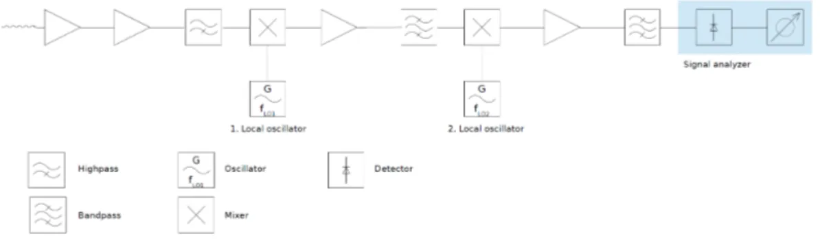
The receiver system for frequencies below 30 GHz is probably one of the most mature components of the setup. The microwave detection is based on preamplification using low noise HEMT (high electron mobility transistor) amplifiers followed by a heterodyne mixing of the pre-amplified signal. Figure 2.4 shows a scheme of this signal processing method.

First the signal is amplified by a low noise pre-amplifier stage. Afterwards it is pre-filtered by a highpass. The filtering is necessary to only process the frequency range of interest and exclude noise. After that the signal is mixed with a carrier frequency and therefore shifted to an intermediate frequency. The key feature of the mixing is that the signals are mixed in a non linear way [22]. Suppose that the original signal has a from sin(2πν

t) where ν

is its frequency and the carrier frequency has a similar form sin(2πν

t) with frequency ν

. The product of these two signals is then

sin(2πν

t) sin(2πν

t) = 1

2 cos(2π(ν

− ν

)t) − 1

2 cos(2π(ν

+ ν

)t) . (2.8)

The filtering after the mixing has then the purpose to filter out one of the obtained mixing

terms. Here the difference term of the two frequencies is kept. The shifted frequency in

this example then has the new frequency ν

= ν

− ν

. This mixing, amplification and

filtering scheme is applied until the resulting shifted, filtered and amplified signal can then

be detected by digital 16 bit samplers. These samplers also perform a real time fast Fourier

transform and store the signal data [9].

Figure 2.4.: The heterodyne mixing scheme. Shown are the amplifier, filtering and mixing stages. Taken from [9].

2.2.2. Proof of Principle Booster

A proof of principle booster to test the properties of a booster has already been built and test measurements have been performed. The booster itself consists of a mirror with a set of discs with a high material which is ideally positioned inside a waveguide. The first setup consisted of five sapphire discs ( ≈ 10) with 20 cm radius. The aim is to measure the group delay and reflectivity of the proof of principle booster. These quantities are correlated with the boost factor and if simulated group delay and reflectivity behaviors can be accurately reproduced with such a booster it proves that also a boost factor can be achieved with the needed accuracy. In figure 2.5 it can be seen that with five discs which are positioned by precision motors the necessary group delay behavior calculated with 1D simulation programs could be sufficiently well reproduced with the proof of principle setup. These tests indicate that also a larger booster could be controlled sufficiently well and the requirements for the final setup could be reached. Based on these encouraging measurements a larger 20 disc proof of principle setup has been designed which features up to 20 dielectric discs with 20 cm radius. The discs therefore have the same specification as in the 5 disc proof of principle setup. The new 20 disc proof of principle setup consists of a metal mount to which 10 rails have been attached to. Each of these rails carries two sledges which each have a mount to install a sapphire disc on this sledge. The sledges with the discs on top can then be moved with precision motors along these rails. The movement of the discs is similar as in the 5 disc setup but additionally the discs now also can be tilted in a controlled way and therefore the alignment of the discs can be further improved.

Vice versa the effects of tilts on reflectivity and group delay can be investigated. With

this larger setup also group delay results from simulations like in the 5 disc setup should

be reproduced and extrapolation to more discs can be tested. Also useful information on

controlling more complex setups are gained. The reproduceability of disc positions, the

efficiency of positioning algorithms for the discs or the reflection behavior of the total setup

can be tested. These and various other R&D efforts can be performed with the 20 disc

proof of principle setup. They yield experiences which will help to plan and understand the

full scale setup [23] [24].

Figure 2.5.: Transmissivity, reflectivity and group delay measurements with the five disc proof of principle setup. The disc positions were adjusted to meet the 1D simulation expectation and the agreement with the expectation is sufficient.

Left: measurement with 5 manually adjusted discs. Right: measurements of a 3 disc setup with disc spacings iteratively adjusted by an algorithm. Taken from [9].

2.2.3. Full Scale Booster Plans

While the proof of principle setup can be used to learn about important physical properties and resulting challenges for the booster, the full scale setup finally shall boost the microwave signal to a power sufficient to detect the axion in the proposed mass range of approx. 40 µ eV to 400 µeV.

State of the art radiometers in this frequency range can detect signals of ∼ 10

W within

one week of measurement time. The axion induced emission by a perfect mirror of 1 m

surface area inside a 10 T magnetic field however is only of the order of 10

W. We have

seen that with the help of dielectric discs of the same size as the mirror we can arrange a

booster setup to enhance the emitted signal. Discs and mirror much larger than 1 m

are

not feasible for current magnet designs which can create the required very large magnetic

fields. A bore to fit larger discs inside is technically difficult while maintaining a large

10 T magnetic field [12]. Neglecting any losses the required boost to create a detectable

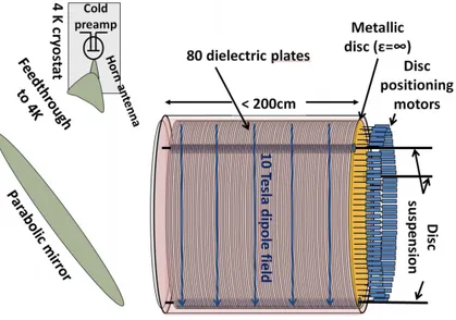
signal is ∼ 10

. This can be achieved by using 80 LaAlO

(lanthanum aluminate) plates

with a dielectric constant of = 24. With such a configuration a sufficiently high power

boost with a width of approx. 50 MHz can be created. A conceptual sketch of this setup

is shown in figure 2.6 [9]. However this is just a first concept for the final setup. Details

like e.g. the exact number of discs is still a matter of ongoing research. Also for example

the final magnet design is not fixed yet and various systematics of the booster have to be

understood. Loss mechanisms for example could play an important role to determine the

optimum number of discs.

Figure 2.6.: Conceptual drawing of the final MADMAX setup described in section 2.2.3.

Taken from [24].

2.3. Experimental Challenges and Open Questions

It is important to study the feasibility of building a full scale booster setup which can pro- duce the required boost factor. With proof of principle setups introduced in section 2.2.2 R&D efforts can be conducted. These setups allow to gather information how the full scale setup should be designed and what are the challenges for the projected measurement.

Another approach which simultaneously can be made are analytical considerations about the measurements with the full scale booster. One of these considerations is the total re- quired measurement time to be sensitive to the QCD axion in the projected mass range.

Several other topics are also connected to the measurement time i.e. they influence the sensitivity and therefore the required measurement time.

The motivation of this thesis is to investigate some of these issues and quantize them.

Noise Considerations

When scanning for signals, besides being able to detect a potential signal at all, noise in the receiver system is a limiting factor. The noise can be reduced by using low noise amplifiers and cooling devices, but still random noise fluctuations can mimic signals. The axion signal has an expected linewidth of 10

ν, where ν is the frequency at which the signal appears.

Noise fluctuations and signal look similar and therefore false signals have to be identified

and excluded. This results in a two stage measurement strategy: a broadband scan to cover

a range of axion masses and a rescan procedure where potential signals are re-measured with

a higher and therefore more narrow boost factor to prove or disprove the detection of a real

signal. Especially interesting here is if in fact the number of false positives obtained with

measurement of the already existing receiver system are as expected. An analysis of this

topic can be found in chapter 5. The statistical expectation of required re-measurements is utilized in chapter 7.

Loss Estimates

Losses are in general not desired. They lead to energy loss in the system and therefore reduce the effective power boost. Such losses can be caused by dielectric loss, diffraction, random tilts of the discs, unwanted reflections or other yet unforeseen effects. Simulations can be used to predict some losses e.g. the effect of tilts of the discs. A simulation approach therefore has been performed in chapter 3. Also a related measurement of the 20 disc proof of principle setup has been performed where the misalignment of the rails where the discs are mounted on was measured, cf. chapter 4. Still loss mechanisms have to be identified and quantified before effects on the booster can be reliably estimated. However, discussing loss in a generalized form can already be carried out to estimate the effect on the boost factor. This is described in chapter 6.

Readjustment Time and Measurement Strategy

Results from loss estimates and noise considerations are used to develop an optimum mea- surement strategy in terms of choosing feasible criteria for broadband and false positives re-measurements. The aim is to minimize the total measurement time necessary to de- tect the QCD axion with a certain significance limit. For some assumed parameters a set of optimum parameter choices are presented and a discussion of feasibility in reaching cer- tain optimum configurations is given. The discussion of this topic can be found in chapter 7.

We conclude in chapter 8 how the covered topics influence the development of the MAD-

MAX experiment and which challenges arise from the found results.

3. Simulation Approach with a 3D Raytracing Software

Some loss effects in the booster system can only be seen in a three dimensional environment.

Especially loss that is caused by radially asymmetric geometries like tilts of the discs can only be simulated in a three dimensional environment. In this chapter we discuss the use of a ray tracing software to simulate such issues. Ray tracing is one possible simulation method. We introduce the basic working principle of ray tracing and discuss why it should be a suitable method for simulating the MADMAX booster. The software tested for the simulation is called OpticStudio Zemax [25]. Simple basic setups have been tested to verify if one dimensional simulations can be reproduced and therefore if the program is suitable to model more complex setups and their potential loss mechanisms. Ideally a simulation of the full scale 80 disc setup should be carried out.

3.1. Ray Approximation

In ray tracing algorithms the ray approximation of electromagnetic radiation is used. Rays are normal to the local wavefront of the electromagnetic wave and point in the direction of the energy flow of the wave, i.e. the Poynting vector. Hence a ray models a part of a plane electromagnetic wave and its propagation direction is equivalent to the propagation direction of the wave. The ray model is especially simple in the case of homogeneous, isotropic media. In this case the rays are simply straight lines. When propagating through an optical system rays can interact at the surface between different media. Commonly they can refract, reflect or diffract which alters their direction of propagation but possibly also other properties such as the phase of the wave associated with the ray.

The rays have a set of physical properties. For the propagation the current position of

the rays and their direction of propagation have to be tracked. Since rays approximate a

wave front also information on the amplitude and phase are assigned to the rays. For some

propagation methods also polarization can be included. The energy a ray carries is defined

by its amplitude. A total wavefront is represented by many rays where each ray describes

a patch of this wavefront. Therefore the ray approximation can be best used when the

waves can be modeled as plain waves. Usually also for naive ray tracing approaches the

wavelength of the rays should be far greater than the size of the objects so that diffraction

can be neglected. In our MADMAX setup we deal with wavelengths on the millimeter to

few centimeter scale. The dimension of the discs in the final setup are supposed to be on

the order of approx one meter. Hence the ray approximation should be suitable for our

problem from this perspective.

The main reason we think of using a ray tracing software is that it does not explicitly solve the Maxwell equations. The computation effort therefore is expected to be substantially lower and hence the simulation faster or respectively can be more complex than e.g. in a finite element solver which numerically solves the Maxwell equations. For the basics of ray tracing and ray approximation also cf. [26].

3.2. OpticStudio Zemax: A Ray Tracing Software

In this section the parts of the ray tracing software OpticStudio Zemax which are neces- sary to perform a basic simulation of MADMAX are explained. Zemax Optic Studio is a commercial software designed to analyze, simulate and optimize optical systems with a ray tracing approach.

The used version of Zemax for the simulations in this chapter was OpticStudio 15 SP1.

3.2.1. Simulation Modes

Before the simulation approach is described the chosen simulation mode has to be fixed since the way the simulation components and the simulation itself work depends on this mode. Zemax can use two different simulation modes to simulate optical systems. These modes are called sequential mode and non sequential mode.

Sequential Mode:

The key property of the sequential mode is that it works with surfaces. The rays are traced from surface to surface starting from a source. The propagation is performed in the order these surfaces are listed in the program editor. So every ray is traced for a fixed sequence.

This mode is therefore preferred for systems that require optimization, tolerancing and a detailed image analysis. Such a system could be for example a series of different lenses.

In this mode rays cannot interact multiple times with the same surface, i.e. multiple reflections are not accounted for and resonant behavior cannot be simulated. Therefore this mode is not suitable for us.

Non-Sequential Mode:

The non-sequential mode is the complementary mode to the sequential one. Instead of defining surfaces, the non-sequential mode uses volumes in 3D space. The huge advantage when performing a simulation in comparison to the sequential mode is that in this mode the rays are traced in a physical manner instead of following a fixed propagation scheme.

Also rays do not only make a single interaction per object but they can be transmitted and

reflected multiple times. This means the simulation needs thresholds which define when the

simulation can be stopped. These thresholds are the maximum number of intersections per

ray, the maximum number of segments per ray and the relative energy threshold. When

rays interact with the objects child rays are formed, i.e. for example for a generic reflection

part of the ray gets transmitted and part of it is reflected. That means the original ray gets

split up into two rays. How many child rays can be formed per original ray depends on

the simulation settings this setting is called the maximum number of intersections. Zemax allows up to 4000 intersections which we have also chosen as the threshold for our simulation.

The total path of a ray consists of many segments. A segment is defined as the part of the ray between two interaction points, e.g. the path between the source and the first intersection with a surface defines the first segment. A limit also exists how many segments are allowed per original ray. In the example of a generic reflection the ray is split up into two child rays, these two rays then count as segment two and three. The maximum number allowed here is 2,000,000 segments per ray. We have chosen 5000 segments per ray as the simulation threshold.

The last threshold is the minimum relative energy threshold which defines at which energy relative to the starting energy of a ray the tracing will be stopped. We have chosen 10

as the relative energy threshold [27]. That these limits are sufficient for our simulation can be seen in section 3.4.1.

Another important setting that can be fixed at this point is the wavelength of all rays used in the simulation. For the tested simulation setups frequency sweeps have been performed for the frequency range from 10 GHz to 30 GHz. Each sweep consists of 500 individual ray tracing simulations where for each ray trace the frequency has been changed. The steps between the simulated frequencies is equidistant.

3.2.2. Simulation Components in Non-Sequential Mode

So far we discussed which operating mode of Zemax to use. To interpret the results of the simulation tests we will introduce the most important components of the simulation software needed to create a simulation environment. The following informations were extracted from [27].

Sources

Rays are inserted into the simulation by source objects. Sources are special objects in the simulation domain. They can be point-like or surfaces from which the rays are emitted.

The starting properties of the rays such as the power, wavelength and polarization are controlled here. For the simulation a rectangular source has been chosen. These source emits rays perpendicular to its surface and the starting position of each ray is randomized.

The total power of the source has been fixed to 1 W while this power is equally distributed across all started rays. The starting phase for all rays has been chosen to be 0. Note also that the source objects have no impact on the simulation, rays do not interact with sources.

Objects

The main content of the simulation is made up by objects. Objects are geometrical forms like cylinders, cones or cuboids.

The objects can be freely placed and rotated in 3D space and the size and material compo-

sition can be controlled with the editor tool. The main property of a material is the index

of refraction as it defines the transmitted and reflected amount of radiation. For incident

radiation on a surface the reflection and transmission coefficients can be calculated with the Fresnel formulas, cf. [28].

Since the refractive index is in general not independent of the wavelength Zemax can use different formulas to interpolate the refractive index for different wavelengths given refer- ence points. Additionally to the refractive index also absorptive properties and other for our simulation non relevant properties can be specified.

For the material of the discs we want to implement in the simulation we have to define our own material because the materials supplied by Zemax itself are only defined for wave- lengths approx. in the visible spectrum and not for microwaves as we need it. For simplicity we set the refractive index of our material constant over the specified frequency range. This is consistent with 1D calculations conducted of the booster.

We have specified the material which we used for the dielectric discs equivalent to sapphire which has been used for the proof of principle setups. This material therefore has a refrac- tive index of n = √

= √

9.2. For the mirror no material has to be specified because Zemax already supplies a perfect mirror material.

Detector Objects

The last piece needed for a complete simulation are detector objects. Detector objects are similar to source objects as they do not interact with rays and do not influence the simulation. They allow to store the information of the rays. The information carried by the rays is the intensity and phase. The complex electric field is calculated from it by Zemax.

The detector objects are divided into pixels and return information on the rays pixel-wise.

The electric field amplitudes of all rays that hit one specific pixel are therefore summed up.

That means that at the evaluation time of the rays interference is possible. In the following simulations a detector with a single pixel will be used because the antenna in the actual setup also provides no spatial information on the incident waves. However, we therefore imply that all rays equally interact with each other. This can be assumed since the first 3D simulations shall be equivalent to 1D representations of the setups.

3.3. Simulation Approach

For the test simulation we conduct four different test cases. In this section we introduce these four test cases and also the theoretical properties which are necessary to analyze the test setups. These test cases are kept simple so that it is possible to compare the simulation results to theoretical expectations or 1D simulations. Theoretical expectations and 1D simulations should be reproduceable with Zemax. The 1D expectations are calculated using the program ”Qucs” [29] which performs calculations that are equivalent to the transfer matrix formalism, cf. section 2.1.3.

The quantities of interest are especially the phase and group delay of a reflected signal of the

setups and also the total intensity since loss mechanisms can have a significant impact on

the results [23]. The group delay is an important measure of a setup because this quantity

is correlated to the power boost factor in MADMAX.

3.3.1. Simulated Test Cases

Four test setups are presented here: a perfect mirror and a source, one dielectric disc and a source and a dielectric disc and a perfect mirror combined with a source. The latter is split up into two setups, one with disc and mirror in contact and one with an air gap between disc and mirror. A sketch of these setups can be seen in figure 3.1.

General Simulation Properties:

Some of the simulation settings are identical for all four simulations. All rays are launched in parallel in z-direction and from a surface smaller than the geometry of the objects so that no ray misses any setup component. The object surfaces are also perfectly parallel to each other in the x-y-plane such that rays cannot scatter out of the system due to reflections.

This ensures that the simulations are equivalent to a 1D description which is necessary since we want to compare the results in Zemax to 1D calculations. As mentioned previously both the calculations and simulations have been performed for frequencies between 10 GHz to 30 GHz with frequency steps of 40 MHz in the case of the Zemax simulations.

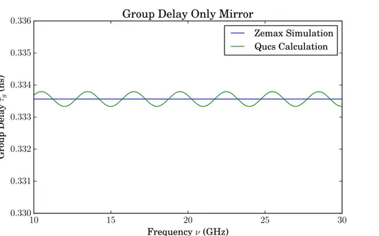
1. One single perfect mirror:

The simplest simulation case is shining microwaves onto a mirror. A perfect mirror just reflects 100% of the incident radiation. The distance between the mirror and the source and detector is set to 50 mm. Zemax supports an idealized mirror material which should represent a perfect mirror. All rays get reflected but the mirror material implicitly is assumed to be aluminum which causes an absorption loss. Therefore to make the mirror ideal an ideal reflection coating was used. This coating reflects 100%

of the incident radiation equaling a perfect mirror. An ideal reflection coating can be defined by specifying the reflection and transmission coefficients to be 100% and 0%

for all wavelengths respectively [27].

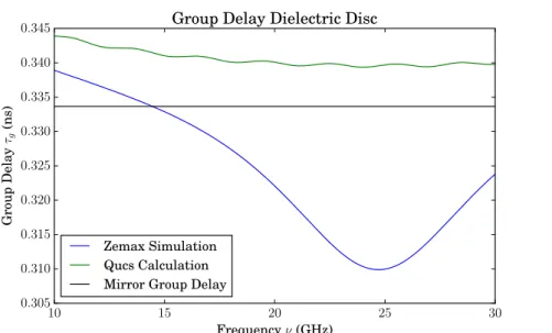
2. One dielectric disc:

This setup consists only of a dielectric disc with a permittivity of = 9.2 which is similar to the sapphire discs used in the current 5 and 20 disc MADMAX proof of principle setups. The distance between detector and disc again is 50 mm. The thickness of the disc is 1 mm. This disc thickness is equivalent to the sapphire discs used in measurements.

3. Dielectric disc on top of a perfect mirror with no gap in between:

This setup combines a perfect mirror and a sapphire disc. The properties of mirror

and disc are as described in setup 1 and 2. The distance from source and detector to

the disc is 50 mm and the mirror follows directly after the disc with no additional air

gap.

Figure 3.1.: The four test simulation setups. The grey bars depict perfect mirrors and the blue bars dielectric sapphire discs with = 9.2. The solid black lines show the position of the source and detector. Not to scale.

4. Dielectric disc and a perfect mirror with a gap in between:

Setup 4 is obtained by separating the disc and mirror in setup 3 by an air gap which is 8 mm wide. A distance of 8 mm was chosen because it is a common benchmark width used for example in the proof of principle setups and 1D calculations corresponding to a booster for ν ≈ 18.7 GHz. The distance from the source and detector to the disc is 50 mm and the properties of the disc and mirror are the same as described in setup 1 and 2 previously.

3.3.2. Theoretical Simulation Expectations

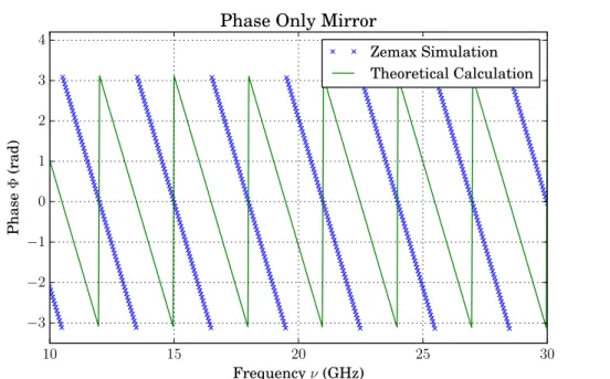
In this section important theoretical expectations are introduced. Primarily we want to check if the reflective properties especially the group delays of the test setups are as ex- pected. These properties are correlated to the boost factor, cf. [9], and therefore it is convenient to calculate them since these quantities also can be measured with actual proof of principle setups. Therefore we calculate the phase of the rays at the detector which allows us to derive the group delay from it. Additionally the intensity measured at the detector is recorded. This allows to detect energy loss which is relevant since energy loss influences the group delay and therefore the boost factor.

Phase

The phase is the basic information we can extract from the reflection. It is the argument of the reflected field amplitude. In some simple setup cases like case 1 we can analytically calculate the expected phase over the frequency. The phase evolves due to the traveled path length in the system and possible phase shifts due to reflections. Therefore the total phase of a detected ray is expected to be

Φ

= 2π

c · νnx + N · π . (3.1)

Here ν is the frequency, n the index of refraction of the medium, x the total physical path

length for the rays and N the number of reflections that cause a phase shift of π.

The phase in Zemax is represented as an angle between ( − π, +π). The theoretical phase therefore has to be shifted to this interval since from the formula above the theoretical calculated phase Φ

would lie between (0, 2π) and respectively multiples of this interval.

We call the phase obtained in Zemax Φ and define the shifted phase Φ

which should fulfill

Φ

≡ Φ . (3.2)

Therefore we apply the following shift to the phase Φ

which is in the interval between (0, 2π) (and multiples of it):

(0, 2π) −−→

(π, 3π) −−−−−−→

(π, 2π) and (0, π) −−→

(0, π) and ( − π, 0) (3.3) With this shift we have mapped the original phase interval (0, 2π) to the interval ( − π, π) where (0, π) is unchanged and (π, 2π) is now equivalent to the interval of ( − π, 0).

Written as one equation the shifted phase Φ

is obtained by

Φ

= ((Φ

+ π) mod 2π) − π . (3.4)

The obtained phase from the simulation and the theoretically calculated phase are equiva- lent.

Group Delay

Qualitatively the group delay can be understood as a measure how long a signal of a certain frequency stays in the system. The group delay τ

is defined as

τ

= − dΦ

dω (3.5)

where it represents the change rate of the total phase shift Φ in dependence of the angular frequency ω. Therefore the phase of the reflected signal is a measure for the phase response of the tested system.

Coherent and Incoherent Intensity

The intensity measured at the detector can be calculated in two different ways. One method is to sum over the intensities P

of all rays and the other method is to add up the elec- trical field components E

exp(iφ

) of all rays. We call the obtained intensities from the first method the incoherent intensity P

and the intensity from the second method the coherent intensity P

.

P

= X

i

P

(3.6)

P

=



 X

j

E

e





2

(3.7)

The incoherent intensity is a special case of the coherent intensity when the averaged phase relation between the rays is random and therefore the interference terms E

E

exp(i(φ

+ φ

)) cancel out. The launched rays in our case are coherent which means that the correct way to calculate the intensity is calculating the coherent intensity. However, using incoherent intensity we can directly see if in the setup some of the rays lose energy in any way. If no energy is lost the incoherent intensity equals the input power for a system with total reflectivity of one as it should be the case for test setups 1, 3 and 4.

When calculating the coherent intensity also phase information is included. Hence this intensity allows us to observe if any interference effects appear. As we start the simulations with coherent rays we can expect that interference effects will occur. However, it is ana- lytically difficult to predict how the different ray generations interfere with each other and which value of the coherent intensity we have to expect for a certain frequency.

Outgoing Electric Field Amplitude in Test Setup 3:

The complexity of setup 3 is high enough that multiple generations of reflections occur and it is simple enough that we can still calculate the total reflected field amplitude of this system. It is therefore possible to theoretically predict the coherent intensity for a specific wavelength in this case which we can then compare to the obtained results from the simulation. The ingoing electromagnetic wave is considered to have an amplitude A

≡ 1 and if this amplitude is split up into multiple rays they are supposed to be coherent. At the dielectric disc surface the incoming wave is split up in a reflected part A

and a transmitted part A

where the transmission and reflection coefficients are given by the Fresnel formulas, cf. [28]. The continuity condition at the surface demands that A

= A

+ A

. The amplitudes then evaluate to

A

= r · A

(3.8a)

A

= A

+ A

(3.8b)

= (1 + r) · A

(3.8c)

where r is the amplitude reflectivity between air and the dielectric disc. The transmission coefficient from air to disc is t

= 1 + r which has implicitly already been substituted here.

The second boundary is the mirror. Here everything gets reflected and only a phase shift of π is introduced which is equivalent to a reflection coefficient of

r

= − 1 . (3.9)

The reflected wave finally hits the surface between disc and air and part of the wave is

again reflected and the other part transmitted. The reflection and transmission coefficients

are