in two-band systems and

(1)

(2)

Phillipp Reck

Quantum echoes and revivals in two-band systems and Bose-Einstein condensates

(3)

Herausgegeben vom Präsidium des Alumnivereins der Physikalischen Fakultät:

Klaus Richter, Andreas Schäfer, Werner Wegscheider

Dissertationsreihe der Fakultät für Physik der Universität Regensburg, Band 52

Quantum echoes and revivals in two-band systems and Bose-Einstein condensates Dissertation zur Erlangung des Doktorgrades der Naturwissenschaften (Dr. rer. nat.) der Fakultät für Physik der Universität Regensburg

vorgelegt von Phillipp Reck aus Erlangen im Jahr 2017

Die Arbeit wurde von Prof. Dr. Klaus Richter angeleitet.

Das Promotionsgesuch wurde am 30.10.2017 eingereicht.

Prüfungsausschuss: Vorsitzender: Prof. Dr. Franz Gießibl 1. Gutachter: Prof. Dr. Klaus Richter 2. Gutachter: Prof. Dr. John Schliemann weiterer Prüfer: Prof. Dr. Tilo Wettig

(4)

Phillipp Reck

Quantum echoes and revivals

in two-band systems and

Bose-Einstein condensates

(5)

Bibliografische Informationen der Deutschen Bibliothek.

Die Deutsche Bibliothek verzeichnet diese Publikation

in der Deutschen Nationalbibliografie. Detailierte bibliografische Daten sind im Internet über http://dnb.ddb.de abrufbar.

1. Auflage 2018

Umschlagentwurf: Franz Stadler, Designcooperative Nittenau eG Layout: Phillipp Reck

Druck: Docupoint, Magdeburg ISBN: 978-3-86845-154-2

Weitere Informationen zum Verlagsprogramm erhalten Sie unter:

www.univerlag-regensburg.de

(6)

Chapter 1 Introduction – a tiny story of time, including demons

Philosophically, the flow of time has probably always been a mystery for mankind.

Although is seems not to be as fundamental as the question about the sense of life, which practically everyone wondered about for a longer or shorter time before turning one’s attention to more pragmatic issues, many great thinkers dedicated themselves to the affairs of time.

Already in ancient Greece in the pro-Socratic philosophy [1], there were two words for time (which of course had their godly personification): Chronos and Kairos. While the first stands for the steady flow of time which can be measured quantitatively, the other describes the time felt individually and the time for the right moment.

Also in the literature, time is a reoccurring subject, most of all in modern science fiction. The possibility of time travels is played out in uncountable stories with all of its implications and paradoxes like meeting oneself and influencing the past. The consequences are visualized by the trousers of time: one starts in one leg (present), going up to the waistband (past) and changing the conditions there such that one goes done the other leg leading to a different present. Related to this metaphor is the multiverse theory that “everything happens somewhere”, where somewhere might mean a hypothetical parallel universe.

From a physical point of view, the flow of time in only one direction (future) has been coined as the arrow of time by Arthur Eddington [2]. With the formulation of the laws of thermodynamic in the 19th century at the latest, the arrow of time was considered in modern physics, e.g. by Boltzmann [3] and Loschmidt [4]. The important corresponding thermodynamic theorem is the second, which says that the entropy of a closed system increases over time. Although the arrow of time poses some fundamental questions (“Why is there an arrow of time; that is, why is the future so much different from the past?” [5]), the entropy seems to be the classical observable by which one can tell the chronological order. As an easy example, think of two photos of a flower vase: in one picture, it is intact, in the other one, hundreds of shards are visible. Which photo has been taken before the other one? In other words, which picture shows the higher ordering of the involved particles?

There have been many gedankenexperiments trying to violate the second law of thermodynamics often involving some kinds of demons [6]. A famous example is

(9)

1.Introduction – a tiny story of time, including demons

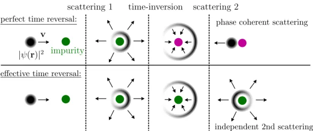
the Maxwell demon, which sits on a gate between two closed boxes filled with air of the same temperature allows the passage of particles from left to right only if their kinetic energy is below average and from right to left if above average. Another less famous demon, which is more closely related to our work, is the Loschmidt demon. Consider two adjacent boxes, one filled with air, the other one with vacuum.

Upon connecting the two boxes, the air particles will flow out of the filled box and distribute uniformly in the enlarged volume. This state has a higher entropy, since there are again more micro states for the uniform distribution in the larger box than in the smaller one. Now, the demon comes into play. By perfectly inverting the motion (v→ −v) of any gas particle in the system (and considering perfect elastic collisions between particles), every particle would propagate back exactly the time- reversed way, bouncing off of the same particle as it did before the inversion and finally going back to the initial box. Although the boxes are still connected, every particle is now again in the initial volume, which means that the entropy recovers its initial value, thus violating the second law. The problem of the realization of this demon is obviously the difficulty of reversing the motion of all the particles individually. The possibility of an experimental realization is worsened by the fact that the velocity-inversion has to be strictly perfect due to the chaotic behavior of the many-body systems – even if only one particle is not perfectly reverted, but moves let’s say in a slightly different direction, all of its prior collisions will not take place the way they did before. Therefore, all the particles it collided with are not going back to their initial position. But equally in the next step, all those particle will not collide with the particles they did before the process. This exponentially growing deviation from perfect time-inversion will lead in the end not to the recovery of the particles in the smaller volume, but again to a uniform distribution in the larger volume.

Despite the non-realizability of the initial Loschmidt demon, time-inversion protocols have been invented for all kinds of systems in the 20th century. Maybe the first and certainly one with the highest applicability is the spin echo developed by Hahn in the 1950’s [7]. The echo makes use of the nuclear magnetic resonance (NMR) discovered by Bloch [8, 9] and Purcell [10], for which they were awarded the Nobel prize for physics in 1952. The idea behind the NMR is that magnetic moments, here the nuclear spins, rotate around a static, perpendicular magnetic field of strengthB with the Larmor frequency ω_L =γB, where γ is the gyromagnetic ratio. However, due to inelastic interaction with its environment, a nuclear spin will align along the direction of the magnetic field on the time scale T₁ of the order of some 100 ms to a few seconds [11]. An additional radio frequency pulse close to resonance with the Larmor frequency rotates the direction of the spin an arbitrary amount away from its aligned position, e.g. perpendicular to the magnetic field (π/2-pulse).

In general, not a single nuclear spin is manipulated but a macroscopic ensemble, e.g. all the nuclei of the hydrogen atoms in water molecules. There, the Larmor frequency of the nuclear spins is given by ω_L ' 42.6 MHz×B[T]. After a π/2- pulse, all spins are perpendicular to the static magnetic field and therefore rotate (in phase). Since rotating magnetic moments emit electromagnetic radiation, this rotation can be measured. However, due to slightly different environments and thus different local magnetic fields of close magnetic moments, every spin rotates with

(10)

a slightly different Larmor frequency. The more the rotation of the spins is out of phase, the more the emitted radiation interferes destructively until no signal is measured. The related decay time is called T₂^∗ and is in general much smaller than T₁.

The spin echo, also called Hahn echo, effectively time-inverts the dephasing process related to T₂^∗. Thereto, an additional π-pulse is needed. The spins, which are in a plane perpendicular to the static field, are therefore rotated by 180^◦, so that they are still in the same plane, but inverted, meaning that the faster rotating spins find themselves ”behind“ the slower ones, catching up over time, and the ensemble rephases again, which leads to a measurable echo.

This ”catching up“ process works of course only as long faster rotating spins stay faster, i.e. as long as the environment does not change. In an experiment, this environmental change will happen and its effect can be measured in an exponential decay with the time scale denoted T₂, which cannot be reverted by the spin echo.

For technical application of the spin echo, like non-invasive imaging of biolog- ical tissue, all kinds of modifications and extensions are applied, such as making the external magnetic field (and therefore ω_L) position dependent, to get spatially resolved pictures [12, 13], for which Lauterbur and Mansfield got the Nobel prize in medicine in 2003. The technical enhancements are such that although early NMR needed up to an hour for making a single picture, it is nowadays even possible to make real-time videos, i.e. more than 24 pictures per second, that can be watched immediately [14, 15].

Note that in this setup, there are quite some differences to an (effective) time- inversion, e.g. the precession direction of the spins does not change as it would for a time-inversion, but instead the trick is to bring the fast spins behind the slow ones. Nevertheless, since the spins rephase and therefore the emitted signal can be measured as an echo, it seems as if the time has been inverted. Therefore, the spin echo as an effective time-inversion protocol can be seen as the first time mirror protocol for a macroscopic, classical ensemble of individual quantum system, however for a discrete Hilbert space (spin 1/2).

Our goal is a time mirror protocol for the wave function of a quantum system, e.g. an electron in a solid, thus for a continuous Hilbert space. Therefore, let us consider what is known of time-reversal mirrors for classical systems with continuous degrees of freedom, i.e. classical waves, and whether the techniques are transferable to quantum wave functions.

Since the late 20th century, time-reversal mirrors have been of practical importance in many fields like medicine, telecommunication, material analysis, and gener- ally in wave control [16–19]. They have been realized with all kind of classical waves like sound [20,21], elastic [16], electromagnetic [22] and recently water waves [23,24].

The basic concept is the following. An initially localized wave propagates through some locally confined random medium in which it is scattered. Outside of the scattering region, an array of receiver-emitter antennas measures and records the incident wave amplitude as function of time at many positions. After some time the signal is rebroadcast from each position, however in time-inverted manner, i.e. which came in last is emitted first. Thus, similar to the case of the Loschmidt demon, any scattering process takes place the same way (but backwards), such that the wave

(11)

is finally refocused to its initial position, as long as the random medium does not change over time [25–27].

The great advantage compared to the chaotic behavior of the gas particles discussed above, which mainly scattered among each other, is that the scattering process for the wave is not chaotic. The reason for this can be heuristically motivated by the following argument: changing the initial condition of a discrete particle (e.g.

a ball) going through a random scattering might lead to missing the first obstacle, for instance, which will lead to a completely different trajectory. An extended wave (or at least parts of it) on the other hand, will always hit the obstacle, such that a slight change of initial conditions only leads to a slight change of the trajectory.

Therefore, even if the rebroadcast of the individual emitters is not perfect, an echo of the initial wave is achieved. For visible light, this time-inversion mirror is difficult to implement due to missing controllable antennas [19]. Nevertheless, time-reversed waves can also be generated for monochromatic light, using three- or four-wave mixing [28, 29].

The problem of the measuring-rebroadcasting protocol for a quantum wave function is apparent: a measurement at one position will heavily influence the outcome of all other measurements due to the projection axiom in quantum mechanics. Thus, for the quantum time mirror in a continuous Hilbert space, other methods have to be applied. An alternative to control the wave via the spatial boundaries is a ma- nipulation via time boundaries [30–36]. Similar protocols were considered, using time- and space-modulated one-dimensional photonic [37–39] and magnonic crys- tals [40, 41]. For a specific, one-dimensional propagation, time-reversal protocols have been proposed [42, 43] and realized in a kicked rotor model of atomic matter waves [44], but only in a narrow momentum range.

The new development of the so-called instantaneous time mirror (ITM) [45] has been the initiator of the idea for the proposed quantum time mirror (QTM) protocol in this thesis. In their work, Bacot et al. show the effective time-inversion of the motion of water waves by applying a short disruption to the system, after which each wave peak splits and parts of it propagate back in the opposite direction to the initial position. The sudden modification they use is a short change of the gravitational potential by accelerating the bottom of the box filled with water, which generates effective source terms in the wave equation, called ”Cauchy sources“, which define new initial conditions that lead to a partial reversion of the waves propagation, in agreement with the Huygens-Fresnel principle. Although the time-inversion is not perfect (actually, the ”reflected“ wave is proportional to the time-derivative ∂φ/∂t instead ofφ), distinct echoes are not only seen for radially spreading waves generated by a point source, but also for more complicated initial wave structures, like a smiley of the Eiffel tower.

The important feature of the ITM is the fact that no knowledge of the wave structure and thus no measurement is needed at the time of the homogeneous pulse.

Therefore, this basic scheme is in principle transferable to quantum systems. How- ever, a direct transfer is not possible because of the very fact that the differential equations governing the time-evolution deviate in the case of water waves and quantum systems. Nevertheless, we want to generate similarly an echo of quantum wave packets by applying a short time-dependent perturbation (e.g. a potential V(t)),

(12)

which is homogeneous in space. Since no measurement is involved, the system will continue to propagate according to the Schr¨odinger equation, without being pro- jected to the respective eigenstates of the measured observable. The important point is to make sure that the velocity of parts of the wave packet change sign, such that they move back to the initial position.

The thesis is organized as follows.

In chapter 2, the basic principles and tools used in the thesis are presented.

First, we give a short overview of graphene and derive its low energy band structure, since it is the physical system mainly considered in the thesis. As we are interested in the propagation dynamics, the unusual constant magnitude of the velocity of electrons in graphene is stressed. Moreover, the main numerical tool used to propagate wave packets is briefly presented, which is the time-dependent quantum transport (TQT) library developed by Viktor Krueckl [46].

In chapter 3, the first proposed quantum time mirror setup is investigated in graphene, as representative of any two-band system that is effectively described by the massless Dirac equation. The time-dependent potential briefly opens a gap such that the initial eigenstates undergo some kind of Rabi-oscillation and partly end up in the other band which has an opposite propagation direction. Therefore, one could speak of the ”population inversion quantum time mirror“. The mechanism is verified both analytically and numerically and the effects of shape changing of the wave packet, the behavior for long pulses, as well as its mode of action for more complex wave structures is studied. The chapter ends with a discussion about problems and possibilities for an experimental realizability of this Dirac QTM, as well as an overlook of the areas of research which might profit from the effective time-inversion.

Inchapter 4, the Dirac QTM discussed in the previous chapter is revisited and investigated for static perturbations to the Dirac Hamiltonian in regard of the question of whether the effective time-inversion is destroyed or unaffected. Therefore, the QTM with specific kinds of perturbations – disorder, electric and magnetic fields – is investigated both, analytically and numerically. Moreover, in a general section, any kind of static perturbation is discussed to be able to anticipate its qualitative action on the QTM. An outlook is given in which the possibility of using time-dependent electromagnetic fields as alternative way to induce the needed transition from one band to the other, is discussed.

In chapter 5, the population inversion QTM mechanism is generalized for any effective two-band system, where on the one hand requirements are derived for the effective time-inversion to happen at all, and on the other hand, the quantitative echo strengths are derived if these requirements are fulfilled. The general, analytical findings are numerically verified in three example band structures, linear bands with different slopes, the gapped Dirac equation, i.e. hyperbolic bands, and parabolic bands with different curvatures.

Inchapter 6, a different echo mechanism is studied for the nonlinear Schr¨odinger equation, which describes for instance the propagation of the ground state of a Bose- Einstein condensate (BEC). Here, the nonlinear part is used to effectively accelerate the wave function so that parts of it reverse their direction of motion. Moreover, with the same principle the broadening of the wave function, related to Heisenberg’s

(13)

uncertainty principle, can be inverted and the wave function refocuses again. Instead of a time mirror, we denote this refocusing setup by a ”time lens“ due to its optical analogy. Using the lens pulse over and over again, the broadening of the wave function can be prevented over long times and even approximate solitonic solutions, i.e. waves that don’t change their shape, can be achieved.

In chapter 7, the zitterbewegung of electrons in graphene is discussed. After an extensive introduction about the well-known decay of zitterbewegung for wave packets in the static case, we explore its behavior in a driving potential with the hope of getting long-time surviving modes. Although this chapter seems to be completely independent of the rest of the work, the relation to the population inversion QTM becomes visible when a mass pulse is used to invert the afore-mentioned decay of the zitterbewegung, leading to an echo, similar to the Hahn-echo. In a disordered setup, we show exemplarily that the echo strength, i.e. the ratio between revived and initial amplitude, behaves similarly to the echo fidelity, which means that it decays exponentially with the elastic scattering time, but unlike the echo fidelity, the zitterbewegung is in principle a measurable quantity. Due to its similarity to the Hahn echo, one could now think of using the well-known techniques, e.g. to get an spatial resolution of the elastic scattering time, and thus disorder strength, in a sample.

Inchapter 8, the findings of this thesis are summarized and an outlook is given on possible future research directions of the QTM.

(14)

Chapter 2 Basic concepts

2.1 Graphene

2.1.1 Low energy Hamiltonian

The first theoretical appearance of graphene was already 65 years ago, when P. Wal- lace [47] used a two-dimensional, hexagonal lattice of carbon atoms (graphene) as a first approach to graphite, which consists of many such layers that are stacked one above the other and coupled by van der Waals forces. In the following decades, graphene was used as a model system to understand more complicated carbon al- lotropes, e.g. carbon nanotubes, and it was theoretically investigated due to the surprising analogy to relativistic quantum mechanics for small energies [48–52], although it was predicted that as a strictly two-dimensional structure, it is thermo- dynamically unstable [53, 54]. Therefore, it was very surprising when in 2004, K.

Novoselov and A. Geim [55] were able to produce single layers of graphite: graphene.

The unexpected existence of free-standing graphene can be explained by the stabi- lizing effect of slight crumbling [56]. The discovery was honored 2010 by the Nobel prize for physics and lead to an enormous increase of research interests in the field of graphene, not only because of its high charge carrier mobility and mechanical stability due to the σ-bonding of neighboring atoms.

Although the original method, the mechanical exfoliation from highly ordered pyrolytic graphite, produces high quality graphene flakes, it is not suitable for mass production, as only a few of the exfoliated flakes are single layers which have to be picked out manually. Therefore, other methods have to be deployed like the epitax- ial growth on SiC [57, 58] by making use of the effect that by rising temperature, the silicon atoms vaporize first, leaving behind only the carbon atoms which then form a graphene sheet on the surface of the SiC crystal. Another method is the chemical exfoliation, which again obtains graphene out of highly ordered graphite, but instead of pealing off individual layers mechanically, the van der Waals interac- tions are broken by ultrasonication. The resultant flakes are stabilized by a chemical detergent and can be put on a substrate of choice [59, 60]. Nowadays most promis- ing for applications as electrical devices (e.g. transistors) is ultraclean graphene, i.e.

graphene encapsulated in hexagonal Boron-Nitride (hBN), with has among others the advantaged that it is flat, it is relatively free of charge puddles and dangling bonds and it has a very similar lattice constant to graphite, such that almost no

(15)

2.Basic concepts

(a) (b)

Figure 2.1: (a) The graphene honeycomb lattice is shown with the lattice vectors a₁ =a(1,0) anda₂ =a(¹₂,

√3

2 ) and the vectors between the nearest C atom neighbors R1 =aCC(0,1), R2 =aCC

−

√ 3 2 ,−¹₂

andR3 =aCC

^√

3 2 ,−¹₂

. The surface that is marked blue is the unit cell. There are two nonequivalent C atoms in the unit cell called A(blue) and B(orange). Panel (b) illustrates the Brillouin zone in reciprocal space with the reciprocal lattice vectorsg₁ andg₂. The corners of the Brillouin zones are theK-points which are connected to each other by reciprocal lattice vectors and the K⁰-points.

strain is induced [61]. The encapsulation protects the graphene from environmental influences and keeps it clean such that mean free paths of the order of 28µm [62]

and more are possible.

In this subsection, we want to derive the low energy Hamiltonian of graphene in the tight-binding approach. There are numerous publications showing this deriva- tion and we will follow notation-wise and conceptually Sasaki and Saito [63].

As already mentioned, graphene is a two-dimensional lattice of carbon atoms which are arranged in a hexagonal structure as shown in Fig. 2.1(a). The primitive translations are given by the two lattice vectors a₁ = a(1,0) and a₂ = a(¹₂,

√ 3 2 ), where a = √

3a_CC ≈ 2.46˚A with a_CC ≈ 1.42˚A being the bond length between the two neighboring carbon atoms. An important fact is that there are two carbon atoms (often called A and B sites) in the unit cell, which leads to several interesting consequences for the electronic structure as discussed below.

The Brillouin zone is a hexagon which is rotated with respect to the real space hexagon by 90^◦, see Fig. 2.1(b). The reciprocal lattice vectors are g₁ = ^2π_a

1,−^√¹₃ and g₂ = ^2π_a

0,^√²₃

. The adjacent corners of the Brillouin zone (the K-points) are not equivalent as they are not separated by the reciprocal lattice vector. Thus there are two triplets of equivalent K-points: K₁ = ^2π_a ²₃,0

, K₂ = ^2π_a

−¹₃,^√¹₃ and K₃ = ^2π_a

−¹₃,−^√¹

3

, connected to each other by reciprocal lattice vectors and K⁰₁ = −^2π_a ²₃,0

, K⁰₂ = −^2π_a

−¹₃,^√¹

3

and K⁰₃ = −^2π_a

−¹₃,−^√¹

3

, which are also equivalent to each other. The time-reversal transformation converts K intoK⁰ and

(16)

2.1. Graphene

vice versa.

Most important for electronic properties of graphene is its band structure near the K⁽⁰⁾-point. In the tight-binding model, we consider the electrons to be strongly bound to the atoms, such that only the nearest-neighbor hopping is essential and therefore, the Hamiltonian is given by [63]

H0 =−γ0

X

i∈A

X

a=1,2,3

c^B_i+a^†

c^A_i + c^A_i ^† c^B_i+a

. (2.1)

This Hamiltonian describes the hopping from an A atom to a B atom and vice versa.

The operatorc^A_i is the annihilation operator of an electron at the A atom at pointr_i and accordingly, c^A_i †

is the creation operator. Analogously, c^B_i+a and c^B_i+a†

create or annihilate electrons at B atoms at r_i+a = r_i +R_a. The index i runs over all A atoms of the lattice and γ₀ ≈2.7 eV is the nearest-neighbor hopping integral.

Since there are two atoms in the unit cell, we may choose the basis states as two Bloch sums over sites A and B respectively:

|Ψ^k_Ai= 1

√N_u X

i∈A

e^ik·rⁱ c^A_i ^†

|0i, (2.2)

|Ψ^k_Bi= 1

√N_u X

i∈B

e^ik·rⁱ c^B_i †

|0i. (2.3)

The normalization factorN_u is the number of hexagonal cells and|0iis the vacuum state.

To derive the Hamiltonian matrix in this basis, we have to calculate the overlaps hΨ^k_A|H₀|Ψ^k_Ai, hΨ^k_B|H₀|Ψ^k_Ai=hΨ^k_A|H₀|Ψ^k_Bi^∗ and hΨ^k_B|H₀|Ψ^k_Bi. Acting with Eq. (2.1) on Eq. (2.2) we obtain

H₀|Ψ^k_Ai=− γ0

√N_u X

i∈A

X

a=1,2,3

X

j∈A

e^ik·r^j

c^B_j+a^†

c^A_i c^A_j ^†

|0i

| {z }

δij

+ c^A_i ^†

c^B_i+a c^A_j ^†

|0i

| {z }

0

=− γ₀

√N_u X

i∈A

X

a=1,2,3

e^ik·rⁱ c^B_i+a†

|0i. (2.4)

Therefore, the following matrix element becomes hΨ^k_B|H₀|Ψ^k_Ai=−γ₀ 1

Nu

X

i∈A

X

a=1,2,3

X

j∈B

e^ik·rⁱe^−ikr^jh0|c^B_j c^B_i+a^†

| {z }

δj,i+a

|0i

=−γ0

X

a=1,2,3

e^−ik·R^a, (2.5)

where we use in the last step that eîk·rⁱe^−ik·rî+a = e^−ik·Râ. The sum P

i∈A1 = Nu

cancels with 1/N_u. Furthermore, as hΨ^k_A|H₀|Ψ^k_Bi= hΨ^k_B|H₀|Ψ^k_Ai∗

, we get hΨ^k_A|H₀|Ψ^k_Bi=−γ₀ X

a=1,2,3

e^ik·R^a. (2.6)

(17)

2.Basic concepts

On the other hand hΨ^k_A|H₀|Ψ^k_Ai= 0, because of hΨ^k_A|H₀|Ψ^k_Ai=−γ₀ 1

Nu

X

i∈A

X

a=1,2,3

X

j∈A

e^−ik·r^je^ik·rⁱh0|c^A_j c^B_i+a†

|0i, (2.7) wherec^A_j and c^B_i+a

commute andc^A_j|0i= 0. In the same manner,hΨ^k_B|H₀|Ψ^k_Bi= 0 and we see that the Hamiltonian has the following form

H =−γ₀





0 P

a=1,2,3

e^ik·R^a P

a=1,2,3

e^−ik·R^a 0



. (2.8)

We are interested in the Hamiltonian near the K-point. If we insert K₁ = ^4π_3a,0 (or, equivalently, K₂ orK₃), we find

X

a=1,2,3

eîK¹^·Râ =e⁰+eⁱ^4π^3a⁻¹² â+eⁱ^4π^3a¹²â= 1 +e⁻ⁱ^2π³ +eⁱ^2π³ = 0. (2.9) However, if we are not exactly at K₁ but at K₁+k where k is small compared to K₁, we have to expand the exponential functions and the sum gives

X

a=1,2,3

e^i(K¹^+k)·R^a ≈ X

a=1,2,3

e^iK¹^·R^aik·R_a+ X

a=1,2,3

e^iK¹^·R^a

| {z }

0

(2.10)

=ikyaCC+i(−1 2 −i

√3 2 )(−

√3

2 kx− 1

2ky)aCC+i(−1 2 +i

√3 2 )(

√3

2 kx−1

2ky)aCC

=−3

2aCC(kx−iky). (2.11)

Thus, Eq. (2.8) reduces to H₀^K =γ₀3

2a_CC

0 k_x−ik_y k_x+ik_y 0

=~v_Fk·σ, (2.12) where σ is the vector of Pauli matrices σ =

σx

σ_y

with σ_x =

0 1 1 0

, σ_y = 0 −i

i 0

and the Fermi velocity is

v_F =γ₀3a_CC 2~

≈ c

300. (2.13)

The matrix structure of the Hamiltonian arises from the two carbon atoms within the unit cell and this additional degree of freedom is called pseudospin.

The same strategy can be applied to the nonequivalent cornersK⁰ and we can see that the appropriate Hamiltonian is related to the Hamiltonian at the K-points by the time-reversal. The time-reversal operator is Tb= σ_xC, whereb Cb is the complex conjugation operator. Thus, from Eq. (2.12) follows

H₀^K⁰ =T Hb ₀^KTb=γ₀3 2a_CC

0 −k_x−ik_y

−k_x+ik_y 0

=~v_Fk·σ⁰, (2.14)

(18)

2.1. Graphene

where σ⁰ =

−σ_x σ_y

.

Combining the Hamiltonian for the two different corners of the Brillouin zone and assuming that they do not interact, we get

H=~v_F

k·σ 0 0 k·σ⁰

, (2.15)

which is Hamiltonian that describes massless, relativistic fermions. The only change is that these particle have in graphene a much smaller velocityv_F instead of the speed of light c, which is the parameter in the original Dirac-Weyl Hamiltonian.

The two decoupled corners of the Brillouin zone lead to independent parts of the Hamiltonian in Eq. (2.15), which are the same except for an overall sign and complex conjugation, thus the physics is the same for both corners. Therefore, in the rest of the thesis, we will only consider the K-points:

H =~v_Fk·σ. (2.16)

In this thesis, the degeneracy which comes in general from the K⁰-points is not important for the echoes and therefore omitted. The same holds for the spin degeneracy of the spin-independent Hamiltonian.

The eigenenergies of Eq. (2.12) can be found by diagonalization

E±(k) =±~v_F |k|, (2.17)

and the corresponding eigenstates are in the basis of Eqs. (2.2) and (2.3) hk|ϕ_k,si= 1

√2 1

se^iγ^k

, (2.18)

where γ_k = arctan^k_k^y

x is the polar angle in k-space. There is no gap between the conduction and the valence band which touch each other in the K⁽⁰⁾-point (which is at k=0). Furthermore, as the dispersion relation is linear, the band structure close to the K⁽⁰⁾-point looks like a cone.

Graphene has very interesting effects because of this linear energy dispersion of the electrons near the corners of the Brillouin zone and its subsequent analogy to relativistic quantum mechanics [47, 50, 64, 65]. A special feature is for instance the Klein paradox [66, 67], which states that under certain circumstances, e.g. vertical incidence, particles can tunnel through a barrier with probability 1, thus always passing as if there was no barrier at all. Another effect is the anomalous integer quantum Hall effect that is in graphene observable at room temperature [68–70], where a strong magnetic field is applied perpendicular to the graphene sheet.

For our purposes, the linear band structure is interesting due to its implied constant speed, similar to photons. Since we want get an echo of electron wave packets with the quantum time mirror, we have to invert their motion and inverting their motion means changing their velocity. A normal mirror for light – let us call it space mirror – is a discontinuity in space, which is why the momentum changes sign and the velocity is inversed. In the case of the time mirror, we want to use accordingly a discontinuity in time, i.e. a time-dependent term in the Hamiltonian,

(19)

2.Basic concepts

which changes the sign of the energy of the wave packet. Since the slope of negative energy branch in the band structure has the negative slope of the positive branch, which is due to the sub-lattice or chiral symmetry (E−(k) = −E₊(k)), also the velocity changes sign and the wave packet is supposed to come back.

2.1.2 Graphene in a magnetic field

In this subsection, we want to see what happens with graphene in a homogeneous magnetic field [50]. Here, we follow the review article by Goerbig [71].

Since we are not interested in the spin, we neglect the Zeeman term related to the magnetic field, but only concentrate on the orbital effects. Therefore, we have to substitute the canonical momentum in Eq. (2.16) by the kinetic momentum

p→Π=p+eA(r), (2.19)

with the vector potentialA(r), which yields in symmetric gaugeA(r) = ^B₂ (x,−y,0), whereB is the magnetic field strength. Since the components ofΠdo not commute,

[Π_x,Π_y] =−i~eB, (2.20)

we can define ladder operators as in the harmonic oscillator ˆ

a= r 1

2~eB (Π_x−iΠ_y), (2.21)

ˆ a^†=

r 1

2~eB (Π_x+iΠ_y), (2.22)

which are chosen such that their commutator is normalized

[ˆa,ˆa^†] = 1. (2.23)

The graphene Hamiltonian then becomes H_B =~ω⁰

0 ˆa ˆ a^† 0

, (2.24)

with ~ω⁰ =√

2~eBv_F. To solve the eigenvalue equation

H_Bψ_n=E_nψ_n, (2.25)

we use the ansatz

ψn= u_n

vn

, (2.26)

which yields the coupled set of equations

~ω⁰v_Fˆav_n =E_nu_n, (2.27)

~ω⁰v_Fˆa^†u_n =E_nv_n. (2.28)

(20)

2.2. TQT: A library for simulating the time evolution of quantum wave packets

Decoupling the two equations by letting act ˆa^† on Eq. (2.27) and then inserting Eq. (2.28), we get for the second spinor component

ˆ

a^†avˆ _n = E_n²

~ω⁰ 2

v_n. (2.29)

Therefore, v_n is proportional to the eigenstate |ni of the usual number operator ˆ

n = ˆa^†ˆa, with ˆn|ni =n|ni, for n > 0. Due to the square in Eq. (2.29), the energy E_n has two solutions for a given n and yields

En,± =±~ω⁰√

n =±√

2~eBv_F√

n. (2.30)

From the coupled Eqs. (2.27) and (2.28), we see that the relations u_n ∼avˆ _n ∼ˆa|ni and ˆa^†u_n ∼v_n∼ |ni imply that u_n∼ |n−1i and the eigenstates become

ψn6=0,s = 1

√2

|n−1i s|ni

, (2.31)

with s =±1. For n = 0, there is a special case withE0 = 0 and ψ_n=0 = 1

√2 0

|n= 0i

. (2.32)

In the same way, the eigenstates can be obtained if there are additional terms in the Dirac Hamiltonian of Eq. (2.24) like a mass term:

H_B =~ω⁰

0 aˆ ˆ a^† 0

+M σ_z. (2.33)

In that case, the eigenenergy becomes ε_n,± =±p

M²+E_n², (2.34)

where E_n =E_n⁺ is the energy of the case without mass gap. The eigenstates are χ_n,s = 1

√2p

ε²_n−ε^s_nM

En|n−1i (ε_n,s−M)|ni

. (2.35)

2.2 TQT: A library for simulating the time evo- lution of quantum wave packets

In general, to propagate a quantum state|ψi, one has to solve the differential equation known as Schr¨odinger equation

i~∂

∂t|ψi= ˆH|ψi, (2.36)

with the Hamilton operator ˆH. Formally, it can be solved using the time-evolution operator

U(t₀, t) =T exp

−i

~ Z t

t0

H(tˆ ⁰) dt⁰

, (2.37)

(21)

2.Basic concepts

whereT is the time-ordered product, which means for the exponential U(t₀, t) = 1 +

∞

X

n=1

−i

~ n t

Z

t0

dt₁

t1

Z

t0

dt₂· · ·

tn−1

Z

t0

dt_nH(tˆ ₁) ˆH(t₂)· · ·H(tˆ _n). (2.38) The time-evolution then yields

|ψ(t)i=U(t0, t)|ψ(t0)i. (2.39) A general property of the time-evolution operator is that a time evolution fromt₀ to tis the same as an evolution first fromt₀ tot⁰ and then fromt⁰ tot, witht₀ < t⁰ < t:

U(t₀, t) = U(t⁰, t)U(t₀, t⁰). (2.40) Moreover, for time-independent Hamiltonians, the time-evolution operator simplifies to

U(t0, t) = exp −iHˆ

~ ·(t−t0)

!

. (2.41)

On the other hand, any function can be approximated by step-wise constant functions – the smaller the steps, the better the approximation. Thus, the time-ordered exponential of Eq. (2.37) can be estimated by

U(t₀, t₀+N δt)≈

N−1

Y

j=0

exp −iH(tˆ 0+jδt)

~ ·δt

!

, (2.42)

where the Hamiltonian is made step-wise constant for the time duration δt. The advantage is that instead of the nested integrals of Eq. (2.38), a rather easy multi- plication can be performed. Of course, one has to make sure that the time step δt is small enough, such that the numerical result is converged.

However, this discrete slicing of the time is not enough. Instead of solving the differential equation in Eq. (2.36) for the time propagation, we have the problem of an operator in an exponential function, which is defined by its (infinite) series expansion. The c++ library “Time-dependent Quantum Transport” (TQT), which is publicly available, has been developed by Viktor Krueckl [46] as part of his PhD project to take care of this expansion as efficient as possible for 1d or 2d systems.

The expanded time-evolution operator acts on a numerically defined initial state in real space. Since an sufficiently smooth function can be approximated by its values at discrete points, the space is discretized by a grid, in 2d with N_x ×N_y points.

Thus, the wave function becomes a complex valued (N_x×N_y)-matrix, in our case usually 256×256 or 512×512 for 2d systems.

Here, we give a minimal, user-related overview of the TQT library. For more information, e.g. more details about the implementation we redirect to the publicly available PhD thesis of Viktor Kr¨uckl [46].

The Hamiltonian can be either given as tight-binding Hamiltonian or as mixed position and momentum space representation, i.e. a function of both, the position and momentum operator, the latter being the Hamiltonian used in most cases for analytical calculations. In the mixed representation, instead of using the spatial

(22)

2.2. TQT: A library for simulating the time evolution of quantum wave packets

derivative, the momentum operator acts in momentum space, i.e. the wave function is transformed by a fast Fourier transform, then the momentum operator acts as factor, and finally the inverse fast Fourier transformation is applied to get back to position space. The reason for using the Fourier transformation instead of the derivative is the numerical instability of the latter. Since the momentum operator acts several times (in higher orders k_iⁿ) in each small time step, the errors add up quickly. In this thesis, only the mixed representation of position and momentum operator is used.

Let us come back to the expansion of the operator exponential in the time- evolution operator. The first guess might be to use the standard Taylor expansion around 0, which has the problems of slow convergence for highly oscillating functions like the time evolution operator (U ∼ e^−iωt). Moreover, the error for non-zero arguments in the exponential increases exponentially in the Taylor expansion.

Instead other expansion methods have to be applied, depending on the exact system. For time-independent systems, an expansion in Chebyshev polynomials is better suited due to their faster convergence for oscillating functions [72, 73]. The recursion relation for the Chebyshev polynomials of first kind is

T₀(z) = 1, T₁(z) =z, T_n(z) = 2zTn−1(z)−Tn−2(z), (2.43) and with the scalar product

hf|gi= Z 1

−1

f(z)g(z)

√1−z² dz, (2.44)

they form an orthogonal basis set in the interval (−1,1). Not only do the Cheby- shev polynomials converge faster, but also the deviation to the exponential with imaginary argument is almost constant in the (arbitrarily scalable) interval (−1,1).

The order of the expansion, i.e. the number of polynomials, is automatically chosen such that the error by expansion are smaller than the numerical accuracy, for a reasonable energy rescaling ∆E, i.e. that all important energies of the physical system are smaller than ∆E such that the expansion effectively takes place in the interval (−1,1). The advantage for time-independent systems is that the expansion of the Hamiltonian, i.e. the coefficients for the Chebyshev polynomials is the same for all times, such that they have to be calculated only once. On the other hand, the action on the state changes of course with time, since also the state changes with time, which takes the major part of the calculation time.

For time-dependent Hamiltonians, a Lanczos method is used to expand the time- evolution operator [74, 75]. The difference here is that instead of expanding in a fixed set of polynomials, the time-evolution operator is expanded in terms of the wave function ψ itself and powers of the Hamiltonian acting on the wave function Hˆⁿψ. The thereby spanned subspace is an N-dimensional Krylov subspace K = span{ψ,Hψ, . . . ,ˆ Hˆ^N−1ψ}, which is orthonormalized to get the basis vectorsu_n by a Gram-Schmidt procedure during the recursive creation for better numerical stability:

u₀ = ψ(t₀)

|ψ(t₀)|, (2.45)

u₁ =

Huˆ ₀−α₀u₀

β₀ , (2.46)

(23)

2.Basic concepts

u_n+1 =

Huˆ _n−α_nu_n−βn−1un−1

β_n , (2.47)

with the overlapsα_n=hu_n |Hˆ |u_ni and βn−1 =hun−1 |Hˆ |u_ni. Note that u_n is a linear combination of powers of ˆH acting on ψ, with highest order n.

The truncated Hamiltonian in this subspace becomes tridiagonal

HK =







α₀ β₀ 0 · · · 0 β₀ α₁ β₁ 0

0 β₁ α₂ 0

... . .. βN−2

0 · · · 0 β_N−2 αN−1







, (2.48)

which can be diagonalized by conventional algorithms and enables the calculation of approximate eigenvalues of the operator ˆH [76]. With the matrix of eigenvectors Tand eigenvalues Eof the Hamiltonian in the reduced Krylov space HK, the time- evolution of one small time step is given by

ψ(t+δt) =

N−1

X

n=0

T^texp

−i

~ Eδt

TψK(t)

n

·u_n. (2.49) The expansion in the Krylov subspace is faster than a Taylor expansion [77] and for the Krylov space, a dimension N in the range 10–40 is usually enough. In this thesis, the Lanczos method is used for time-dependent Hamiltonians. It turned out that the dimension of the Krylov space ofN = 15 suffices in our cases.

Since the state can now be calculated for any time on our discrete time line, an arbitrary (observable) quantity like expectation values can be obtained as a function of the time for the propagation. Due to storage reasons, only these functions are usually saved instead of the states at any time.

In general, an important application of the TQT library are transport calculations. Although not directly obvious, the propagation of wave packets can be used to obtain the energy-resolved scattering matrix of an arbitrary (but time-independent) scattering region, which can be for instance used to calculate the current in a given setup. However, since we do not calculate transport properties in this thesis, this rather involved theory is not presented here, but we redirect again to Viktor Kr¨uckl’s PhD thesis [46], where it is thoroughly demonstrated.

As mentioned in the beginning, this section is supposed to give a minimally needed overview of the functionality of TQT. Since it is not the purpose of this thesis to go to the limits of TQT or extend its fundamental functionalities, we abstain from describing unnecessary details of the implementation of the library. Instead, the physics of quantum time mirrors is about to be investigated thoroughly. In that regard, TQT is used as a tool and verification mechanism to reinforce ideas and analytical results, as well as exploring regimes where analytical calculations are not possible. On the other hand, naturally the simulations have initiated ideas leading in new directions, which we studied in turn analytically using approximations understand the most fundamental issues. Therefore, almost any data obtained by simulation using TQT in this thesis is accompanied by analytical calculations, sometimes with as easy as possible approximations, sometimes as exact as possible where in the end only an integral is solved numerically.

(24)

Chapter 3 Dirac Quantum Time Mirror

3.1 Echo mechanism and transition amplitude

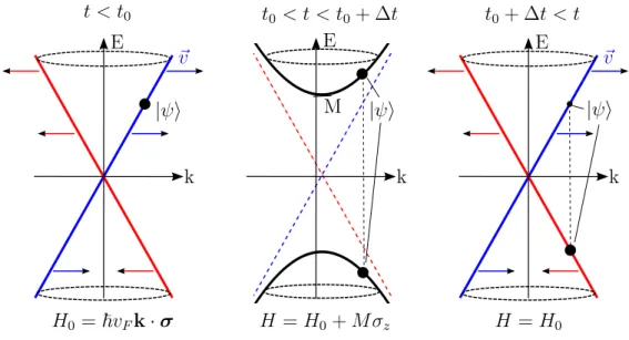
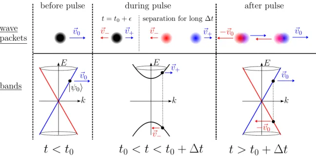
The linear band structure of graphene in vicinity of itsK- andK⁰-points is beneficial for the sake of echoes due to two features. One feature is the constant magnitude of the phase velocity v_F and the other even more important one is its chiral symmetry implying negative velocity of the valence band (E <0) as compared to the conduction band (E >0). For this reason, our goal will be to revert the population of the two bands by a pulse. The velocity after the pulse has the same magnitude v_F, but points in the opposite direction as compared to before. Thus a perfect echo of the initial state is achieved – provided perfect population inversion.

The initial Hamiltonian we use is an effective low-energy Hamiltonian around the K-point given by the massless Dirac equation in 2d, compare Sec. 2.1.1,

H₀ =~v_F k·σ =~v_F

0 k_x−ik_y k_x+ik_y 0

(3.1) Note that for graphene, the Pauli matricesσ_i are operators in the pseudospin space.

The additional degeneracy of spins is not of importance for the basic principle of the echo and therefore not considered.

Since k is a good quantum number, the eigenenergies and eigenvectors can be labeled by kand a band index s=±:

E_k,s =s~v_Fk =:s E_k, (3.2)

hk|ϕk,si= 1

√2 1

se^iγ^k

, (3.3)

where k = |k| and γ_k is the polar angle in reciprocal space. An important feature is that for every k, the eigenstates|ϕ_k,si are complete in pseudospin space meaning that

X

s

|ϕ_k,sihϕ_k,s|=|kihk|1ps (3.4) with 1ps being the unit operator in pseudospin space.

Since the Hamiltonian in Eq. (3.3) is not only immanent to graphene, other systems whose time propagation is described by the same Hamiltonian can be used for this echo mechanism, like artificial graphene or Dirac plasmons. Moreover, the

(25)

3.Dirac Quantum Time Mirror

~ v M

~v

k E

|ψi

k E

|ψi

k E

|ψi t₀ < t < t₀+ ∆t

t < t₀ t₀+ ∆t < t

H₀ =~v_Fk·σ H =H₀+M σ_z H =H₀

Figure 3.1: Transition mechanism in graphene for an exemplary initial state |ψi, induced by opening a band gap. The band structure before, during and after the pulse is shown. Due to the linear band structure, the magnitude of the group velocity is constant, but the direction is opposite in the blue band and in the red band, indicated by the colored arrows. Before the pulse, the initial state is in the blue band and moves therefore to the right. During the pulse, a band gap opens and the initial state is not in an eigenstate of the Hamiltonian anymore but in a superposition of the two new eigenstates, which oscillate with different frequencies.

Depending on the pulse strength M and the pulse duration ∆t, the state switches partly to the other band (red branch). Due to the opposite velocity, this part of the state goes after the pulse back to its initial position as an echo.

exact coupling between the (pseudospin) and momentum is not important. The same echo mechanism also works for 3D topological insulator surface states, which can be described byH_TI=~v_Fk·(σ×eˆ_z) [78], whose band structure is also linear.

The only difference is the pseudospin orientation of the energy-eigenstates, which is not relevant, since a unitary rotation of the spin-space maps one Hamiltonian in the other. Nevertheless, to avoid confusion, we will consider only graphene henceforth, but all results also apply to the afore mentioned systems.

Again, to stress the main mechanism of our proposed quantum time mirror (QTM), the echo is achieved by inverting the energy, but keeping the momentum k fixed, as can be seen in Fig. 3.1. In consequence, the direction of the velocity of every mode is also inverted (v→ −v) due to the peculiar band structure.

The transition is induced by a time-dependent Hamiltonian H₁(t), which is chosen to be nonzero only fort₀ < t < t₀+ ∆t wheret₀ is the time of the pulse and ∆t is the pulse duration. The full Hamiltonian during the pulse is H(t) =H0+H1(t) and the time evolution operator U becomes

U(t₀, t₀+ ∆t) =T exp

−i/~

Z t0+∆t t0

H(t) dt

, (3.5)

withT denoting the time-ordered product, resp. the time-ordered exponential. For

(26)

3.1. Echo mechanism and transition amplitude

simplicity, we choose

H₁(t) =

M , tˆ ₀ < t < t₀ + ∆t,

0, otherwise, (3.6)

meaning that the pulse is switched on and off abruptly to a constant potential ˆM, which is homogeneous in space. This simplifies the time evolution operator during the pulse, getting rid of the time ordered exponential

U(t₀, t₀+ ∆t) = exp

−i

~

(H₀+ ˆM)∆t

. (3.7)

Note that the restriction of abrupt switching of the pulse is not a necessary condition for the echo. Qualitatively the same results for other pulse shapes, as long as it is fast enough (diabatic) compared to the other energies in the system, e.g.

the pulse strength or the energy of the wave packet. Moreover, since H(t) is not space-dependent,kis still a good quantum number, i.e. the momentum operator~ˆk commutes with H, but energy is not conserved due to the time-dependence.

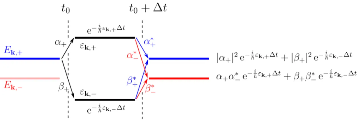
A perfect occupation inversion of the bands is achieved ifU(t₀, t₀+ ∆t) maps an eigenstate at konto the eigenstate with negative energy and the same k:

U(t0, t0+ ∆t)|ϕk,±i=α|ϕk,∓i, α∈C, |α|² = 1. (3.8) Because of this condition, it is reasonable to choose ˜M =M σ_z. Due to the structure of the eigenstates in Eq. (3.3), we see that σ_z serves the purpose

σ_z|ϕk,±i=|ϕk,∓i, (3.9)

since σ_z only changes the sign of the second component of the spinor. Physically, M σ_z is an effective mass term in the Dirac equation, which opens a gap. The full Hamiltonian reads:

H =H₀ +H₁ =~v_Fk·σ+f(t)M σ_z, with f(t) =

1, t₀ < t < t₀+ ∆t, 0, otherwise.

(3.10) The eigenvalues and eigenvectors of H during the pulse become

εk,± =± q

M²+~²v_F²k² =±M√

1 +κ², (3.11)

hk|χk,±i= 1

p(M +εk,±)²+~²v_F²k²

M +εk,±

~v_Fke^iγ^k

= 1

√2p

1 +κ²±√ 1 +κ²

1±√ 1 +κ² κe^iγ^k

. (3.12)

Here we introduced the dimensionless quantity κ= ~v_Fk

M , (3.13)

which is the ratio between the energy of a mode without perturbation and the gap width and is therefore an inverse, relative measure for the pulse strength.