Construction of the Z-Order Curve in 3D
1.
Choose a level k
2.
Construct a regular lattice of points in the unit cube, 2
kpoints along each dimension
3.
Represent the coordinates of a lattice point p by integer/binary number, i.e., k bits for each coordinate, p
x= b
x,k…b
x,14.
Define the Morton code of p as the interleaved bits of the coordinates, i.e., m(p) = b
z,kb
y,kb
x,k…b
z,1b
y,1b
x,15.
Connect the points in the order of their Morton codes
⟶z-order curve at level k
Example
11
10
01
00
00 01 10 11
y x y x
0000
lowest level
1010 1011 1110 1111
1000 1001 1110 1101
0010 0011 0110 0111
0000 0001 0100 0101
Note: the Z-curve induces a grid (actually, a multi-grid)
1010 1011 1110 1111
1000 1001 1110 1101
0010 0011 0110 0111
0000 0001 0100 0101
11
10
01
00
00
Properties of Morton Codes
§ The Morton code of each point is 3k bits long
§ All points p with Morton code m(p) = 0xxx lie below the plane z=1/2
§ All points with m(p) = 111xxx lie in the upper right quadrant of the cube
§ If we build a binary tree/quadtree/octree on top of the grid, then the Morton code encodes the
path of a point, from the root to the leaf thatcontains the point ("0" = left, "1" = right)
§ The Morton codes of two points differ
for the first time – when read from left to right – at bit position h
⇔the paths in the binary tree over the grid split at level h
0010
Construction of Linear BVHs
§ Scale all polygons such that bbox = unit cube
§ Replace polygons by their "center point"
§ E.g., center point = barycenter (Schwerpunkt), or center point = center of bbox of polygon
0.0 1.0
1.0
§ Assign Morton codes to points according to enclosing grid cell
§ Assign those Morton codes to the original polygons, too
1010 1011 1110 1111
1000 1001 1110 1101
0010 0011 0110 0111
0000 0001 0100 0101
§ Now, we've got a list of pairs of ⟨polygon ID, Morton code⟩
§ Example:
§
Sort list according to Morton code, i.e., along z-curve⟶
linearization
§ Next: find index intervals representing BVH nodes at different levels
0000
0010 0011
1000 1001
1010 1110 1101
0000 0010 0011 1000 1001 1010 1110 1101
Pgon ID ⟶ Morton code ⟶
Array index i ⟶ 0 1 2 3 4 5 6 7 Pgon ID ⟶
Morton code ⟶
§ Now, root of BVH = polygons in index range 0,…,N-1
§ All polygons with first bit of Morton code = 0/1 are below/above the plane z = 1/2
§ Find index i in sorted array where first bit (MSB) changes from "0" to "1"
§ Left child of root = polygons in index range 0,…,i-1
§ Right child of root = polygons in index range i,…,N-1
§ In general (recursive formulation):
§ Given: level h, and index range i,…,j in sorted array, such that Morton codes are identical for all polygons in that range up to bit h
§ Find index k in [i,j] where the bit at position h' (h' > h) in Morton codes changes from "0" to "1"
§ Can be achieved quickly by binary search and CUDA's __clz()
function (= "count number of leading zeros")
§ Consider polygon i and i+1 in the array
§ Condition for "same node":
Polygons i and i+1 are in the same node of the BVH at level h
⇔Morton codes are the same up to bit h
§ Define a split marker := ⟨index i, level h⟩
§ Parallel computation of all split markers
⟶"split list":
§ Each thread i checks polygons i and i+1
§ Loop over their Morton codes, let h be left-most bit position where the two Morton codes differ
§ Output split markers ⟨i,h⟩, …, ⟨i,3k⟩ (seems like a bit of overkill)
§ Can be at most 3k split markers per thread ⟶ static memory allocations works
§ Example:
0000 0010 0011 1000 1001 1010 1110 1101
Pgon ID ⟶ Morton code ⟶
Array index i ⟶ 0 1 2 3 4 5 6 7
(0,3) (1,4) (4,3) (5,2) (6,4)
(0,4) (4,4) (5,3)
(5,4) (3,4)
(2,1) (2,2) (2,3) (2,4)
Split pair = (i,h) , i ∈ [0,N-2] , h ∈ [1,3k]
§ Last step:
§ Compact split list
§ Sort split list by level h
§ Must be stable sort!
§ For each level h, we now have ranges of indices in the resulting
list; all primitives within a range are in the same node on that
level h
§ Example:
§ Final steps:
§ Remove singleton BVH nodes
§ Compute bounding boxes for each node/interval
§ Convert to "regular" BVH with pointers
§ Limitations:
§ Not optimized for ray tracing
§ Morton code only approximates locality
Faster Ray-Tracing by Sorting
§ Recap: the principle of ray-tracing
§ Shoot one (or many) primary rays per pixel into the scene
§ Find first intersection (accelerate by, e.g., 3D grid)
§ Generate secondary rays (in order to collect light from all different directions)
§ Recursion ⟶ ray tree
§ Ray-Tracing is "embarrassingly parallel":
§ Just start one thread per primary ray
§ Or, is it that simple?
§ Visualization of the principle and the work flow:
Reflection Rays Shadow Rays
§ The ray tree for one primary ray:
§ Problem for massive parallelization:
§ Each thread traverses their own ray tree
§ The rays each thread currently follows go in all kinds of different directions
§ Consequence: thread divergence!
§ Another problem: each thread needs their own stack!
G. Zachmann Massively Parallel Algorithms SS 9 July 2014 Sorting 85
§ Definition coherent rays:
Two rays that have "approximately" the same origin and the same direction are said to be coherent rays.
A set of coherent rays is sometimes called a coherent ray packet.
§ Observations:
§ Coherent rays are likely to hit the same object in the scene
§ Coherent rays will likely hit the same cells in an acceleration data structure (e.g., grid or kd-tree)
Kirill Garanzha & Charles Loop / Fast Ray Sorting and Breadth-First Packet Traversal for GPU Ray Tracing
We then perform data compaction into Chunk Base and Chunk Hash arrays: for each Head Flags
i= 1 we write the value i into position of Chunk Base array specified by Scan(Head Flags)
i. Analogously, we build Chunk Hash array. The values of Chunk Size elements are equal to dif- ferences between neighboring Chunk Base elements.
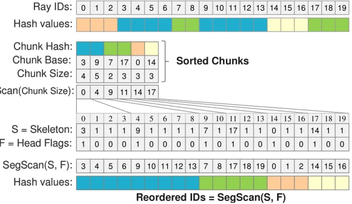
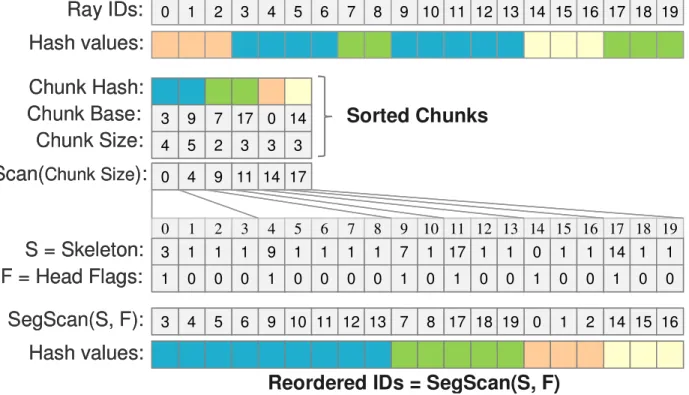
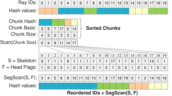
Decompression. When the compressed data is sorted we apply an exclusive scan procedure to the Chunk Size array (see Fig. 5). We initialize the array Skeleton with ones, and the array Head Flags with zeroes (the sizes of both arrays are equal to Hash values array). Into positions of the array Skeleton specified by Scan(Chunk Size) we write the cor- responding values of Chunk Base array. Into positions of the array Head Flags specified by Scan(Chunk Size) we write ones. We then apply an inclusive segmented scan [SHG08] to array Skeleton considering the Head Flags array that specifies the bounds of data segments. The result of the segmented scan is the array of reordered (sorted) ray ids corresponding to their hash values.
0 1 2 3 4 5 6 7 8 9 10 11 12 13 14 15 16 17 18 19 0
3 9 7 17 14 3
4 5 2 3 3
Scan(Chunk Size): 0 4 9 11 14 17
3 1 1 1 9 1 1 1 1 7 1 17 1 1 0 1 1 14 1 1
S = Skeleton:
0 1 2
3 4 5 6 9 10 11 12 13 7 8 17 18 19 14 15 16
SegScan(S, F):
1 0 0 0 1 0 0 0 0 1 0 1 0 0 1 0 0 1 0 0
F = Head Flags:
Hash values:
0 1 2 3 4 5 6 7 8 9 10 11 12 13 14 15 16 17 18 19
Ray IDs:
Hash values:
Chunk Base:
Chunk Size:
Chunk Hash:
Sorted Chunks
Reordered IDs = SegScan(S, F)
Figure 5: Decompression example.
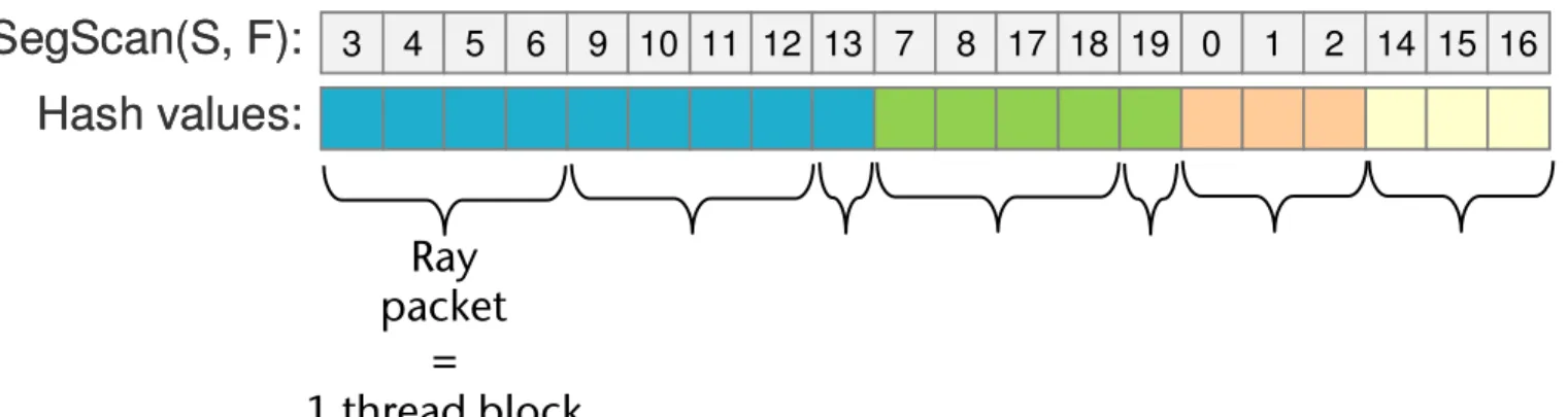
Decomposition: packet ranges extraction. We would like to create packets of coherent rays no larger than some capacity (e.g., MaxSize = 256). First, we extract the base index and range of each cell that contains the chunk of rays with the same hash value. In order to do this we apply the compression procedure described above to the array of sorted rays. As a result each element of Chunk Size repre- sents the number of rays assigned to the corresponding grid cell (see Fig. 6).
0 1 2 3 4 5 6
Chunk Base:
Chunk Size:
Chunk Hash:
0 9 3
9 5 3
numPackets: 3 2 1 1
0 4 4 9 4
S = Skeleton:
0 4 8 9 14 17
SegScan(S, F):
1 0 0 1 0 1 1
F = Head Flags:
14 17
Scan(numPackets): 0 3 5 6
14 17
13
Ray Packet Base = SegScan(S, F)
0 1 2 3 4 5 6
Chunk Base:
Chunk Size:
Chunk Hash:
0 9 3
9 5 3
numPackets: 3 2 1 1
0 4 4 9 4
S = Skeleton:
0 4 8 9 14 17
SegScan(S, F):
1 0 0 1 0 1 1
F = Head Flags:
14 17
Scan(numPackets): 0 3 5 6
14 17
13
Ray Packet Base = SegScan(S, F)
Figure 6: Decomposition example. On this example each chunk is decomposed into the packets of MaxSize = 4.
We create the array numPackets where numPackets
i= (ChunkSize
i+ MaxSize – 1) / MaxSize and then scan this array. All the values of Skeleton are initially set to MaxSize and all values of Head Flags are set to zero. Into positions of the array Skeleton specified by Scan(numPackets) we write the corresponding values of array Chunk Base. Into positions of the array Head Flags specified by Scan(numPackets) we write ones. As in the decompression procedure, we apply an inclusive segmented scan to array Skeleton considering the Head Flags. The result of this segmented scan is the array of base indices for each ray packet, the size of a ray packet is found as the difference of consecutive bases.
3.2 Frustum Creation
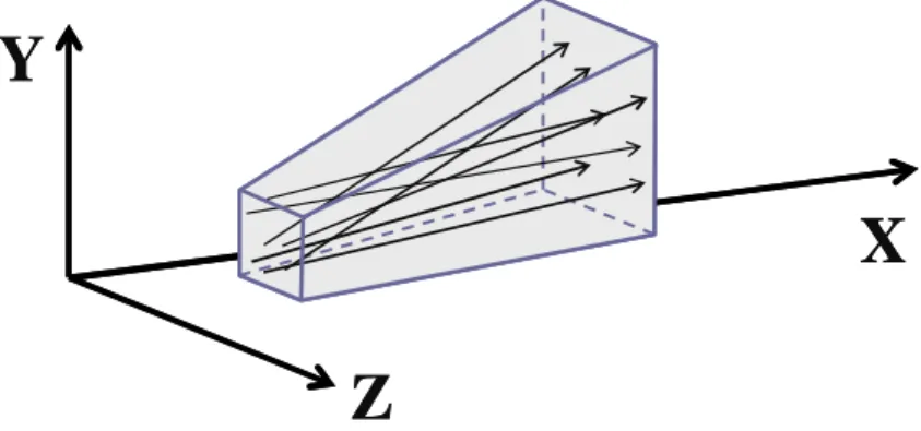
Once the rays are sorted and packet ranges extracted, we build a frustum for each packet. As in the work [ORM08], we define the frustum by using a dominant axis and two axis-aligned rectangles. The dominant axis corresponds to the ray direction component with a maximum absolute value. For the coherent rays of a packet this axis is assumed to be the same. The two axis-aligned rectangles are perpendicular to this dominant axis and bound all the rays of the packet (see Fig. 7).
X Y
Z
X Y
Z
Figure 7: Frustum is defined by dominant axis X and two axis-aligned rectangles.
We implemented the frustum creation in a single CUDA kernel where each frustum is computed by a warp of (32) threads. Shared memory is used to compute the valid in- terval along the dominant axis and base rectangles for all the rays in a packet.
3.3 Breadth-First Frustum Traversal
We perform breadth-first frustum traversal through the BVH with the arity equal to eight. The binary BVH is constructed on the CPU and 2/3
rdsof tree levels are eliminated and an Octo-BVH is created (all the nodes are stored in a breadth-first storage layout). Each BVH-node is represented with 32 bytes: six float values for the axis- aligned bounding box (AABB), one 32-bit integer value represents the block of children (3 bytes for the base offset of the block and 1 byte for the number of children), and one 32-bit integer for the spatial order of children within this node. All the children within the node are sorted in a spatial 3D ascending order (see Fig. 8).
Per frustum child ordering. For each frustum, a 3-bit
value of F(DirSigns) is computed that corresponds to the
sign bits of the average frustum’s ray direction. The spatial
order of node’s children along the frustum direction is
Approach to Solve the Divergence Problem
§ Take a stream of rays as input
§ Can be arbitrary mix of primary, secondary, tertiary, shadow rays, …
§ Arrange them into packets of coherent rays
§ Compute ray-scene intersections
§ One thread per ray
§ Each block of threads processes one coherent ray packet
§ Each thread traverses the acceleration data structure
§ At the end of this procedure, each thread generates a number of new rays In the following, we will look at this step
G. Zachmann Massively Parallel Algorithms SS 9 July 2014 Sorting 87
Identifying Coherent Rays
§ General approach: classification by discretization
§ Here: compute a (trivial) hash value per ray
§ Discretize the ray origin by a 3D grid ⟶ first part of hash value
§ Discretize ray direction by direction cube ⟶ second part
§ Concatenate the two hash parts ⟶ complete hash value
§ Can be done in parallel for each ray:
Kirill Garanzha & Charles Loop / Fast Ray Sorting and Breadth-First Packet Traversal for GPU Ray Tracing
CUDA) that is slower than shared memory since it is mapped to global GPU memory [NVIDIA]. Several works [HSHH07;
GPSS07] described ways to eliminate or miti-gate stack usage in a GPU ray tracer. But these approaches have no solution for the warp-wise multi-branching prob- lem that was analyzed by Aila and Laine [AL09]. This problem was mitigated by using persistent threads that fetch the ray tracing task per each idle warp of threads.
Some warps within a block of threads become idle if one warp executes longer than others. In our ray tracing pipe- line we eliminate this warp-wise multi-branching at ex- pense of a long pipeline and special ray sorting. Roger et al. [RAH07] presented a GPU ray-space hierarchy con- struction process based on screen-space indexing. Rays were not actually sorted for better coherence.
3. GPU Ray Tracing Pipeline
In order to map ray tracing to efficient GPU execution we decompose ray tracing into 4 stages: ray sorting, frustum creation, breadth-first traveral, and localized ray-primitive intersections (see Fig. 1).
Ray sorting is used to store spatially coherent rays in consecutive memory locations. Compared to unsorted rays, the tracing routine for sorted rays has less divergence on a wide SIMD machine such as GPU. Extracting packets of coherent rays enables tight frustum creation for packets of rays. We explicitly maintain ray coherence in our pipeline by using this procedure.
We create tight frustums in order to traverse the BVH using only frustums instead of individual rays. For each frustum we build the spatially sorted list of BVH-leaves that are intersected by the frustum. Given that the set of frustums is much smaller than the set of rays, we perform breadth-first frustum traversal utilizing a narrower parallel scan per each BVH level.
In the localized ray-primitive intersection stage, each ray that belongs to the frustum is tested against all the primi- tives contained in a list of sorted BVH-leaves captured in a previous stage.
3.1 Ray Sorting
Our ray sorting procedure is used to accelerate ray tracing by extracting coherence and reducing execution branches within a SIMD processor. However, the cost of such ray sorting should be offset by an increase in performance. We propose a technique that is based on compression of key- index pairs. Then we sort the compressed sequence and decompress the sorted data.
Ray hash. We create the sequence of key-index pairs by
using the ray id as index, and a hash value computed for this ray as the key. We quantize the ray origins assuming a virtual uniform 3D-grid within scene’s bounding box. We also quantize normalized ray directions assuming a virtual
uniform grid (see
Fig. 2). We manually specify the cellsizes for both virtual grids (see section 5.1). With quan- tized components of the origin and direction we compute cell ids within these grids and merge them into a 32-bit hash value for each ray. Rays that map to the same hash value are considered to be coherent in the 3D-space.
0 1 2 3 4 5 6 7
0 1 2 3
1 0
2 3 4
5 6
7
0 1 2 3 4 5 6 7
0 1 2 3
1 0
2 3 4
5 6
7
1 0
2 3 4
5 6
7
Figure 2: The quantization of ray origin and direction is used to compute a hash value for a given ray.
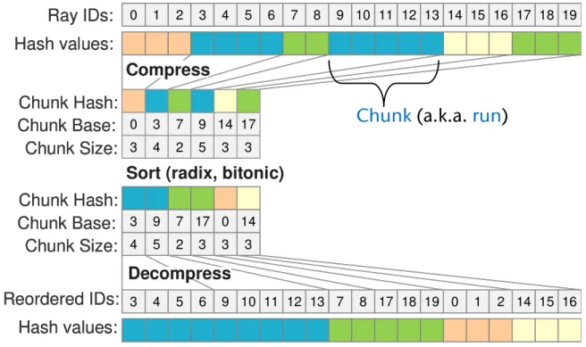
Sorting. We introduce a “compression – sorting – de-
compression” (CSD) scheme (see
Fig. 3) and explicitlymaintain coherence through all the ray bounce levels. Co- herent rays hit similar geometry locations. And these hit points form ray origins for next-generation rays (bounced rays). There is a non-zero probability that some sequen- tially generated rays will receive the same hash value. This observation is exploited and sorting becomes faster. The compressed ray data is sorted using radix sort [SHG09].
0 1 2 3 4 5 6 7 8 9 10 11 12 13 14 15 16 17 18 19
Ray IDs:
Hash values:
0 3 7 9 14 17 3 4 2 5 3 3
Chunk Base:
Chunk Size:
Chunk Hash:
Chunk Base:
Chunk Size:
Chunk Hash:
0 3 9 7 17 14
3
4 5 2 3 3
0 1 2
3 4 5 6 9 10 11 12 13 7 8 17 18 19 14 15 16
Reordered IDs:
Hash values:
Decompress Compress
Sort (radix, bitonic)
Figure 3: The overall ray sorting scheme.
Compression. We create the array Head Flags equal in
size to the array
Hash values. All the elements of Head Flags are set to 0 except for the elements whose corres-ponding hash value is not equal to the previous one (see
Fig. 4). We apply an exclusive scan procedure [SHG08] tothe Head Flags array.
0 1 2 3 4 5
0 1 2 3 4 5 6 7 8 9 10 11 12 13 14 15 16 17 18 19
Ray IDs:
Hash values:
0 3 7 9 14 17 3 4 2 5 3 3
Chunk Base:
Chunk Size:
Chunk Hash:
1 0 0 1 0 0 0 1 0 1 0 0 0 0 1 0 0 1 0 0
Head Flags:
0 1 1 1 2 2 2 2 3 3 4 4 4 4 4 5 5 5 6 6
Scan(Head Flags):
0 1 2 3 4 5
0 1 2 3 4 5 6 7 8 9 10 11 12 13 14 15 16 17 18 19
Ray IDs:
Hash values:
0 3 7 9 14 17 3 4 2 5 3 3
Chunk Base:
Chunk Size:
Chunk Hash:
1 0 0 1 0 0 0 1 0 1 0 0 0 0 1 0 0 1 0 0
Head Flags:
0 1 1 1 2 2 2 2 3 3 4 4 4 4 4 5 5 5 6 6
Scan(Head Flags):
Figure 4: Compression example.
Kirill Garanzha & Charles Loop / Fast Ray Sorting and Breadth-First Packet Traversal for GPU Ray Tracing
© 2009 The Author(s)
Journal compilation © 2009 The Eurographics Association and Blackwell Publishing Ltd.
CUDA) that is slower than shared memory since it is mapped to global GPU memory [NVIDIA]. Several works [HSHH07; GPSS07] described ways to eliminate or miti- gate stack usage in a GPU ray tracer. But these approaches have no solution for the warp-wise multi-branching prob- lem that was analyzed by Aila and Laine [AL09]. This problem was mitigated by using persistent threads that fetch the ray tracing task per each idle warp of threads.
Some warps within a block of threads become idle if one warp executes longer than others. In our ray tracing pipe- line we eliminate this warp-wise multi-branching at ex- pense of a long pipeline and special ray sorting. Roger et al. [RAH07] presented a GPU ray-space hierarchy con- struction process based on screen-space indexing. Rays were not actually sorted for better coherence.
3. GPU Ray Tracing Pipeline
In order to map ray tracing to efficient GPU execution we decompose ray tracing into 4 stages: ray sorting, frustum creation, breadth-first traveral, and localized ray-primitive intersections (see Fig. 1).
Ray sorting is used to store spatially coherent rays in consecutive memory locations. Compared to unsorted rays, the tracing routine for sorted rays has less divergence on a wide SIMD machine such as GPU. Extracting packets of coherent rays enables tight frustum creation for packets of rays. We explicitly maintain ray coherence in our pipeline by using this procedure.
We create tight frustums in order to traverse the BVH using only frustums instead of individual rays. For each frustum we build the spatially sorted list of BVH-leaves that are intersected by the frustum. Given that the set of frustums is much smaller than the set of rays, we perform breadth-first frustum traversal utilizing a narrower parallel scan per each BVH level.
In the localized ray-primitive intersection stage, each ray that belongs to the frustum is tested against all the primi- tives contained in a list of sorted BVH-leaves captured in a previous stage.
3.1 Ray Sorting
Our ray sorting procedure is used to accelerate ray tracing by extracting coherence and reducing execution branches within a SIMD processor. However, the cost of such ray sorting should be offset by an increase in performance. We propose a technique that is based on compression of key- index pairs. Then we sort the compressed sequence and decompress the sorted data.
Ray hash. We create the sequence of key-index pairs by using the ray id as index, and a hash value computed for this ray as the key. We quantize the ray origins assuming a virtual uniform 3D-grid within scene’s bounding box. We also quantize normalized ray directions assuming a virtual
uniform grid (see Fig. 2). We manually specify the cell sizes for both virtual grids (see section 5.1). With quan- tized components of the origin and direction we compute cell ids within these grids and merge them into a 32-bit hash value for each ray. Rays that map to the same hash value are considered to be coherent in the 3D-space.
0 1 2 3 4 5 6 7
0 1 2 3
1 0
2 3 4
5 6
7
0 1 2 3 4 5 6 7
0 1 2 3
1 0
2 3 4
5 6
7
1 0
2 3 4
5 6
7
Figure 2: The quantization of ray origin and direction is used to compute a hash value for a given ray.
Sorting. We introduce a “compression – sorting – de- compression” (CSD) scheme (see Fig. 3) and explicitly maintain coherence through all the ray bounce levels. Co- herent rays hit similar geometry locations. And these hit points form ray origins for next-generation rays (bounced rays). There is a non-zero probability that some sequen- tially generated rays will receive the same hash value. This observation is exploited and sorting becomes faster. The compressed ray data is sorted using radix sort [SHG09].
0 1 2 3 4 5 6 7 8 9 10 11 12 13 14 15 16 17 18 19
Ray IDs:
Hash values:
0 3 7 9 14 17 3 4 2 5 3 3
Chunk Base:
Chunk Size:
Chunk Hash:
Chunk Base:
Chunk Size:
Chunk Hash:
0 3 9 7 17 14
3
4 5 2 3 3
0 1 2
3 4 5 6 9 10 11 12 13 7 8 17 18 19 14 15 16
Reordered IDs:
Hash values:
Decompress Compress
Sort (radix, bitonic)
Figure 3: The overall ray sorting scheme.
Compression. We create the array Head Flags equal in size to the array Hash values. All the elements of Head Flags are set to 0 except for the elements whose corres- ponding hash value is not equal to the previous one (see Fig. 4). We apply an exclusive scan procedure [SHG08] to the Head Flags array.
0 1 2 3 4 5
0 1 2 3 4 5 6 7 8 9 10 11 12 13 14 15 16 17 18 19
Ray IDs:
Hash values:
0 3 7 9 14 17 3 4 2 5 3 3
Chunk Base:
Chunk Size:
Chunk Hash:
1 0 0 1 0 0 0 1 0 1 0 0 0 0 1 0 0 1 0 0
Head Flags:
0 1 1 1 2 2 2 2 3 3 4 4 4 4 4 5 5 5 6 6
Scan(Head Flags):
0 1 2 3 4 5
0 1 2 3 4 5 6 7 8 9 10 11 12 13 14 15 16 17 18 19
Ray IDs:
Hash values:
0 3 7 9 14 17 3 4 2 5 3 3
Chunk Base:
Chunk Size:
Chunk Hash:
1 0 0 1 0 0 0 1 0 1 0 0 0 0 1 0 0 1 0 0
Head Flags:
0 1 1 1 2 2 2 2 3 3 4 4 4 4 4 5 5 5 6 6
Scan(Head Flags):
Figure 4: Compression example.
§ Note: often, there are many consecutive rays (in the input array) that are coherent, i.e., will map to the same ray hash value
§ For instance, shadow rays
§ Multiple secondary rays from glossy surfaces, etc.
G. Zachmann Massively Parallel Algorithms SS 9 July 2014 Sorting 89
§ Can we sort the array of rays yet?
§ We could, but we'd perform way too much work!
§ Idea:
1. Compact the array
- Similar to run length compression/coding
2. Sort 3. Unpack
Kirill Garanzha & Charles Loop / Fast Ray Sorting and Breadth-First Packet Traversal for GPU Ray Tracing
CUDA) that is slower than shared memory since it is mapped to global GPU memory [NVIDIA]. Several works [HSHH07; GPSS07] described ways to eliminate or miti- gate stack usage in a GPU ray tracer. But these approaches have no solution for the warp-wise multi-branching prob- lem that was analyzed by Aila and Laine [AL09]. This problem was mitigated by using persistent threads that fetch the ray tracing task per each idle warp of threads.
Some warps within a block of threads become idle if one warp executes longer than others. In our ray tracing pipe- line we eliminate this warp-wise multi-branching at ex- pense of a long pipeline and special ray sorting. Roger et al. [RAH07] presented a GPU ray-space hierarchy con- struction process based on screen-space indexing. Rays were not actually sorted for better coherence.
3. GPU Ray Tracing Pipeline
In order to map ray tracing to efficient GPU execution we decompose ray tracing into 4 stages: ray sorting, frustum creation, breadth-first traveral, and localized ray-primitive intersections (see Fig. 1).
Ray sorting is used to store spatially coherent rays in consecutive memory locations. Compared to unsorted rays, the tracing routine for sorted rays has less divergence on a wide SIMD machine such as GPU. Extracting packets of coherent rays enables tight frustum creation for packets of rays. We explicitly maintain ray coherence in our pipeline by using this procedure.
We create tight frustums in order to traverse the BVH using only frustums instead of individual rays. For each frustum we build the spatially sorted list of BVH-leaves that are intersected by the frustum. Given that the set of frustums is much smaller than the set of rays, we perform breadth-first frustum traversal utilizing a narrower parallel scan per each BVH level.
In the localized ray-primitive intersection stage, each ray that belongs to the frustum is tested against all the primi- tives contained in a list of sorted BVH-leaves captured in a previous stage.
3.1 Ray Sorting
Our ray sorting procedure is used to accelerate ray tracing by extracting coherence and reducing execution branches within a SIMD processor. However, the cost of such ray sorting should be offset by an increase in performance. We propose a technique that is based on compression of key- index pairs. Then we sort the compressed sequence and decompress the sorted data.
Ray hash. We create the sequence of key-index pairs by using the ray id as index, and a hash value computed for this ray as the key. We quantize the ray origins assuming a virtual uniform 3D-grid within scene’s bounding box. We also quantize normalized ray directions assuming a virtual
uniform grid (see Fig. 2). We manually specify the cell sizes for both virtual grids (see section 5.1). With quan- tized components of the origin and direction we compute cell ids within these grids and merge them into a 32-bit hash value for each ray. Rays that map to the same hash value are considered to be coherent in the 3D-space.
0 1 2 3 4 5 6 7
0 1 2 3
1 0
2 3 4 5 6
7
0 1 2 3 4 5 6 7
0 1 2 3
1 0
2 3 4 5 6
7
1 0
2 3 4 5 6
7
Figure 2: The quantization of ray origin and direction is used to compute a hash value for a given ray.
Sorting. We introduce a “compression – sorting – de- compression” (CSD) scheme (see Fig. 3) and explicitly maintain coherence through all the ray bounce levels. Co- herent rays hit similar geometry locations. And these hit points form ray origins for next-generation rays (bounced rays). There is a non-zero probability that some sequen- tially generated rays will receive the same hash value. This observation is exploited and sorting becomes faster. The compressed ray data is sorted using radix sort [SHG09].
0 1 2 3 4 5 6 7 8 9 10 11 12 13 14 15 16 17 18 19
Ray IDs:
Hash values:
0 3 7 9 14 17 3 4 2 5 3 3
Chunk Base:
Chunk Size:
Chunk Hash:
Chunk Base:
Chunk Size:
Chunk Hash:
0 3 9 7 17 14
3
4 5 2 3 3
0 1 2
3 4 5 6 9 10 11 12 13 7 8 17 18 19 14 15 16
Reordered IDs:
Hash values:
Decompress Compress
Sort (radix, bitonic)
0 1 2 3 4 5 6 7 8 9 10 11 12 13 14 15 16 17 18 19
Ray IDs:
Hash values:
0 3 7 9 14 17 3 4 2 5 3 3
Chunk Base:
Chunk Size:
Chunk Hash:
Chunk Base:
Chunk Size:
Chunk Hash:
0 3 9 7 17 14
3
4 5 2 3 3
0 1 2
3 4 5 6 9 10 11 12 13 7 8 17 18 19 14 15 16
Reordered IDs:
Hash values:
Decompress Compress
Sort (radix, bitonic)
Figure 3: The overall ray sorting scheme.
Compression. We create the array Head Flags equal in size to the array Hash values. All the elements of Head Flags are set to 0 except for the elements whose corres- ponding hash value is not equal to the previous one (see Fig. 4). We apply an exclusive scan procedure [SHG08] to the Head Flags array.
0 1 2 3 4 5
0 1 2 3 4 5 6 7 8 9 10 11 12 13 14 15 16 17 18 19
Ray IDs:
Hash values:
0 3 7 9 14 17 3 4 2 5 3 3
Chunk Base:
Chunk Size:
Chunk Hash:
1 0 0 1 0 0 0 1 0 1 0 0 0 0 1 0 0 1 0 0
Head Flags:
0 1 1 1 2 2 2 2 3 3 4 4 4 4 4 5 5 5 6 6
Scan(Head Flags):
0 1 2 3 4 5
0 1 2 3 4 5 6 7 8 9 10 11 12 13 14 15 16 17 18 19
Ray IDs:
Hash values:
0 3 7 9 14 17 3 4 2 5 3 3
Chunk Base:
Chunk Size:
Chunk Hash:
1 0 0 1 0 0 0 1 0 1 0 0 0 0 1 0 0 1 0 0
Head Flags:
0 1 1 1 2 2 2 2 3 3 4 4 4 4 4 5 5 5 6 6
Scan(Head Flags):
Figure 4: Compression example.
Chunk (a.k.a. run)
G. Zachmann Massively Parallel Algorithms SS 9 July 2014 Sorting 90
Ray Array Compaction
1.
Set all
HeadFlags[i] = 1, where
HashValue[i-1] ≠ HashValue[i], else set
HeadFlag[i] = 02.
Apply exclusive prefix sum to
HeadFlagsarray
⟶ ScanHeadFlags§ Now, ScanHeadFlags[i] contains new position in the Chunk arrays
3.
For all i, where
HeadFlags[i]==1:
ChunkBase[ ScanHeadFlags[i] ] = i
ChunkHash[ ScanHeadFlags[i] ] = HashValue[i]
4.
Set all
ChunkSize[i] = ChunkBase[i+1]
– ChunkBase[i]
Kirill Garanzha & Charles Loop / Fast Ray Sorting and Breadth-First Packet Traversal for GPU Ray Tracing
CUDA) that is slower than shared memory since it is mapped to global GPU memory [NVIDIA]. Several works [HSHH07; GPSS07] described ways to eliminate or miti- gate stack usage in a GPU ray tracer. But these approaches have no solution for the warp-wise multi-branching prob- lem that was analyzed by Aila and Laine [AL09]. This problem was mitigated by using persistent threads that fetch the ray tracing task per each idle warp of threads.
Some warps within a block of threads become idle if one warp executes longer than others. In our ray tracing pipe- line we eliminate this warp-wise multi-branching at ex- pense of a long pipeline and special ray sorting. Roger et al. [RAH07] presented a GPU ray-space hierarchy con- struction process based on screen-space indexing. Rays were not actually sorted for better coherence.
3. GPU Ray Tracing Pipeline
In order to map ray tracing to efficient GPU execution we decompose ray tracing into 4 stages: ray sorting, frustum creation, breadth-first traveral, and localized ray-primitive intersections (see Fig. 1).
Ray sorting is used to store spatially coherent rays in consecutive memory locations. Compared to unsorted rays, the tracing routine for sorted rays has less divergence on a wide SIMD machine such as GPU. Extracting packets of coherent rays enables tight frustum creation for packets of rays. We explicitly maintain ray coherence in our pipeline by using this procedure.
We create tight frustums in order to traverse the BVH using only frustums instead of individual rays. For each frustum we build the spatially sorted list of BVH-leaves that are intersected by the frustum. Given that the set of frustums is much smaller than the set of rays, we perform breadth-first frustum traversal utilizing a narrower parallel scan per each BVH level.
In the localized ray-primitive intersection stage, each ray that belongs to the frustum is tested against all the primi- tives contained in a list of sorted BVH-leaves captured in a previous stage.
3.1 Ray Sorting
Our ray sorting procedure is used to accelerate ray tracing by extracting coherence and reducing execution branches within a SIMD processor. However, the cost of such ray sorting should be offset by an increase in performance. We propose a technique that is based on compression of key- index pairs. Then we sort the compressed sequence and decompress the sorted data.
Ray hash. We create the sequence of key-index pairs by using the ray id as index, and a hash value computed for this ray as the key. We quantize the ray origins assuming a virtual uniform 3D-grid within scene’s bounding box. We also quantize normalized ray directions assuming a virtual
uniform grid (see Fig. 2). We manually specify the cell sizes for both virtual grids (see section 5.1). With quan- tized components of the origin and direction we compute cell ids within these grids and merge them into a 32-bit hash value for each ray. Rays that map to the same hash value are considered to be coherent in the 3D-space.
0 1 2 3 4 5 6 7
0 1 2 3
1 0
2 3 4 5 6
7
0 1 2 3 4 5 6 7
0 1 2 3
1 0
2 3 4 5 6
7
1 0
2 3 4 5 6
7
Figure 2: The quantization of ray origin and direction is used to compute a hash value for a given ray.
Sorting. We introduce a “compression – sorting – de- compression” (CSD) scheme (see Fig. 3) and explicitly maintain coherence through all the ray bounce levels. Co- herent rays hit similar geometry locations. And these hit points form ray origins for next-generation rays (bounced rays). There is a non-zero probability that some sequen- tially generated rays will receive the same hash value. This observation is exploited and sorting becomes faster. The compressed ray data is sorted using radix sort [SHG09].
0 1 2 3 4 5 6 7 8 9 10 11 12 13 14 15 16 17 18 19
Ray IDs:
Hash values:
0 3 7 9 14 17 3 4 2 5 3 3
Chunk Base:
Chunk Size:
Chunk Hash:
Chunk Base:
Chunk Size:
Chunk Hash:
0 3 9 7 17 14
3
4 5 2 3 3
0 1 2
3 4 5 6 9 10 11 12 13 7 8 17 18 19 14 15 16
Reordered IDs:
Hash values:
Decompress Compress
Sort (radix, bitonic)
0 1 2 3 4 5 6 7 8 9 10 11 12 13 14 15 16 17 18 19
Ray IDs:
Hash values:
0 3 7 9 14 17 3 4 2 5 3 3
Chunk Base:
Chunk Size:
Chunk Hash:
Chunk Base:
Chunk Size:
Chunk Hash:
0 3 9 7 17 14
3
4 5 2 3 3
0 1 2
3 4 5 6 9 10 11 12 13 7 8 17 18 19 14 15 16
Reordered IDs:
Hash values:
Decompress Compress
Sort (radix, bitonic)
Figure 3: The overall ray sorting scheme.
Compression. We create the array Head Flags equal in size to the array Hash values. All the elements of Head Flags are set to 0 except for the elements whose corres- ponding hash value is not equal to the previous one (see Fig. 4). We apply an exclusive scan procedure [SHG08] to the Head Flags array.
0 1 2 3 4 5
0 1 2 3 4 5 6 7 8 9 10 11 12 13 14 15 16 17 18 19
Ray IDs:
Hash values:
0 3 7 9 14 17 3 4 2 5 3 3
Chunk Base:
Chunk Size:
Chunk Hash:
1 0 0 1 0 0 0 1 0 1 0 0 0 0 1 0 0 1 0 0
Head Flags:
0 1 1 1 2 2 2 2 3 3 4 4 4 4 4 5 5 5 6 6
Scan(Head Flags):
0 1 2 3 4 5
0 1 2 3 4 5 6 7 8 9 10 11 12 13 14 15 16 17 18 19
Ray IDs:
Hash values:
0 3 7 9 14 17 3 4 2 5 3 3
Chunk Base:
Chunk Size:
Chunk Hash:
1 0 0 1 0 0 0 1 0 1 0 0 0 0 1 0 0 1 0 0
Head Flags:
0 1 1 1 2 2 2 2 3 3 4 4 4 4 4 5 5 5 6 6
Scan(Head Flags):
Figure 4: Compression example.
![Figure 14: Performance comparison of our ray tracing pipeline and our implementation of [AL09] (bigger numbers are better)](https://thumb-eu.123doks.com/thumbv2/1library_info/4681759.1611662/27.1263.221.1054.143.818/figure-performance-comparison-tracing-pipeline-implementation-bigger-numbers.webp)
