Version Beta of the 2nd Edition August 21, 2010

(1)

Essentials of Stochastic Processes

Rick Durrett

Version Beta of the 2nd Edition August 21, 2010

(2)

(3)

Markov Chains

1.1 Definitions and Examples

The importance of Markov chains comes from two facts: (i) there are a large number of physical, biological, economic, and social phe- nomena that can be described in this way, and (ii) there is a well- developed theory that allows us to do computations. We begin with a famous example, then describe the property that is the defining feature of Markov chains

Example 1.1. Gambler’s ruin. Consider a gambling game in which on any turn you win $1 with probability p = 0.4 or lose $1 with probability 1−p = 0.6. Suppose further that you adopt the rule that you quit playing if your fortune reaches $N. Of course, if your fortune reaches $0 the casino makes you stop.

LetX_n be the amount of money you have after n plays. I claim that your fortune, X_n has the “Markov property.” In words, this means that given the current state, any other information about the past is irrelevant for predicting the next state X_n+1. To check this for the gambler’s ruin chain, we note that if you are still playing at time n, i.e., your fortune X_n = i with 0 < i < N, then for any possible history of your wealth in−1, in−2, . . . i1, i0

P(X_n+1 =i+ 1|X_n=i, X_n−1 =i_n−1, . . . X₀ =i₀) = 0.4 since to increase your wealth by one unit you have to win your next bet. Here we have used P(B|A) for the conditional probability of

3

(7)

the event B given that A occurs. Recall that this is defined by P(B|A) = P(B∩A)

P(A) Turning now to the formal definition,

Definition 1.1. We say that X_n is a discrete time Markov chain with transition matrix p(i, j) if for any j, i, in−1, . . . i₀

P(X_n+1 =j|X_n =i, Xn−1 =in−1, . . . , X₀ =i₀) = p(i, j) (1.1) This equation, also called the “Markov property” says that the conditional probability X_n+1 = j given the entire history X_n = i, Xn−1 = in−1, . . . X₁ = i₁, X₀ = i₀ is the same as the conditional probability X_n+1 =j given only the previous state X_n =i. This is what we mean when we say that “any other information about the past is irrelevant for predicting Xn+1.”

In formulating (1.1) we have restricted our attention to thetem- porally homogeneous case in which thetransition probability

p(i, j) = P(X_n+1 =j|X_n =i)

does not depend on the timen. Intuitively, the transition probability gives the rules of the game. It is the basic information needed to describe a Markov chain. In the case of the gambler’s ruin chain, the transition probability has

p(i, i+ 1) = 0.4, p(i, i−1) = 0.6, if 0< i < N p(0,0) = 1 p(N, N) = 1

When N = 5 the matrix is

0 1 2 3 4 5

0 1.0 0 0 0 0 0

1 0.6 0 0.4 0 0 0 2 0 0.6 0 0.4 0 0 3 0 0 0.6 0 0.4 0 4 0 0 0 0.6 0 0.4

5 0 0 0 0 0 1.0

or the chain by be represented pictorially as

(8)

.6 .6 .6 .6

→ → → →

0 ←.4 1 ←.4 2 ←.4 3 ←.4 4 5

→ 1

←1

Example 1.2. Ehrenfest chain. This chain originated in physics as a model for two cubical volumes of air connected by a small hole.

In the mathematical version, we have two “urns,” i.e., two of the exalted trash cans of probability theory, in which there are a total of N balls. We pick one of the N balls at random and move it to the other urn.

Let X_n be the number of balls in the “left” urn after the nth draw. It should be clear that X_n has the Markov property; i.e., if we want to guess the state at time n+ 1, then the current number of balls in the left urn X_n, is the only relevant information from the observed sequence of states X_n, Xn−1, . . . X₁, X₀. To check this we note that

P(X_n+1 =i+ 1|X_n =i, Xn−1 =in−1, . . . X₀ =i₀) = (N −i)/N since to increase the number we have to pick one of theN−iballs in the other urn. The number can also decrease by 1 with probability i/N. In symbols, we have computed that the transition probability is given by

p(i, i+ 1) = (N −i)/N, p(i, i−1) =i/N for 0≤i≤N with p(i, j) = 0 otherwise. WhenN = 4, for example, the matrix is

0 1 2 3 4

0 0 1 0 0 0

1 1/4 0 3/4 0 0 2 0 2/4 0 2/4 0 3 0 0 3/4 0 1/4

4 0 0 0 1 0

In the first two examples we began with a verbal description and then wrote down the transition probabilities. However, one more commonly describes a k state Markov chain by writing down a transition probability p(i, j) with

(9)

(i) p(i, j)≥0, since they are probabilities.

(ii) P

jp(i, j) = 1, since whenX_n=i,X_n+1 will be in some state j.

The equation in (ii) is read “sum p(i, j) over all possible values of j.” In words the last two conditions say: the entries of the matrix are nonnegative and each ROW of the matrix sums to 1.

Any matrix with properties (i) and (ii) gives rise to a Markov chain, X_n. To construct the chain we can think of playing a board game. When we are in state i, we roll a die (or generate a random number on a computer) to pick the next state, going to j with probability p(i, j).

Example 1.3. Weather chain. Let X_n be the weather on day n in Ithaca, NY, which we assume is either: 1 = rainy, or 2 = sunny.

Even though the weather is not exactly a Markov chain, we can propose a Markov chain model for the weather by writing down a transition probability

1 2 1 .6 .4 2 .2 .8

Q. What is the long-run fraction of days that are sunny?

The table says, for example, the probability a rainy day (state 1) is followed by a sunny day (state 2) is p(1,2) = 0.4.

Example 1.4. Social mobility. Let X_n be a family’s social class in the nth generation, which we assume is either 1 = lower, 2 = middle, or 3 = upper. In our simple version of sociology, changes of status are a Markov chain with the following transition probability

1 2 3 1 .7 .2 .1 2 .3 .5 .2 3 .2 .4 .4

Q. Do the fractions of people in the three classes approach a limit?

Example 1.5. Brand preference. Suppose there are three types of laundry detergent, 1, 2, and 3, and let X_n be the brand chosen on the nth purchase. Customers who try these brands are satisfied and choose the same thing again with probabilities 0.8, 0.6, and

(10)

0.4 respectively. When they change they pick one of the other two brands at random. The transition probability is

1 2 3 1 .8 .1 .1 2 .2 .6 .2 3 .3 .3 .4

Q. Do the market shares of the three product stabilize?

Example 1.6. Inventory chain. We will consider the conse- quences of using an s, S inventory control policy. That is, when the stock on hand at the end of the day falls to s or below we order enough to bring it back up to S which for simplicity we suppose happens at the beginning of the next day. LetD_n+1 be the demand on day n+ 1. Introducing notation for the positive part of a real number,

x⁺ = max{x,0}=

(x if x >0 0 if x≤0 then we can write the chain in general as

Xn+1 =

((Xn−Dn+1)⁺ if Xn> s (S−D_n+1)⁺ if X_n≤s

In words, if X_n> s we order nothing, begin the day withX_n units.

If the demandD_n+1 ≤X_n we end the day withX_n+1 =X_n−D_n+1. If the demand D_n+1 > X_nwe end the day withX_n+1 = 0. If X_n ≤s then we begin the day with S units, and the reasoning is the same as in the previous case.

Suppose now that an electronics store sells a video game system and uses an invenotry policy with s = 1, S = 5. That is, if at the end of the day, the number of units they have on hand is 1 or 0, they order enough new units so their total on hand at the beginning of the next day is 5. If we assume that

k = 0 1 2 3

P(D_n+1 =k) .3 .4 .2 .1

(11)

then we have the following transition matrix:

0 1 2 3 4 5 0 0 0 .1 .2 .4 .3 1 0 0 .1 .2 .4 .3 2 .3 .4 .3 0 0 0 3 .1 .2 .4 .3 0 0 4 0 .1 .2 .4 .3 0 5 0 0 .1 .2 .4 .3

To explain the entries, we note that whenX_n ≥3 thenX_n−D_n+1 ≥ 0. When Xn+1 = 2 this is almost true but p(2,0) = P(Dn+1 = 2 or 3). When Xn = 1 or 0 we start the day with 5 units so the end result is the same as when X_n= 5.

In this context we might be interested in:

Q. Suppose we make $12 profit on each unit sold but it costs $2 a day to store items. What is the long-run profit per day of this inventory policy? How do we chooses and S to maximize profit?

Example 1.7. Repair chain. A machine has three critical parts that are subject to failure, but can function as long as two of these parts are working. When two are broken, they are replaced and the machine is back to working order the next day. To formulate a Markov chain model we declare its state space to be the parts that are broken {0,1,2,3,12,13,23}. If we assume that parts 1, 2, and 3 fail with probabilities .01, .02, and .04, but no two parts fail on the same day, then we arrive at the following transition matrix:

0 1 2 3 12 13 23

0 .93 .01 .02 .04 0 0 0 1 0 .94 0 0 .02 .04 0 2 0 0 .95 0 .01 0 .04 3 0 0 0 .97 0 .01 .02

12 1 0 0 0 0 0 0

13 1 0 0 0 0 0 0

23 1 0 0 0 0 0 0

If we own a machine like this, then it is natural to ask about the long-run cost per day to operate it. For example, we might ask:

Q. If we are going to operate the machine for 1800 days (about 5 years), then how many parts of types 1, 2, and 3 will we use?

(12)

Example 1.8. Branching processes. These processes arose from Francis Galton’s statistical investigation of the extinction of family names. Consider a population in which each individual in the nth generation independently gives birth, producingk children (who are members of generationn+ 1) with probabilityp_k. In Galton’s appli- cation only male children count since only they carry on the family name.

To define the Markov chain, note that the number of individuals in generation n, X_n, can be any nonnegative integer, so the state space is {0,1,2, . . .}. If we let Y₁, Y₂, . . . be independent random variables with P(Y_m = k) = p_k, then we can write the transition probability as

p(i, j) =P(Y₁+· · ·+Y_i =j) for i >0 and j ≥0

When there are no living members of the population, no new ones can be born, so p(0,0) = 1.

Galton’s question, originally posed in the Educational Times of 1873, is

Q. What is the probability line of a man becomes extinct?, i.e., the process becomes absorbed at 0?

Reverend Henry William Watson replied with a solution. Together, they then wrote an 1874 paper entitled On the probability of extinction of families. For this reason, these chains are often called Galton-Watson processes.

Example 1.9. Wright–Fisher model. Thinking of a population of N/2 diploid individuals who have two copies of each of their chromosomes, or of N haploid individuals who have one copy, we consider a fixed population ofN genes that can be one of two types:

A ora. In the simplest version of this model the population at time n+ 1 is obtained by drawing with replacement from the population at time n. In this case if we let X_n be the number of A alleles at time n, then X_n is a Markov chain with transition probability

p(i, j) = N

j i N

j 1− i

N ^N−j

since the right-hand side is the binomial distribution forN independent trials with success probability i/N.

(13)

In this model the states 0 and N that correspond to fixation of the population in the all aor allA states are absorbing states, so it is natural to ask:

Q1. Starting fromi of theA alleles andN−i of thea alleles, what is the probability that the population fixates in the all A state?

To make this simple model more realistic we can introduce the possibility of mutations: an A that is drawn ends up being an a in the next generation with probability u, while an a that is drawn ends up being an A in the next generation with probability v. In this case the probability an A is produced by a given draw is

ρ_i = i

N(1−u) + N −i

N v

but the transition probability still has the binomial form p(i, j) =

N j

(ρ_i)^j(1−ρ_i)^N−j

Ifuandv are both positive, then 0 andN are no longer absorbing states, so we ask:

Q2. Does the genetic composition settle down to an equilibrium distribution as time t → ∞?

As the next example shows it is easy to extend the notion of a Markov chain to cover situations oin which the future evolution is independent of the past when we know the last two states.

Example 1.10. Two-stage Markov chains. In a Markov chain the distribution of Xn+1 only depends on Xn. This can easily be generalized to case in which the distribution of X_n+1 only depends on (X_n, X_n−1). For a concrete example consider a basketball player who makes a shot with the following probabilities:

1/2 if he has missed the last two times 2/3 if he has hit one of his last two shots 3/4 if he has hit both of his last two shots

To formulate a Markov chain to model his shooting, we let the states of the process be the outcomes of his last two shots: {HH, HM, M H, M M}

(14)

where M is short for miss andH for hit. The transition probability is

HH HM MH MM

HH 3/4 1/4 0 0

HM 0 0 2/3 1/3

MH 2/3 1/3 0 0

MM 0 0 1/2 1/2

To explain suppose the state is HM, i.e., Xn−1 =H and X_n =M. In this case the next outcome will beH with probability 2/3. When this occurs the next state will be (Xn, Xn+1) = (M, H) with probability 2/3. If he misses an event of probability 1/3, (X_n, X_n+1) = (M, M).

The Hot Handis a phenomenon known to everyone who plays or watches basketball. After making a couple of shots, players are thought to “get into a groove” so that subsequent successes are more likely. Purvis Short of the Golden State Warriors describes this more poetically as

“You’re in a world all your own. It’s hard to describe. But the basket seems to be so wide. No matter what you do, you know the ball is going to go in.”

Unfortunately for basketball players, data collected by Tversky and Gliovich (Chancevol. 2 (1989), No. 1, pages 16–21) shows that this is a misconception. The next table gives data for the conditional probability of hitting a shot after missing the last three, missing the last two, . . . hitting the last three, for nine players of the Philadel- phia 76ers: Darryl Dawkins (403), Maurice Cheeks (339), Steve Mix (351), Bobby Jones (433), Clint Richardson (248), Julius Erv- ing (884), Andrew Toney (451), Caldwell Jones (272), and Lionel Hollins (419). The numbers in parentheses are the number of shots for each player.

(15)

P(H|3M) P(H|2M) P(H|1M) P(H|1H) P(H|2H) P(H|3H)

.88 .73 .71 .57 .58 .51

.77 .60 .60 .55 .54 .59

.70 .56 .52 .51 .48 .36

.61 .58 .58 .53 .47 .53

.52 .51 .51 .53 .52 .48

.50 .47 .56 .49 .50 .48

.50 .48 .47 .45 .43 .27

.52 .53 .51 .43 .40 .34

.50 .49 .46 .46 .46 .32

In fact, the data supports the opposite assertion: after missing a player is more conservative about the shots that they take and will hit more frequently.

(16)

1.2 Multistep Transition Probabilities

The transition probability p(i, j) = P(X_n+1 = j|X_n = i) gives the probability of going fromitoj in one step. Our goal in this section is to compute the probability of going from i toj in m >1 steps:

p^m(i, j) = P(X_n+m =j|X_n=i)

As the notation may already suggest, p^m will turn out to the be the mth power of the transition matrix, see Theorem 1.1.

To warm up we recall the transition probability of the social mobility chain:

1 2 3 1 .7 .2 .1 2 .3 .5 .2 3 .2 .4 .4 and consider the following concrete question:

Q1. Your parents were middle class (state 2). What is the probability that you are in the upper class (state 3) but your children are lower class (state 1)?

Solution. Intuitively, the Markov property implies that starting from state 2 the probability of jumping to 3 and then to 1 is given by

p(2,3)p(3,1)

To get this conclusion from the definitions, we note that using the definition of conditional probability,

P(X₂ = 1, X₁ = 3|X₀ = 2) = P(X₂ = 1, X₁ = 3, X₀ = 2) P(X0 = 2)

= P(X₂ = 1, X₁ = 3, X₀ = 2)

P(X₁ = 3, X₀ = 2) · P(X₁ = 3, X₀ = 2) P(X₀ = 2)

= P(X₂ = 1|X₁ = 3, X₀ = 2) P(X₁ = 3|X₀ = 2)

By the Markov property (1.1) the last expression is

P(X₂ = 1|X₁ = 3)·P(X₁ = 3|X₀ = 2) =p(2,3)p(3,1) Moving on to the real question:

(17)

Q2. What is the probability your children are lower class (1) given your parents were middle class (2)?

Solution. To do this we simply have to consider the three possible states for Wednesday and use the solution of the previous problem.

P(X₂ = 1|X₀ = 2) =

3

X

k=1

P(X₂ = 1, X₁ =k|X₀ = 2) =

3

X

k=1

p(2, k)p(k,1)

= (.3)(.7) + (.5)(.3) + (.2)(.2) =.21 +.15 +.04 =.21 There is nothing special here about the states 2 and 1 here. By the same reasoning,

P(X2 =j|X0 =i) =

3

X

k=1

p(i, k)p(k, j)

The right-hand side of the last equation gives the (i, j)th entry of the matrix p is multiplied by itself.

To explain this, we note that to compute p²(2,1) we multiplied the entries of the second row by those in the first column:





. . .

.3 .5 .2

. . .









.7 . . .3 . . .2 . .



=





. . . .40 . . . . .





If we wanted p²(1,3) we would multiply the first row by the third column:





.7 .2 .1

. . .









. . .1 . . .2 . . .4



=





. . .15 . . . . . .





When all of the computations are done we have





.7 .2 .1 .3 .5 .2 .2 .4 .4









.7 .2 .1 .3 .5 .2 .2 .4 .4



=





.57 .28 .15 .40 .39 .21 .34 .40 .26





All of this becomes much easier if we use a scientific calculator like the T1-83. Using 2nd-MATRIX we can access a screen with NAMES, MATH, EDIT at the top. Selecting EDIT we can enter the matrix into the computer as say [A]. The selecting the NAMES we can enter [A]∧2 on the computation line to get A². If we use

(18)

this procedure to computeA²⁰we get a matrix with three rows that agree in the first six decimal places with

.468085 .340425 .191489

Later we will see that Aⁿ converges to a matrix with all three rows equal to (22/47,16/47,9/47).

To explain our interest inA^m we will now prove:

Theorem 1.1. Themstep transition probabilityP(X_n+m =j|X_n= i) is the mth power of the transition matrix p.

The key ingredient in proving this is theChapman–Kolmogorov equation

p^m+n(i, j) = X

k

p^m(i, k)pⁿ(k, j) (1.2) Once this is proved, Theorem 1.1 follows, since takingn= 1 in (4.1), we see that

p^m+1(i, j) =X

k

p^m(i, k)p(k, j)

That is, them+1 step transition probability is themstep transition probability times p. Theorem 1.1 now follows.

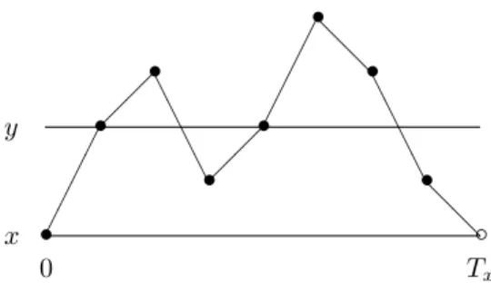
Why is (4.1) true? To go from i toj inm+n steps, we have to go from i to some state k in m steps and then from k to j in n steps.

The Markov property implies that the two parts of our journey are independent.

•

```````` aa

aa aa

aa

````````

i

j

time 0 m m+n

Proof of (4.1). We do this by combining the solutions of Q1 and Q2. Breaking things down according to the state at time m,

P(X_m+n=j|X₀ =i) =X

k

P(X_m+n =j, X_m =k|X₀ =i)

(19)

Using the definition of conditional probability as in the solution of Q1,

P(X_m+n=j, X_m =k|X₀ =i) = P(X_m+n =j, X_m =k, X₀ =i) P(X₀ =i)

= P(X_m+n =j, X_m =k, X₀ =i)

P(Xm =k, X0 =i) · P(X_m =k, X₀ =i) P(X0 =i)

=P(Xm+n=j|Xm =k, X0 =i)·P(Xm =k|X0 =i) By the Markov property (1.1) the last expression is

=P(Xm+n=j|Xm =k)·P(Xm =k|X0 =i) = p^m(i, k)pⁿ(k, j) and we have proved (4.1).

Having established (4.1), we now return to computations.

Example 1.11. Gambler’s ruin. Suppose for simplicity thatN = 4 in Example 1.1, so that the transition probability is

0 1 2 3 4

0 1.0 0 0 0 0 1 0.6 0 0.4 0 0 2 0 0.6 0 0.4 0 3 0 0 0.6 0 0.4 4 0 0 0 0 1.0 To compute p² one row at a time we note:

p²(0,0) = 1 and p²(4,4) = 1, since these are absorbing states.

p²(1,3) = (.4)² = 0.16, since the chain has to go up twice.

p²(1,1) = (.4)(.6) = 0.24. The chain must go from 1 to 2 to 1.

p²(1,0) = 0.6. To be at 0 at time 2, the first jump must be to 0.

Leaving the cases i= 2,3 to the reader, we have

p² =







1.0 0 0 0 0

.6 .24 0 .16 0 .36 0 .48 0 .16

0 .36 0 .24 .4

0 0 0 0 1







(20)

Using a calculator one can easily compute

p²⁰ =







1.0 0 0 0 0

.87655 .00032 0 .00022 .12291

.69186 0 .00065 0 .30749

.41842 .00049 0 .00032 .58437

0 0 0 0 1







0 and 4 are absorbing states. Here we see that the probability of avoing absorption for 20 steps is 0.00054 from state 3, 0.00065 from state 2, and 0.00081 from state 1. Later we will see that

n→∞lim pⁿ=







1.0 0 0 0 0

57/65 0 0 0 8/65 45/65 0 0 0 20/65 27/65 0 0 0 38/65

0 0 0 0 1







(21)

1.3 Classification of States

We begin with some important notation. We are often interested in the behavior of the chain for a fixed initial state, so we will introduce the shorthand

P_x(A) =P(A|X₀ =x)

Later we will have to consider expected values for this probability and we will denote them by E_x.

Let T_y = min{n ≥ 1 :X_n = y} be the time of the first return toy (i.e., being there at time 0 doesn’t count), and let

ρ_yy =P_y(T_y <∞)

be the probability X_n returns to y when it starts at y. Intuitively, the Markov property implies that the probability X_n will return at least twice to y is ρ²_yy, since after the first return, the chain is at y, and the Markov property implies that the probability of a second return following the first is again ρ_yy.

To show that the reasoning in the last paragraph is valid, we have to introduce a definition and state a theorem.

Definition 1.2. We say that T is a stopping time if the occur- rence (or nonoccurrence) of the event “we stop at timen,” {T =n}

can be determined by looking at the values of the process up to that time: X₀, . . . , X_n.

To see that T_y is a stopping time note that

{T_y =n}={X₁ 6=y, . . . , Xn−1 6=y, X_n=y}

and that the right-hand side can be determined from X₀, . . . , X_n. Since stopping at timen depends only on the values X₀, . . . , X_n, and in a Markov chain the distribution of the future only depends on the past through the current state, it should not be hard to believe that the Markov property holds at stopping times. This fact can be stated formally as:

Theorem 1.2. Strong Markov property. Suppose T is a stopping time. Given that T = n and X_T = y, any other information about X₀, . . . X_T is irrelevant for predicting the future, and X_T_+k, k ≥0 behaves like the Markov chain with initial state y.

(22)

Why is this true? To keep things as simple as possible we will show only that

P(X_T₊₁=z|X_T =y, T =n) =p(y, z)

LetV_nbe the set of vectors (x₀, . . . , x_n) so that ifX₀ =x₀, . . . , X_n= x_n, then T = n and X_T = y. Breaking things down according to the values of X₀, . . . , X_n gives

P(X_T₊₁ =z, X_T =y, T =n) = X

x∈Vn

P(X_n+1 =z, X_n=x_n, . . . , X₀ =x₀)

= X

x∈Vn

P(X_n+1 =z|X_n=x_n, . . . , X₀ =x₀)P(X_n=x_n, . . . , X₀ =x₀) where in the second step we have used the multiplication rule

P(A∩B) =P(B|A)P(A)

For any (x₀, . . . , x_n) ∈ A we have T = n and X_T = y so x_n = y.

Using the Markov property, (1.1), and recalling the definition of V_n shows the above

P(X_T₊₁ =z, T =n, X_T =y) =p(y, z)X

x∈Vn

P(X_n=x_n, . . . , X₀ =x₀)

=p(y, z)P(T =n, X_T =y)

Dividing both sides by P(T = n, X_T =y) gives the desired result.

Definition 1.3. Let T_y¹ =T_y and for k ≥2 let

T_y^k = min{n > T_y^k−1 :X_n =y} (1.3) be the time of the kth return to y.

The strong Markov property implies that the conditional probability we will return one more time given that we have returned k−1 times is ρ_yy. This and induction implies that

P_y(T_y^k<∞) =ρ^k_yy (1.4) At this point, there are two possibilities:

(i) ρ_yy < 1: The probability of returning k times is ρ^k_yy → 0 as k → ∞. Thus, eventually the Markov chain does not find its way

(23)

back to y. In this case the state y is called transient, since after some point it is never visited by the Markov chain.

(ii) ρ_yy = 1: The probability of returning k times ρⁿ_yy = 1, so the chain returns to y infinitely many times. In this case, the state y is called recurrent, it continually recurs in the Markov chain.

To understand these notions, we turn to our examples, beginning with

Example 1.12. Gambler’s ruin. Consider, for concreteness, the case N = 4.

0 1 2 3 4 0 1 0 0 0 0 1 .6 0 .4 0 0 2 0 .6 0 .4 0 3 0 0 .6 0 .4 4 0 0 0 0 1

We will show that eventually the chain gets stuck in either the bankrupt (0) or happy winner (4) state. In the terms of our re- cent definitions, we will show that states 0 < y < 4 are transient, while the states 0 and 4 are recurrent.

It is easy to check that 0 and 4 are recurrent. Since p(0,0) = 1, the chain comes back on the next step with probability one, i.e.,

P₀(T₀ = 1) = 1

and hence ρ₀₀ = 1. A similar argument shows that 4 is recurrent.

In general if y is an absorbing state, i.e., if p(y, y) = 1, then y is a very strongly recurrent state – the chain always stays there.

To check the transience of the interior states, 1,2,3, we note that starting from 1, if the chain goes to 0, it will never return to 1, so the probability of never returning to 1,

P₁(T₁ =∞)≥p(1,0) = 0.6>0

Similarly, starting from 2, the chain can go to 1 and then to 0, so P₂(T₂ =∞)≥p(2,1)p(1,0) = 0.36>0

Finally for starting from 3, we note that the chain can go immedi- ately to 4 and never return with probability 0.4, so

P₃(T₃ =∞)≥p(3,4) = 0.4>0

(24)

Generalizing from our experience with the gambler’s ruin chain, we come to a general result that will help us identify transient states.

Definition 1.4. We say that x communicates with y and write x→y if there is a positive probability of reaching ystarting from x, that is, the probability

ρ_xy =P_x(T_y <∞)>0

Note that the last probability includes not only the possibility of jumping from x to y in one step but also going from x to y after visiting several other states in between. The following property is simple but useful. Here and in what follows, lemmas are a means to prove the more important conclusions called theorems. To make it easier to locate things, theorems and lemmas are numbered in the same sequence.

Lemma 1.1. If x→y and y →z, then x→z.

Proof. Since x → y there is an m so that p^m(x, y) > 0. Similarly there is annso thatpⁿ(y, z)>0. Sincep^m+n(x, z)≥p^m(x, y)pⁿ(y, z) it follows that x→z.

Theorem 1.3. If ρ_xy >0, but ρ_yx <1, then x is transient.

Proof. Let K = min{k : p^k(x, y) > 0} be the smallest number of steps we can take to get from x toy. Sincep^K(x, y)>0 there must be a sequence y1, . . . yK−1 so that

p(x, y₁)p(y₁, y₂)· · ·p(yK−1, y)>0

SinceK is minimal all they_i 6=y(or there would be a shorter path), and we have

P_x(T_x =∞)≥p(x, y₁)p(y₁, y₂)· · ·p(y_K−1, y)(1−ρ_yx)>0 so x is transient.

We will see later that Theorem 1.3 allows us to to identify all the transient states when the state space is finite. An immediate consequence of Theorem 1.3 is

Lemma 1.2. If x is recurrent and ρ_xy >0 then ρ_yx= 1.

Proof. If ρ_yx<1 then Lemma 1.3 would imply x is transient.

(25)

In some cases it is easy to identify recurrent states.

Example 1.13. Social mobility. Recall that the transition probability is

1 2 3 1 .7 .2 .1 2 .3 .5 .2 3 .2 .4 .4

To begin we note that no matter whereX_n is, there is a probability of at least .1 of hitting 3 on the next step so P₃(T₃ > n) ≤ (.9)ⁿ. As n → ∞, (.9)ⁿ →0 so P3(T3 < ∞) = 1, i.e., we will return to 3 with probability 1. The last argument applies even more strongly to states 1 and 2, since the probability of jumping to them on the next step is always at least .2. Thus all three states are recurrent.

The last argument generalizes to the give the following useful fact.

Lemma 1.3. Suppose P_x(T_y ≤ k) ≥ α > 0 for all x in the state space S. Then

P_x(T_y > nk)≤(1−α)ⁿ

To be able to analyze any finite state Markov chain we need some theory. To motivate the developments consider

Example 1.14. A Seven-state chain. Consider the transition probability:

1 2 3 4 5 6 7 1 .3 0 0 0 .7 0 0 2 .1 .2 .3 .4 0 0 0 3 0 0 .5 .5 0 0 0 4 0 0 0 .5 0 .5 0 5 .6 0 0 0 .4 0 0 6 0 0 0 0 0 .2 .8 7 0 0 0 1 0 0 0

To identify the states that are recurrent and those that are transient, we begin by drawing a graph that will contain an arc from i toj if p(i, j)>0 and i6=j. We do not worry about drawing the self-loops corresponding to states withp(i, i)>0 since such transitions cannot help the chain get somewhere new.

(26)

In the case under consideration we draw arcs from 1→5, 2→1, 2→3, 2→4, 3→4, 4 →6, 4→7, 5→1, 6→4, 6→7, 7 →4.

5 3 7

1 2 4 6

? 6

- - 6

The state 2 communicates with 1, which does not communicate with it, so Theorem 1.3 implies that 2 is transient. Likewise 3 communicates with 4, which doesn’t communicate with it, so 3 is transient. To conclude that all the remaining states are recurrent we will introduce two definitions and a fact.

Definition 1.5. A set A isclosed if it is impossible to get out, i.e., if i∈A and j 6∈A then p(i, j) = 0.

In Example 1.14, {1,5} and {4,6,7} are closed sets. Their union, {1,4,5,6,7}is also closed. One can add 3 to get another closed set {1,3,4,5,6,7}. Finally, the whole state space {1,2,3,4,5,6,7} is always a closed set.

Among the closed sets in the last example, some are obviously too big. To rule them out, we need a definition.

Definition 1.6. A set B is calledirreducible if wheneveri, j ∈B, i communicates with j.

The irreducible closed sets in the Example 1.14 are{1,5}and{4,6,7}.

The next result explains our interest in irreducible closed sets.

Theorem 1.4. If C is a finite closed and irreducible set, then all states in C are recurrent.

Before entering into an explanation of this result, we note that The- orem 1.4 tells us that 1, 5, 4, 6, and 7 are recurrent, completing our study of the Example 1.14 with the results we had claimed earlier.

In fact, the combination of Theorem 1.3 and 1.4 is sufficient to classify the states in any finite state Markov chain. An algorithm will be explained in the proof of the following result.

(27)

Theorem 1.5. If the state space S is finite, then S can be written as a disjoint union T ∪R₁∪ · · · ∪R_k, where T is a set of transient states and the R_i, 1≤i≤k, are closed irreducible sets of recurrent states.

Proof. Let T be the set of x for which there is a y so that x → y buty 6→x. The states inT are transient by Theorem 1.3. Our next step is to show that all the remaining states, S−T, are recurrent.

Pick an x ∈ S −T and let C_x = {y : x → y}. Since x 6∈ T it has the property if x→ y, then y→ x. To check that Cx is closed note that if y ∈ Cx and y → z, then Lemma 1.1 implies x → z so z ∈C_x. To check irreducibility, note that if y, z ∈C_x, then by our first observationy→x and we havex→z by definition, so Lemma 1.1 implies y → z. C_x is closed and irreducible so all states in C_x are recurrent. LetR₁ =C_x. IfS−T −R₁ =∅, we are done. If not, pick a site w∈S−T −R₁ and repeat the procedure.

* * * * * * *

The rest of this section is devoted to the proof of Theorem 1.4.

To do this, it is enough to prove the following two results.

Lemma 1.4. If x is recurrent and x→y, then y is recurrent.

Lemma 1.5. In a finite closed set there has to be at least one recurrent state.

To prove these results we need to introduce a little more theory.

Recall the time of thekth visit to y defined by T_y^k = min{n > T_y^k−1 :X_n=y}

and ρ_xy =P_x(T_y <∞) the probability we ever visit y at some time n ≥1 when we start from x. Using the strong Markov property as in the proof of (1.4) gives

Px(T_y^k<∞) =ρxyρ^k−1_yy . (1.5) Let N(y) be the number of visits to y at times n ≥ 1. Using (1.5) we can compute EN(y).

Lemma 1.6. E_xN(y) = ρ_xy/(1−ρ_yy)

(28)

Proof. Accept for the moment the fact that for any nonnegative integer valued random variable X, the expected value of X can be computed by

EX =

∞

X

k=1

P(X ≥k) (1.6)

We will prove this after we complete the proof of Lemma 1.6. Now the probability of returning at least k times, {N(y) ≥ k}, is the same as the event that the kth return occurs, i.e., {T_y^k < ∞}, so using (1.5) we have

E_xN(y) =

∞

X

k=1

P(N(y)≥k) =ρ_xy

∞

X

k=1

ρ^k−1_yy = ρ_xy 1−ρyy

since P∞

n=0θⁿ= 1/(1−θ) whenever |θ|<1.

Proof of (1.6). Let 1_{X_≥k} denote the random variable that is 1 if X ≥k and 0 otherwise. It is easy to see that

X =

∞

X

k=1

1{X≥k}.

Taking expected values and noticing E1_{X≥k} =P(X ≥k) gives EX =

∞

X

k=1

P(X ≥k)

Our next step is to compute the expected number of returns to y in a different way.

Lemma 1.7. E_xN(y) =P∞

n=1pⁿ(x, y).

Proof. Let 1{X_n=y} denote the random variable that is 1 if X_n =y, 0 otherwise. Clearly

N(y) =

∞

X

n=1

1{Xn=y}. Taking expected values now gives

E_xN(y) =

∞

X

n=1

P_x(X_n =y)

(29)

With the two lemmas established we can now state our next main result.

Theorem 1.6. y is recurrent if and only if

∞

X

n=1

pⁿ(y, y) =E_yN(y) =∞

Proof. The first equality is Lemma 1.7. From Lemma 1.6 we see that EyN(y) = ∞ if and only if ρyy = 1, which is the definition of recurrence.

With this established we can easily complete the proofs of our two lemmas .

Proof of Lemma 1.4 . Suppose x is recurrent and ρ_xy > 0. By Lemma 1.2 we must have ρ_yx>0. Pickj and ` so thatp^j(y, x)>0 and p^`(x, y) > 0. p^j+k+`(y, y) is probability of going from y to y in j +k +` steps while the product p^j(y, x)p^k(x, x)p^`(x, y) is the probability of doing this and being at xat times j and j+k. Thus we must have

∞

X

k=0

p^j+k+`(y, y)≥p^j(y, x)

∞

X

k=0

p^k(x, x)

!

p^`(x, y) If x is recurrent then P

kp^k(x, x) = ∞, so P

mp^m(y, y) = ∞ and Theorem 1.6 implies that y is recurrent.

Proof of Lemma 1.5. If all the states inC are transient then Lemma 1.6 implies thatExN(y)<∞ for allxand yinC. SinceC is finite, using Lemma 1.7

∞>X

y∈C

E_xN(y) =X

y∈C

∞

X

n=1

pⁿ(x, y)

=

∞

X

n=1

X

y∈C

pⁿ(x, y) =

∞

X

n=1

1 =∞

where in the next to last equality we have used that C is closed.

This contradiction proves the desired result.

(30)

1.4 Stationary Distributions

In the next section we will show that if we impose an additional assumption called aperiodicity an irreducible finite state Markov chain converges to a stationary distribution

pⁿ(x, y)→π(y)

To prepare for that this section introduces stationary distributions and shows how to compute them. Our first step is to consider What happens in a Markov chain when the initial state is random? Breaking things down according to the value of the initial state and using the definition of conditional probability

P(X_n =j) =X

i

P(X₀ =i, X_n =j)

=X

i

P(X0 =i)P(Xn=j|X0 =i)

If we introduce q(i) = P(X₀ = i), then the last equation can be written as

P(X_n =j) =X

i

q(i)pⁿ(i, j) (1.7) In words, we multiply the transition matrix on the left by the vector q of initial probabilities. If there arek states, thenpⁿ(x, y) is ak×k matrix. So to make the matrix multiplication work out right, we should take q as a 1×k matrix or a “row vector.”

Example 1.15. Consider the weather chain (Example 1.3) and suppose that the initial distribution is q(1) = 0.3 and q(2) = 0.7. In this case

.3 .7

.6 .4 .2 .8

= .32 .68 since .3(.6) +.7(.2) = .32

.3(.4) +.7(.8) = .68

Example 1.16. Consider the social mobility chain (Example 1.4) and suppose that the initial distribution: q(1) =.5, q(2) = .2, and q(3) = .3. Multiplying the vector q by the transition probability

(31)

gives the vector of probabilities at time 1.

.5 .2 .3





.7 .2 .1 .3 .5 .2 .2 .4 .4



= .47 .32 .21

To check the arithmetic note that the three entries on the right-hand side are

.5(.7) +.2(.3) +.3(.2) =.35 +.06 +.06 = .47 .5(.2) +.2(.5) +.3(.4) =.10 +.10 +.12 = .32 .5(.1) +.2(.2) +.3(.4) =.05 +.04 +.12 = .21

If the distribution at time 0 is the same as the distribution at time 1, then by the Markov property it will be the distribution at all times n ≥1.

Definition 1.7. If qp=q then q is called a stationary distribution.

Stationary distributions have a special importance in the theory of Markov chains, so we will use a special letterπto denote solutions of the equation

πp=π.

To have a mental picture of what happens to the distribution of probability when one step of the Markov chain is taken, it is useful to think that we have q(i) pounds of sand at state i, with the total amount of sand P

iq(i) being one pound. When a step is taken in the Markov chain, a fraction p(i, j) of the sand at i is moved to j. The distribution of sand when this has been done is

qp=X

i

q(i)p(i, j)

If the distribution of sand is not changed by this procedure q is a stationary distribution.

Example 1.17. Weather chain. To compute the stationary distribution we want to solve

π₁ π₂

.6 .4 .2 .8

= π₁ π₂

(32)

Multiplying gives two equations:

.6π₁+.2π₂ =π₁ .4π1+.8π2 =π2

Both equations reduce to .4π1 =.2π2. Since we want π1+π2 = 1, we must have .4π₁ =.2−.2π₁, and hence

π₁ = .2

.2 +.4 = 1

3 π₂ = .4

.2 +.4 = 2 3 To check this we note that

1/3 2/3

.6 .4 .2 .8

= .6

3 +.4 3

.4 3 +1.6

3

General two state transition probability.

1 2

1 1−a a 2 b 1−b

We have written the chain in this way so the stationary distribution has a simple formula

π₁ = b

a+b π₂ = a

a+b (1.8)

As a first check on this formula we note that in the weather chain a = 0.4 and b = 0.2 which gives (1/3,2/3) as we found before. We can prove this works in general by drawing a picture:

•1 b

a+b •2 a

a+b

−→a

←−b

In words, the amount of sand that flows from 1 to 2 is the same as the amount that flows from 2 to 1 so the amount of sand at each site stays constant. To check algebraically that πp =π:

b

a+b(1−a) + a

a+bb = b−ba+ab

a+b = b

a+b b

a+ba+ a

a+b(1−b) = ba+a−ab

a+b = a

a+b (1.9) Formula (1.8) gives the stationary distribution for any two state chain, so we progress now to the three state case and consider the

(33)

Example 1.18. Social Mobility (continuation of 1.4).

1 2 3 1 .7 .2 .1 2 .3 .5 .2 3 .2 .4 .4 The equation πp=π says

π₁ π₂ π₃





.7 .2 .1 .3 .5 .2 .2 .4 .4



= π₁ π₂ π₃ which translates into three equations

.7π₁+.3π₂+.2π₃ = π₁ .2π₁+.5π₂+.4π₃ = π₂ .1π₁+.2π₂+.4π₃ = π₃

Note that the columns of the matrix give the numbers in the rows of the equations. The third equation is redundant since if we add up the three equations we get

π₁+π₂+π₃ =π₁+π₂+π₃

If we replace the third equation by π₁+π₂ +π₃ = 1 and subtract π₁ from each side of the first equation and π₂ from each side of the second equation we get

−.3π₁ +.3π₂+.2π₃ = 0 .2π₁−.5π₂+.4π₃ = 0

π₁+π₂ +π₃ = 1 (1.10) At this point we can solve the equations by hand or using a calculator.

By hand. We note that the third equation impliesπ₃ = 1−π₁− π₂ and substituting this in the first two gives

.2 = .5π1−.1π2

.4 = .2π₁+.9π₂

Multiplying the first equation by .9 and adding.1 times the second gives

2.2 = (0.45 + 0.02)π₁ or π₁ = 22/47

(34)

Multiplying the first equation by .2 and adding−.5 times the second gives

−0.16 = (−.02−0.45)π₂ or π₂ = 16/47 Since the three probabilities add up to 1, π3 = 9/47.

Using the TI83 calculator is easier. To begin we write (1.10) in matrix form as

π₁ π₂ π₃





−.2 .1 1 .2 −.4 1

.3 .3 1



= 0 0 1

If we let A be the 3×3 matrix in the middle this can be written as πA= (0,0,1). Multiplying on each side byA⁻¹ we see that

π = (0,0,1)A⁻¹

which is the third row ofA⁻¹. To computeA⁻¹, we enterAinto our calculator (using the MATRX menu and its EDIT submenu), use the MATRIX menu to put [A] on the computation line, press x⁻¹, and then ENTER. Reading the third row we find that the stationary distribution is

(0.468085, 0.340425, 0.191489)

Converting the answer to fractions using the first entry in the MATH menu gives

(22/47, 16/47, 9/47)

Example 1.19. Brand Preference (continuation of 1.5).

1 2 3 1 .8 .1 .1 2 .2 .6 .2 3 .3 .3 .4

Using the first two equations and the fact that the sum of theπ’s is 1

.8π₁+.2π₂+.3π₃ = π₁ .1π₁+.6π₂+.3π₃ = π₂ π₁+π₂+π₃ = 1

(35)

Subtracting π₁ from both sides of the first equation and π₂ from both sides of the second, this translates intoπA= (0,0,1) with

A=





−.2 .1 1 .2 −.4 1

.3 .3 1





Note that here and in the previous example the first two columns of A consist of the first two columns of the transition probability with 1 subtracted from the diagonal entries, and the final column is all 1’s. Computing the inverse and reading the last row gives

(0.545454, 0.272727, 0.181818)

Converting the answer to fractions using the first entry in the MATH menu gives

(6/11, 3/11, 2/11) To check this we note that

6/11 3/11 2/11





.8 .1 .1 .2 .6 .2 .3 .3 .4





=

4.8 +.6 +.6 11

.6 + 1.8 +.6 11

.6 +.6 +.8 11

Example 1.20. Basketball (continuation of 1.10). To find the stationary matrix in this case we can follow the same procedure. A consists of the first three columns of the transition matrix with 1 subtracted from the diagonal, and a final column of all 1’s.

−1/4 1/4 0 1

0 −1 2/3 1

2/3 1/3 −1 1

0 0 1/2 1

The answer is given by the fourth row of A⁻¹:

(0.5,0.1875, 0.1875, 0.125) = (1/2, 3/16, 3/16, 1/8) Thus the long run fraction of time the player hits a shot is

π(HH) +π(M H) = 0.6875 = 11/36.

(36)

1.5 Limit Behavior

Ifyis a transient state, thenP∞

n=1pⁿ(x, y)<∞for any initial state x and hence

pⁿ(x, y)→0

In view of the decomposition theorem, Theorem 1.5 we can now restrict our attention to chains that consist of a single irreducible class of recurrent states. Our first example shows one problem that can prevent the convergence of pⁿ(x, y).

Example 1.21. Ehrenfest chain (continuation of 1.2). For concreteness, suppose there are three balls. In this case the transition probability is

0 1 2 3

0 0 3/3 0 0

1 1/3 0 2/3 0 2 0 2/3 0 1/3

3 0 0 3/3 0

In the second power of p the zero pattern is shifted:

0 1 2 3

0 1/3 0 2/3 0 1 0 7/9 0 2/9 2 2/9 0 7/9 0 3 0 2/3 0 1/3

To see that the zeros will persist, note that if we have an odd number of balls in the left urn, then no matter whether we add or subtract one the result will be an even number. Likewise, if the number is even, then it will be odd on the next one step. This alternation between even and odd means that it is impossible to be back where we started after an odd number of steps. In symbols, if n is odd then pⁿ(x, x) = 0 for all x.

To see that the problem in the last example can occur for multi- ples of any number N consider:

Example 1.22. Renewal chain. We will explain the name later.

For the moment we will use it to illustrate “pathologies.” Let f_k be a distribution on the positive integers and let p(0, k−1) =f_k. For

(37)

states i >0 we let p(i, i−1) = 1. In words the chain jumps from 0 tok−1 with probability f_k and then walks back to 0 one step at a time. IfX₀ = 0 and the jump is tok−1 then it returns to 0 at time k. If say f₅ =f₁₅ = 1/2 then pⁿ(0,0) = 0 unless n is a multiple of 5.

Definition 1.8. The period of a state is the largest number that will divide all the n ≥ 1 for which pⁿ(x, x) > 0. That is, it is the greatest common divisor of I_x ={n ≥1 :pⁿ(x, x)>0}.

To check that this definition works correctly, we note that in Exam- ple 1.21, {n ≥ 1 : pⁿ(x, x) > 0} = {2,4, . . .}, so the greatest common divisor is 2. Similarly, in Example 1.22, {n ≥ 1 : pⁿ(x, x) >

0} ={5,10, . . .}, so the greatest common divisor is 5. As the next example shows, things aren’t always so simple.

Example 4.4. Triangle and square. Consider the transition matrix:

−2 −1 0 1 2 3

−2 0 0 1 0 0 0

−1 1 0 0 0 0 0 0 0 0.5 0 0.5 0 0

1 0 0 0 0 1 0

2 0 0 0 0 0 1

In words, from 0 we are equally likely to go to 1 or −1. From −1 we go with probability one to −2 and then back to 0, from 1 we go to 2 then to 3 and back to 0. The name refers to the fact that 0 → −1 → −2 → 0 is a triangle and 0 → 1 → 2 → 3 → 0 is a square.

-

?

? 6

-1 0 1

-2 3 2

1/2 1/2

•

Clearly, p³(0,0)>0 and p⁴(0,0)>0 so 3,4∈I₀. To compute I₀ the following is useful:

(38)

Lemma 1.8. I_x is closed under addition. That is, if i, j ∈I_x, then i+j ∈I_x.

Proof. If i, j ∈I_x then pⁱ(x, x)>0 and p^j(x, x)>0 so p^i+j(x, x)≥pⁱ(x, x)p^j(x, x)>0 and hence i+j ∈Ix.

Using this we see that

I0 ={3,4,6,7,8,9,10,11, . . .}

Note that in this example once we have three consecutive numbers (e.g., 6,7,8) inI₀ then 6 + 3,7 + 3,8 + 3∈I₀and hence it will contain all the larger integers.

For another unusual example consider the renewal chain (Exam- ple 1.22) with f₅ =f₁₂= 1/2. 5,12∈I₀ so using Lemma 1.8

I₀ ={5,10,12,15,17,20,22,24,25,27,29,30,32, 34,35,36,37,39,40,41,42,43, . . .}

To check this note that 5 gives rise to 10=5+5 and 17=5+12, 10 to 15 and 22, 12 to 17 and 24, etc. Once we have five consecutive numbers in I₀, here 39–43, we have all the rest. The last two examples motivate the following.

Lemma 1.9. If xhas period 1, i.e., the greatest common divisor I_x is 1, then there is a number n₀ so that if n ≥ n₀, then n ∈ I_x. In words, I_x contains all of the integers after some value n₀.

Proof. We begin by observing that it enough to show that Ix will contain two consecutive integers: kandk+1. For then it will contain 2k,2k+ 1,2k+ 2, or in general jk, jk+ 1, . . . jk+j. For j ≥k−1 these blocks overlap and no integers are left out. In the last example 24,25 ∈ I₀ implies 48,49,50 ∈ I₀ which implies 72,73,74,75 ∈ I₀ and 96,97,98,99,100∈I₀.

To show that there are two consecutive integers, we cheat and use a fact from number theory: if the greatest common divisor of a set I_x is 1 then there are integers i₁, . . . i_m ∈ I_x and (positive or negative) integer coefficients c_i so that c₁i₁+· · ·+c_mi_m = 1. Let a_i =c⁺_i andb_i = (−c_i)⁺. In words thea_i are the positive coefficients

(39)

and the b_i are −1 times the negative coefficients. Rearranging the last equation gives

a₁i₁+· · ·+a_mi_m = (b₁i₁+· · ·+b_mi_m) + 1

and using Lemma 1.8 we have found our two consecutive integers in I_x.

While periodicity is a theoretical possibility, it rarely manifests itself in applications, except occasionally as an odd-even parity problem, e.g., the Ehrenfest chain. In most cases we will find (or design) our chain to be aperiodic, i.e., all states have period 1. To be able to verify this property for examples, we need to discuss some theory.

Lemma 1.10. If p(x, x)>0, then x has period 1.

Proof. Ifp(x, x)>0, then 1∈I_x, so the greatest common divisor is 1.

This is enough to show that all states in the weather chain (Exam- ple 1.3), social mobility (Example 1.4), and brand preference chain (Example 1.5) are aperiodic. For states with zeros on the diagonal the next result is useful.

Lemma 1.11. If ρ_xy >0 and ρ_yx >0 then x and y have the same period.

Why is this true? The short answer is that if the two states have different periods, then by going fromxtoy, fromytoyin the various possible ways, and then from y to x, we will get a contradiction.

Proof. Suppose that the period of x is c, while the period of y is d < c. Let k be such that p^k(x, y) > 0 and let m be such that p^m(y, x)>0. Since

p^k+m(x, x)≥p^k(x, y)p^m(y, x)>0

we havek+m ∈Ix. Since xhas periodc, k+mmust be a multiple of c. Now let ` be any integer with p^`(y, y)>0. Since

p^k+`+m(x, x)≥p^k(x, y)p^`(y, y)p^m(y, x)>0

k+`+m ∈Ix, and k+`+m must be a multiple ofc. Sincek+m is itself a multiple of c, this means that ` is a multiple of c. Since

` ∈ I_y was arbitrary, we have shown that c is a divisor of every element ofI_y, butd < c is the greatest common divisor, so we have a contradiction.

(40)

Lemma 1.11 easily settles the question for the inventory chain (Example 1.6)

0 1 2 3 4 5 0 0 0 .1 .2 .4 .3 1 0 0 .1 .2 .4 .3 2 .3 .4 .3 0 0 0 3 .1 .2 .4 .3 0 0 4 0 .1 .2 .4 .3 0 5 0 0 .1 .2 .4 .3

Since p(x, x) > 0 for x = 2,3,4,5, Lemma 1.10 implies that these states are aperiodic. Since this chain is irreducible it follows from Lemma 1.11 that 0 and 1 are aperiodic.

Consider now the basketball chain (Example 1.10):

HH HM MH MM

HH 3/4 1/4 0 0

HM 0 0 2/3 1/3

MH 2/3 1/3 0 0

MM 0 0 1/2 1/2

Lemma 1.10 implies that HH and MM are aperiodic. Since this chain is irreducible it follows from Lemma 1.11 that HM and MH are aperiodic.

We now come to the main results of the chapter.

Theorem 1.7. Convergence theorem. Suppose p is irreducible, aperiodic, and has a stationary distribution π. Then as n → ∞, pⁿ(x, y)→π(y).

Corollary. If p is irreducible and has stationary distribution π, it is unique.

Proof. First suppose thatpis aperiodic. If there were two stationary distributions, π₁ and π₂, then by applying Theorem 1.7 we would conclude that

π₁(y) = lim

n→∞pⁿ(x, y) = π₂(y)

To get rid of the aperiodicity assumption, let I be the transition probability for the chain that never moves, i.e.,I(x, x) = 1 for allx, and define a new transition probability q= (I+p)/2, i.e., we either do nothing with probability 1/2 or take a step according to p. Since