A modi¯ed standard embedding with jumps in nonlinear optimization
¤JÄurgen Guddat
1)Francisco Guerra V¶azquez
2)Dieter Nowack
1)Jan-J. RÄuckmann
2)Abstract. The paper deals with a combination of pathfollowing methods (embedding approach) and feasible descent direction methods (so-called jumps) for solving a non- linear optimization problem with equality and inequality constraints. Since the method that we propose here uses jumps from one connected component to another one, more than one connected component of the solution set of the corresponding one-parametric problem can be followed numerically. It is assumed that the problem under consider- ation belongs to a generic subset which was introduced by Jongen, Jonker and Twilt.
There already exist methods of this type for which each starting point of a jump has to be an endpoint of a branch of local minimizers. In this paper the authors propose a new method by allowing a larger set of starting points for the jumps which can be constructed at bifurcation and turning points of the solution set. The topological prop- erties of those cases where the method is not successful are analyzed and the role of constraint quali¯cations in this context is discussed. Furthermore, this new method is applied to a so-called modi¯ed standard embedding which is a particular construction without equality constraints. Finally, an algorithmic version of this new method as well as computational results are presented.
Key words: Parametric programming, pathfollowing methods with jumps, genericity, Jongen-Jonker-Twilt regularity, modi¯ed standard embedding
AMS subject classi¯cation: 90C 31, 90C26, 90 C30, 65 K05, 49M37
¤)This work was partially supported by Deutsche Forschungsgemeinschaft (DFG) under grant Gu 304/14-1 and the Sistema Nacional de Investigadores (SNI, M¶exico)
1) Humboldt-UniversitÄat zu Berlin, Institut fÄur Mathematik, 10099 Berlin, Germany.
Emails: guddat@mathematik.hu-berlin.de, nowack@mathematik.hu-berlin.de
2) Universidad de las Am¶ericas, Escuela de Ciencias, Sta. Catarina M¶artir, Cholula, Puebla 72820, M¶exico. Emails: fguerra@mail.udlap.mx, rueckman@mail.udlap.mx
1
1 INTRODUCTION 2
1 Introduction
LetIRnbe then-dimensional space with the Euclidean normk¢kandCk(IRn;IR),k ¸1 the space of k-times continuously di®erentiable functions. In this paper we consider the nonlinear optimization problem
(P) min ff(x)jx2Mg (1.1)
where the nonempty feasible set is de¯ned by ¯nitely many equality and inequality constraints as
M =fx 2IRnjhi(x) = 0; i2I; gj(x)·0; j 2Jg
with I =f1;:::;mg, m < n,J =f1;:::;sg, and f;hi;gj 2C3(IRn; IR), i 2 I, j 2 J. Furthermore, we introduce the one-parametric nonlinear optimization problem
P(t) min ff(x; t)j x 2 M(t)g (1.2)
where t 2 IR is a real parameter,
M(t) =fx 2 IRn j hi(x; t) = 0; i 2 I; gj(x; t)·0; j 2 Jg
and f; hi; gj 2 C3(IRn£ IR; IR), i 2 I, j 2 J. For sake of simplicity we assume that all functions in (1.1) and (1.2) are three times continuously di®erentiable although some of the results given here also hold for a lower degree of di®erentiability.
The embedding approachis a well-known method for the calculation of a solution point (local minimizer, stationary point, generalized critical point, etc.) of (P); its basic idea is to construct an auxiliary problem P(t) which satis¯es at least the following three conditions:
(A1) A solution point x0 of P(0) is known.
(A2) The set of solution points of P(t) is nonempty for all t 2[0;1].
(A3) P(1) is similar (in a certain sense) or equivalent with (P).
Then, by using a so-called pathfollowing (or homotopy or continuation) method a solution pointx¤ of the original problem (P) can be obtained by following numerically a solution path connecting (x0;0) and (x¤;1), i.e. one has to ¯nd a discretization
0 =t0 < ¢ ¢ ¢ < ti < ¢ ¢ ¢ < tN = 1
of the interval [0;1] and corresponding solution points x(ti) of P(ti), i= 0; : : : ; N (cf.
e.g. [1, 2, 3, 4, 5, 7, 8, 10, 12, 16, 18, 19, 21, 23]).
Example 1.1
As an example we present the so-called standard embedding which is de¯ned by the one-parametric problemPx0(t) min ftf(x) + (1¡ t)kx ¡ x0k2 j x 2 Mx0(t)g
1 INTRODUCTION 3 with the starting point x0 2 IRn and the feasible set
Mx0(t) =
(
x 2 IRn¯¯¯¯¯ hi(x) + (t ¡ 1)hi(x0) = 0; i 2 I
gj(x) + (t ¡1)gj(x0)·0; j 2 J
)
:
Obviously, (A1) and (A3) are satis¯ed but (A2) cannot be guaranteed in general (cf.
Example 5.1). In particular, the feasible set could be empty for some parameter values
t 2 (0;1).
However, in general, the existence of a solution curve to be followed is a very strong condition. In [16, 18], topological conditions are discussed which ensure an appropriate structure of the solution set of P(t) (union of one-dimensional manifolds) for the use of pathfollowing methods. In particular, Jongen, Jonker and Twilt de¯ned in [16] a particular open and dense subset F ½ C3(IRn £ IR; IR)1+m+s and described the corre- sponding topological structure of the solution set §gc of P(t) by de¯ning ¯ve di®erent types (the set of nondegenerate points and the singularities which may appear) such that §gc can be divided in ¯ve disjoint subsets.
Assuming that the function vector (f; hi; gj; i 2 I; j 2 J) in (1.2) belongs to this generic class F, Guddat, Guerra V¶azquez and Jongen presented in [12] some solution methods forP(t) which combine pathfollowing methods with so-called \jumps", where a \jump" refers to an appropriate feasible descent direction method (or, more general, NLP-solver) with the objective to calculate a solution point which belongs to another connected component of §gc (\jump from one connected component of §gc to another one"). Then, more than one connected component of §gc can be followed numerically and, hence, there are more chances to attain the parameter value t = 1 (note that standard pathfollowing methods are restricted to one connected component only). In [12], the jumps are de¯ned for points (starting points for the feasible descent direction method) which are end points of branches of local minimizers. By applying theoretical results from [14], in this paper we generalize the mentioned approach from [12] and in- troduce the method JUMP II¤ that combines pathfollowing methods with jumps which are de¯ned for a larger class of starting points. By means of this new method (per- haps) more connected components of §gc can be detected and numerically described.
Besides the goal of attaining the parameter value t= 1 (in the context of the embed- ding approach) another motivation for combining pathfollowing methods with jumps is the solution of optimization problems that depend naturally on a parameter; here, one is often interested in following more than one (or as many as possible) connected components of the solution set.
The goal of this paper is twofold:
Firstly, we discuss a particular one-parametric problemPm(t) which is calledmodi¯ed standard embedding; its construction yields that the feasible set is nonempty for all
t 2[0;1] (which is a necessary condition for (A2) and that, in general, is not satis¯ed for the standard embedding given in Example 1.1). Furthermore, an important feature for the use of feasible descent direction methods is thatP m(t) only has inequality con- straints although the original problem (P) may also have equality constraints.
2 NOTATIONS AND THEORETICAL BACKGROUND 4 Secondly, we introduce the method JUMP II¤ which combines pathfollowing methods with feasible descent direction methods (\jumps") where these jumps are de¯ned for a larger class of starting points (not only for those which are end points of a branch of local minimizers). The goal of JUMP II¤ is to follow as many connected components of
§gc (restricted to a given parameter interval) as possible. We analyze the topological situations for which we cannot attain the parameter value t = 1 and discuss the role of constraint quali¯cations in this context.
The paper is organized as follows. Section 2 contains basic results and we recall the generic class F which was introduced by Jongen, Jonker and Twilt (cf. [16]). In Sec- tion 3 we de¯ne the modi¯ed standard embedding and discuss its properties. Section 4 deals with the method JUMP II¤ which combines pathfollowing methods with jumps which are de¯ned for solution points of Types 1-4. Each possible situation for a jump is characterized and an algorithmic version of JUMP II¤ is presented. Finally, Section 5 contains computational results which illustrate the application of JUMP II¤ to the modi¯ed standard embedding. These numerical tests have been realized by means of the program package PAFO [9].
2 Notations and theoretical background
In this section we present some notations, basic results and we recall the open and dense class F of functions which was introduced by Jongen, Jonker and Twilt [16].
Critical point sets
Throughout the paper the problems (P) and P(t) are de¯ned as in (1.1) and (1.2), respectively. For ¹x 2 M(¹t) we denote the index set of active inequality constraints by
J0(¹x; ¹t) = fj 2 J j gj(¹x; ¹t) = 0g:
A point (¹x; ¹t) 2 IRn £ IR is called a generalized critical point (gc point) of P(¹t) (cf.
[12, 16]) if ¹x 2 M(¹t) and the gradients Dxf(¹x; ¹t), Dxhi(¹x; ¹t), i 2 I, Dxgj(¹x; ¹t), j 2 J0(¹x; ¹t) are linearly dependent. Obviously, if ¹x is a stationary point (for a de¯nition, see [12, p.1]) or a local minimizer of P(¹t), then (¹x;¹t) is also a gc point of P(¹t). We introduce the following sets for the problems (P) and P(t):
ªgc(P(t)) =f(x; t)2 IRn£ IR j(x; t) is a gc point of P(t)g;
ªstat(P(t)) = fx 2 IRn j x is a stationary point ofP(t)g;
ªloc(P(t)) = fx 2 IRn j xis a local minimizer of P(t)g;
ªglob(P(t)) =fx 2 IRn j x is a global minimizer of P(t)g;
ªstat(P) =fx 2 IRn j xis a stationary point of (P)g;
ªloc(P) =fx 2 IRnj is a local minimizer of (P)g:
Furthermore, de¯ne the unfolded sets
§gc =f(x; t)2 IRn£ IR j(x; t)2ªgc(P(t))g;
§stat =f(x; t)2 IRn£ IR j x 2 ªstat(P(t))g;
§loc =f(x; t)2 IRn£ IR j x 2ªloc(P(t))g:
2 NOTATIONS AND THEORETICAL BACKGROUND 5 Constraint quali¯cations
We will use the subsequent well-known constraint quali¯cations LICQ and MFCQ.
The Linear Independence constraint quali¯cation (brie°y, LICQ) is said to hold at
¹x 2 M(¹t) if the gradients Dxhi(¹x; ¹t), i 2 I, Dxgj(¹x; ¹t), j 2 J0(¹x; ¹t) are linearly inde- pendent.
TheMangasarian-Fromovitz constraint quali¯cation(brie°y,MFCQ) holds at ¹x 2 M(¹t) if
(MF 1) the gradients Dxhi(¹x; ¹t), i 2 I are linearly independent, (MF 2) there exists a vector » 2 Rn such that
Dxhi(¹x; ¹t)» = 0; i 2 I;
Dxgj(¹x; ¹t)» < 0; j 2 J0(¹x; ¹t):
Obviously (cf. e.g. [20]), if ¹x 2 ªloc(P(¹t)) and MFCQ or LICQ holds at ¹x 2 M(¹t), then ¹x 2 ªstat(P(¹t)).
The generic class F of Jongen, Jonker and Twilt
In the sequel we consider the function vector (f; H; G) 2 C3(IRn£ IR)1+m+s which characterizes the one-parametric problemP(t), whereH(x; t) = (h1(x; t); : : : ; hm(x; t)) and G(x; t) = (g1(x; t); : : : ; gs(x; t)).
It is well-known that the use of pathfollowing methods for the calculation of gc points (or stationary points or local minimizers) of P(t) requires a particular structure of the corresponding set §gc (or §stat or §loc). In [16], Jongen, Jonker and Twilt introduced an open and dense subset F of C3(IRn £ IR; IR)1+m+s which can be described by the topological structure of the corresponding set §gc for any (f; H; G)2 F. In particular, (f; H; G) 2 F implies that §gc consists locally of a ¯nite union of one-dimensional manifolds and, therefore, it has an appropriate structure for the use of pathfollowing methods. Below we cite our very short characterization from [12] of the class F; the complete description can be found in [16] (see [10] as well).
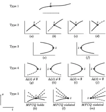
If (f; H; G)2 F, then §gc can be divided into ¯ve types of gc points:
Type 1: A point ¹z = (¹x; ¹t) 2 §gc is of Type 1 (non-degenerate gc point) if the following conditions are satis¯ed:
There exist ¹¸i; ¹¹j 2 IR, i 2 I, j 2 J0(¹z) with
³Dxf +X
i2I
¹¸iDxhi+ X
j2J0(¹z)
¹¹jDxgj
´jz=¹z= 0; (2.1)
LICQ is satis¯ed at ¹x 2 M(¹t); (2.2a)
(therefore ¹¸i, ¹¹j, i 2 I, j 2 J0(¹z) are uniquely de¯ned)
¹¹j 6= 0; j 2 J0(¹z); (2.2b)
D2xL(¹z)jT (¹z) is nonsingular; (2.2c)
2 NOTATIONS AND THEORETICAL BACKGROUND 6 where Dx2L is the Hessian of the Lagrangian
L(z) = f(z) +X
i2I
¹¸ihi(z) + X
j2J0(¹z)¹¹jgj(z);
and the uniquely determined numbers ¹¸i;¹¹j are taken from (2.1). Furthermore,
T(z) =f» 2 IRnj Dxhi(z)»= 0; i 2 I; Dxgj(z)» = 0; j 2 J0(z)g
is the tangent space atz. Dx2L(z)jT (z)representsVTDx2LV, where V is a matrix whose columns form a basis ofT(z). The nondegeneracy of a point of Type 1 implies that the subset of §gc which consists of all points of Type 1 forms a one-dimensional manifold.
The points of the Types 2-5 represent four basic degeneracies (see [16] for more details):
Type 2 { violation of (2.2b) Type 3 { violation of (2.2c)
Type 4 { violation of (2.2a) and jIj + jJ0(¹z)j < n + 1 Type 5 { violation of (2.2a) and jIj + jJ0(¹z)j = n + 1.
Figure 2.1 illustrates for each of the ¯ve types the local structure of §gc in a neigh- bourhood of a stationary point ¹z: the full curve stands for the set §stat and the dotted curve represents the set of gc points which are not stationary points.
Figure 2.1: The structure of §gc in a neighbourhood of ¹z 2 §stat.
2 NOTATIONS AND THEORETICAL BACKGROUND 7
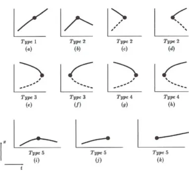
Figure 2.2: The structure of §stat in a neighbourhood of a local minimizer.
Figure 2.2 illustrates for each of the ¯ve types the local structure of §stat in a neigh- bourhood of a local minimizer: the full curve stands for the set §loc and the dotted curve in (c), (d), (e), (f) represents stationary points which are not local minimizers.
The dotted curve in (g), (h) represents stationary points (which are not local minimiz- ers) when J0(¹x) =;.
The points of the Types 2-5 constitute a discrete subset of §gc; in particular, the whole set §gc is the closure of the set of all points of Type 1. Therefore, (f; H; G)2 F implies an appropriate structure of §gc for the application of path-following methods.
Let §vgc be that subset of §gc which consists of all points of Typev, v= 1; : : : ;5. Then, we de¯ne the class F as
F =f(f; H; G)2 C3(IRn £ IR; IR)1+m+s j§gc= [5
v=1§vgcg:
For further analysis we need the following de¯nition:
De¯nition 2.1LetK ½ IRbe an interval. The one-parametric problemP(t) is called
regular in the sense of Jongen, Jonker and Twilt (brie°y, JJT-regular) with respect to K if
(IRn£ K)\§gc= (IRn£ K)\ [5
v=1§vgc:
The following two theorems give insight about the assumption that (f; H; G)2 F. The
¯rst one states a generic property that we already mentioned above.
2 NOTATIONS AND THEORETICAL BACKGROUND 8
Theorem 2.1
(Genericity theorem, cf. [16]). The class F is Cs -open and C3 s -dense3 in C3(IRn £ IR; IR)1+m+s, where Cs denotes the strong (or Whitney-) C3 s -topology3 (cf.[15, 17]).
The next theorem provides a special perturbation of (f; H; G) with additional parame- ters that can be chosen arbitrarily small and such that the perturbed functions belong to the class F. Let the space of symmetric n £ n-matrices be identi¯ed byIRn(n+1)=2.
Theorem 2.2
(Pertubation theorem, cf. [22]). Let (f; H; G)2 C3(IRn £ R; R)1+m+s.Then, for almost all
(b; A; c; D; e; F)2 IRn£ IRn(n+1)=2£ IRm £ IRmn £ IRs £ IRsn, we have (f(x; t) +bT x+xT Ax; H(x; t) +c+Dx; G(x; t) +e+F x)2 F:
Here \almost all" means: each measurable subset of
f(b; A; c; D; e; F)j(f(x; t) +bT x+xT Ax; H(x; t) +c+Dx; G(x; t) +e+Fx) =2 Fg has the Lebesgue-measure zero.
Exemplarily, the following theorem presents some conditions which imply the existence of a curve in §stat connecting a (known) stationary pointx0 ofP(0) with a (unknown) stationary point x¤ of P(1).
Theorem 2.3
(cf. [7]). Assume that(C1) M(t) is non-empty and there exists a compact set containing M(t) for all t 2 [0;1].
(C2) P(t) is JJT-regular with respect to [0;1].
(C3) There exists a t1 >0 and a continuous function x: [0; t1) ! IRn such that x(t) is the unique stationary point for P(t) for t 2 [0; t1).
(C4) MFCQ holds at all x 2 M(t) for all t 2 [0;1].
Then there exists a piecewise C3-path (brie°y, PC3-path) in §stat that connects (x0;0) (with x(0) =x0) with some point (x¤;1).
For a discussion of the assumptions of the latter theorem we refer to [7]. However, it can easily be seen from the topological properties of §gc that the condition (C4) is generically not ful¯lled, i.e. in general it cannot be satis¯ed by appropriate arbitrarily small perturbations of the function vector (f; H; G). We will return to this point later in the discussion of the heuristic method JUMP II¤ in Section 4, Remark 4.5.
3 A MODIFIED STANDARD EMBEDDING 9
3 A modi¯ed standard embedding
In order to ensure the existence of a curve in §gc connecting a gc point ofP(0) with a gc point of P(1) one has to assume that
M(t)6=;for all t 2[0;1]: (3.1)
In general, this assumption (3.1) is not ful¯lled for the standard embedding presented in Example 1.1 (see [6] for a corresponding example which will be considered again in Example 5.1). In this section we introduce the so-called modi¯ed standard embedding which satis¯es (3.1). The modi¯ed standard embedding Pm(t) for the problem (P) in (1.1) is de¯ned as follows (with q 2IR, q >0 and x0 2IRn):
Pm(t) min ff(x;t)j x2Mm(t)g; t2IR; (3.2) where
f(x;t) =tf(x) + (1¡t)kx¡x0k2;
Mm(t) =fx2IRnj gj(x;t)·0; j = 1;:::;m+s+ 2g; gi(x;t) =thi(x) +t¡1; i 2 I;
gm+j(x; t) = tgj(x) +t ¡1; j 2 J;
gm+s+1(x; t) =kxk2¡ q;
gm+s+2(x; t) =¡tX
i2I hi(x) +t ¡1:
Remark 3.1
Several modi¯cations of the standard embedding have been discussed in [6]. In (3.2), the additional \compacti¯cation constraint" gm+s+1 implies that M(t) is compact for all t 2 [0;1]; its consequences for the similarity of Pm(1) and (P) (cf.(A3)) are discussed in the subsequent Proposition 3.2. Furthermore, the fact that
Pm(t) does not have any equality constraint allows the application of corresponding descent methods for the realization of the so-called jumps (see Section 4). Note that the starting point x0 can be chosen arbitrarily.
In the next two propositions we will summarize several properties of the modi¯ed stan- dard embedding (cf. [6] for a more general discussion).
Proposition 3.1
Let q > 0inPm(t)be chosen such thatM \fx 2 IRn j kxk2 · qg 6= ;and kx0k2 < q. Then we have:
(i) Mm(t) is nonempty and compact for all t 2 [0; 1]. In particular,
Mm(1) = M \ fx 2 IRnj kxk2 · qg.
(ii) Mm(t2) ½ Mm(t1) for all t1 < t2; t1; t2 2 [0; 1]. (iii) ªglob(Pm(0)) = ªstat(Pm(0)) = fx0g.
(iv) ªglob(Pm(t)) is nonempty for all t 2 [0; 1].
(v) If I 6= ;, then the MFCQ does not hold at any point x 2 Mm(1).
3 A MODIFIED STANDARD EMBEDDING 10
(vi) If I 6=;, then Mm(t) =; for all t >1.
Proof. From the de¯nition of P m(t) we obtain easily (i)¡(iv). Now, letI 6=;. Then we have for x 2 Mm(1):
gi(x;1) =hi(x) = 0; i 2 I and gm+s+2(x;1) =¡X
i2I hi(x) = 0:
Obviously, there does not exist a vector » 2 IRn satisfying (MF2) and we obtain (v).
For the proof of (vi) assume that there exist ¹t > 1 and ¹x 2 Mm(¹t). Then, we obtain the contradiction
hi(¹x)· 1¡¹t
¹t <0; i 2 I and ¡X
i2I hi(¹x)· 1¡¹t
¹t : 4
The next proposition discusses properties of P m(0) as well as the similarity of the problems Pm(1) and (P). We omitted the proof because it is obvious.
Proposition 3.2 The following statements are true:
(i) If 0< kx0k2 < q, then each gc point of Pm(0) is non-degenerate (cf. the de¯nition of a gc point of Type 1 in Section 2).
(ii) If kxk¹ 2 < q and x 2¹ ªstat(Pm(1)) (resp. x 2¹ ªloc(P m(1))), then x 2¹ ªstat(P)
(resp. x 2¹ ªstat(P)).
(iii) ªgc(P m(1)) =Mm(1)£ f1g and Mm(1) =M \ fx 2 IRn j kxk2 · qg.
(iv) Let x 2¹ ªloc(P) and kxk¹ 2 · q. Then, x 2¹ ªloc(Pm(1)).
(v) Let x 2¹ ªstat(P) and kxk¹ 2 · q. Then, (¹x;1)2ªgc(Pm(1)).
(vi) If M µ fx 2 IRn j kxk2 · qg, then Pm(1) and (P) are equivalent, i.e. f(x;1) =
f(x) and Mm(1) =M. 4
Note that, by Proposition 3.1 (iii) and Proposition 3.2 (i), the starting point (x0;0) is a non-degenerate gc point and x0 a global minimizer of P m(0). Now, assume for a moment that each gc point of Mm(1) is of one of the ¯ve types of Jongen, Jonker and Twilt (i.e. it belongs to S5v=1§vgc, cf. Section 2). Then, by Proposition 3.2 (iii) and Proposition 3.1 (v), we have that ªgc(P m(1)) =Mm(1)£f1gand MFCQ does not hold at each ¹x 2 Mm(1) (i.e. (¹x;1) is not a point of Type 1) and, therefore,Mm(1) has to be a discrete subset (the points of the Types 2-5 constitute a discrete subset, cf. Section 2).
Since, in general, Mm(1) is not a discrete subset it makes no sense to assume that the problem Pm(t) is JJT-regular with respect to an interval K that contains the parameter value t = 1 (which would imply that each gc point of P m(1) belongs to
S5
v=1§vgc). Having that in mind we modify the Theorem 2.3 as follows.
3 A MODIFIED STANDARD EMBEDDING 11 Corollary 3.1 Assume that
(C2¤) Pm(t)is JJT-regular with respect to [0; 1).
(C4¤) MFCQ holds at all x 2 Mm(t) for all t 2 [0; 1).
Then, there exists for each ^t 2 (0;1) a PC3-path in §stat that connects (x0;0) with some point (^x;^t).
Proof. It follows directly from Theorem 2.3 and Proposition 3.1 (i), (iii). 4
Under the assumptions of Corollary 3.1 a sequence (xi; ti) 2 §stat with ti ! 1 can be created whose limit points are gc points of Pm(1) (since the set §gc is closed).
As already mentioned at the end of Section 2, the assumption (C4) of Theorem 2.3 - and, now, the assumption (C4¤) of Corollary 3.1 as well - are very strong conditions in the sense that they cannot be satis¯ed by perturbing (arbitrarily small) the function vector (f; H; G) (cf. Remark 4.5). However, next we present a condition on the con- straints hi(x),gj(x),i 2 I,j 2 J of (P) (which do not depend on the parametert) that ensures (C4¤). This kind of condition was discussed in [7, 13]; in [13], in the frame- work of penalty, exact penalty and Lagrange multiplier methods, it was introduced as Enlarged Mangasarian Fromovitz constraint quali¯cation (brie°y, EnMFCQ). We de-
¯ne the following modi¯cation of EnMFCQ, whereBq =fx 2 IRn j kxk2 · qgforq >0.
De¯nition 3.1 The Modi¯ed EnMFCQ is said to hold at Bq if for each x 2 Bq
there exists a vector » 2 IR such that:
hi(x) + Dhi(x)» · 0; i 2 fi 2 Ijhi(x) > 0g;
gj(x) + Dgj(x)» · 0; j 2 fj 2 Jjgj(x) > 0g;
2xT» < 0 if kxk2 = q;
¡X
i2I hi(x) ¡
ÃX
i2I Dhi(x)
!
» · 0 if X
i2Ihi(x) < 0:
Corollary 3.2 Assume that the Modi¯ed EnMFCQ holds at Bq. Then, the condition (C4¤) is ful¯lled.
Proof. First, let t = 0, ¹x 2 Mm(0) and kxk2 = q. Then, by the Modi¯ed EnMFCQ, we have 2¹x>» < 0 and we are done. Now, let ¹t 2 (0;1), ¹x 2 Mm(¹t) and consider any active constraint of (¹x;¹t), e.g.
¹thi(¹x) + ¹t ¡1 = 0 for some i 2 I:
Then, ¹thi(¹x) = 1¡¹t >0 and, by the Modi¯ed EnMFCQ, we have ¹thi(¹x)+¹tDhi(¹x)» ·0 and, hence, ¹tDhi(¹x)» <0. Since the active constraint was chosen arbitrarily, the proof
is complete. 4
Next we present a \justi¯cation theorem" for the assumption (C2¤) in Corollary 3.1
4 THE HEURISTIC METHOD JUMP II¤ 12 which is an application of Theorem 2.2. In particular, the perturbations used in the following Theorem 3.1 are related to the function vector (f;hi(x);gj(x);i2 I;j 2 J) which describes the original problem (P) (and which does not depend on t). Let the parameter vector (b;A;c;D)2 IRn £IRn(n+1)=2£IRm+s+1£IR(m+s+1)n with D = (d1;:::;dm+s+1),di 2IRn,i= 1:::;m+s+ 1 be given and \almost all" be de¯ned in an analogous way as in Theorem 2.2.
Theorem 3.1
For almost all (b; A; c; D) the modi¯ed standard embedding with the perturbed function vectortf(x) + (1¡ t)kx ¡ x0k2+ (1¡ t)(b>x+x>Ax)
thi(x) +t ¡1 + (1¡ t)(ci + (di)>x); i 2 I
tgj(x) +t ¡1 + (1¡ t)(cm+j+ (dm+j)>x); j 2 J
kxk2¡ q
¡tX
i2I hi(x) +t ¡1 + (1¡ t)(cm+s+1+ (dm+s+1)>x) is JJT-regular with respect to (¡1;1).
The proof is left to the reader because it applies straightforwardly the technique used in the proof of Theorem 2.2 (cf. [22]).
In the subsequent section we will describe a pathfollowing method with jumps where the problem under consideration is assumed to be JJT-regular. However, the strong condition (C4¤) need not be ful¯lled and we will see that the failure of (C4¤) may im- ply the method to stop at some parameter value t¤ <1, i.e. a gc point of the original problem (P) is not attained. In that sense the method to be presented is a heuristic one.
4 The heuristic method JUMP II
¤Throughout this section we refer to the one-parametric problem P(t) given in (1.2).
We present the heuristic method JUMP II¤ in a general form for the class of problems
P(t). Then, in Section 5, we will apply numerically JUMP II¤ to problems of the form P m(t) (cf. (3.2)) in order to obtain a gc point (or a stationary point or a local minimizer) of a given problem (P).
In [12], a pathfollowing method for the set §gc (called PATH III, cf. [12, Section 4.5]) is described which can be combined with so-called jumps (the corresponding methods are called JUMP I cf. [12, Section 5.2] and JUMP II cf. [12, Section 5.3]). A jump refers to an appropriate feasible descent direction method (or, more general, NLP- solver) applied to a starting point (x1; t1) 2 §gc with the objective to obtain a point (x2; t1)2§gc that belongs to another connected component of §gc than (x1; t1) (\jump from one connected component of §gc to another one"). Next we explain very brie°y the main ideas of PATH III and JUMP II; for more details we refer to [12].
4 THE HEURISTIC METHOD JUMP II¤ 13
PATH III
The method computes, for a given interval [tA; tB] ½ IR, tA < 0 < tB, a numeri- cal description of a compact connected component of §gc \(IRn£[tA; tB]) assuming that P(t) is JJT-regular with respect to [tA; tB]. In particular, PATH III ¯nds a dis- cretization of [tA; tB] and corresponding gc points starting at (x0;0)2§gc (cf. (A1) in Section 1). The method is based on an active-index-set strategy and uses a so-called predictor-corrector scheme for those parts with constant active index sets. A Newton- like corrector is applied which implies a superlinear rate of convergence. We mention two important features of this approach: the computation of the new index sets for all possible continuations at points of Types 2 and 5 (cf. Figure 2.1) as well as the pathfollowing of the turning points of Types 3 and 4 (cf. Figure 2.1).
Remark 4.1
If [0;1] ½ [tA; tB] and if there exists a PC3-path in §stat connecting (x0;0) and (x¤;1) (cf. Theorem 2.3), then PATH III also refers to the standard proce- dure of the embedding approach: A ¯nite discretization0 =t0 < t1 < ¢ ¢ ¢ < ti < ¢ ¢ ¢ < tN = 1
of the interval [0;1] and corresponding approximations ~x(ti) of stationary points x(ti) of P(ti) are obtained.
JUMP II
The goal of JUMP II is to ¯nd a numerical description of ¯nitely many connected components of §gc\(IRn£[tA; tB]) by combining PATH III (for the numerical descrip- tion of each connected component) with jumps in §gc. The jumps (feasible descent direction method, NLP-solver) are de¯ned for gc points of Type 1 and for gc points fromcl§loc (wherecldenotes the closure) which are of Type 2, 3 or 4. For more details on JUMP II we refer to the Examples 5.3.1, 5.3.2 and 5.3.3 as well as to the Figures 5.17, 5.18 and 5.19 in [12, Section 5.3].
Now we introduce the heuristic method JUMP II¤ as a generalization of JUMP II.
We refer to the forthcoming Remark 4.4 after the presentation of JUMP II¤ where some di®erences between JUMP II and JUMP II¤ are discussed.
JUMP II ¤
As for JUMP II, the goal of JUMP II¤ is to ¯nd a numerical description of ¯nitely many connected components of §gc\(IRn£[tA; tB]). However, in JUMP II¤ there exist more possibilities for \jumping from one connected component of §gc\(IRn£[tA; tB]) to another one" than in JUMP II.
Let [tA; tB]½ IRwith tA <0< tB and assume the following conditions:
(B1) P(t) is JJT-regular with respect to [tA; tB].
4 THE HEURISTIC METHOD JUMP II¤ 14 (B2) (x0;0)2§1gc is known.
(B3) M(t) is nonempty and there exists a compact set containing M(t) for all t 2 [tA; tB].
By using PATH III with the starting point (x0;0)2§1gc (cf. (B2)) assume that a con- nected component C of §gc\(IRn£[tA; tB]) with (x0;0)2 C is described numerically:
we have a (su±ciently ¯ne) discretization of the interval [tA; tB]:
tA · t¡q1 < ¢ ¢ ¢ < t0 = 0< ¢ ¢ ¢ < ti < ti+1< ¢ ¢ ¢ < tr1 · tB
as well as the corresponding sets C(ti) ½ §gc where C(ti) = f(x; t) 2 C j t = tig,
i 2 S =f¡q1; : : : ;0; : : : r1g with
C \
à 5 [
v=2§vgc
!
½ [
i2S
C(ti): (4.1)
The latter situation is depicted in [12, Figure 5.16]. By (B3) and since the gc points of Types 2-5 form a discrete set, the sets C \§vgc, v = 2; : : : ;5 are ¯nite and, hence, the condition (4.1) can be ful¯lled by a suitable choice of the step length in PATH III.
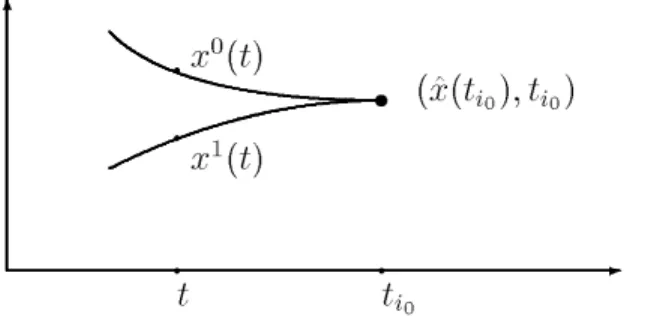
We calculate for each ti, i 2 S the points (^x(ti); ti)2 C and (¹x(ti); ti)2 C satisfying
f(^x(ti); ti)· f(x; ti) for all (x; ti)2 C(ti) (4.2) and
f(¹x(ti); ti)¸ f(x; ti) for all (x; ti)2 C(ti): (4.3) Note that ^x(ti) and ¹x(ti) need not be unique.
JUMP II¤ deals with the following 6 situations where for each of them a corresponding feasible descent direction exists: by applying a feasible descent direction method one obtains a gc point which does not belong to C (\jump from C to another connected component of §gc\(IRn£[tA; tB])") which will be described numerically by applying PATH III again). The Situations 1, 2 and 5 are cited from [12, Section 5.3] since they also appear in JUMP II. The proof and theoretical background for the descent direc- tions given in Situations 3, 4 and 6 can be found in [14].
Situation 1: There exists an i0 2 S with (^x(ti0); ti0)2 §1gcn§stat.
Then we obtain a feasible ¯rst order descent direction » 2 IRn by solving the system
Dxf(^x(ti0); ti0)» <0; Dxhi(^x(ti0); ti0)»= 0; i 2 I
Dxgj(^x(ti0); ti0)» ·0; j 2 J0(^x(ti0); ti0):
Situation 2: There exists an i0 2 S with (^x(ti0); ti0)2 §1statn§loc.
Then we obtain a feasible second order descent direction» 2 IRnby solving the problem (where Lis the Lagrangian, cf. (2.2c)):
min (»TDx2L(^x(ti0); ti0)»¯¯¯¯¯ k»k = 1; Dxhi(^x(ti0); ti0)» = 0; i 2 I;
Dxgj(^x(ti0); ti0)» ·0; j 2 J0(^x(ti0); ti0)
)