Dissertation submitted to the Combined Faculties for the Natural Sciences and for Mathematics of the Ruperto-Carola University of Heidelberg, Germany for the degree of Doctor of Natural Sciences

(1)

Dissertation submitted to the

Combined Faculties for the Natural Sciences and for Mathematics

of the Ruperto-Carola University of Heidelberg, Germany for the degree of

Doctor of Natural Sciences

presented by

Diplom-Physiker Alexander Robert Weiß born in: Stuttgart

Oral examination: May 21, 2003

(2)

(3)

Point Spread Function Reconstruction for the Adaptive Optics System ALFA and its Application to Photometry

Referees: Prof.Dr. Reinhard Mundt

Prof.Dr. Immo Appenzeller

(4)

(5)

Zusammenfassung:

Die adaptive Optik (AO) ALFA, die vom Max-Planck-Institut für Astronomie am Calar Alto Observatorium be- trieben wird, steht seit einigen Jahren für astronomische Beobachtungen zur Verfügung. Die wissenschaftliche Verwendung von mit Hilfe dieses Instruments gewonnenen Aufnahmen, wird, wie auch bei anderen AO Sys- temen, durch orts- und zeitabhängige Variationen der Punktverbreiterungsfunktion (PSF) erschwert. Aufgrund anisoplanatischer Effekte und/oder Überbelichtung des Leitsterns ist es i.a. nicht möglich, Informationen über die PSF aus Aufnahmen zu entnehmen. Daher ist es wünschenswert, unabhängige Schätzungen der PSF an jeder Stelle des Sichtfeldes durchführen zu können.

Diese Schätzungen können aus Messungen von ALFAs Wellenfrontsensor (WFS) gewonnen werden. Zu diesem Zweck war es notwendig, einen vorhandenen Algorithmus, der für Curvature-Sensoren entwickelt wurde, für den in ALFA verwendeten Shack-Hartmann Sensor zu adaptieren. Dieser Algorithmus wurde dann mittels Simulationen hinsichtlich Leistung und Anwendungsmöglichkeiten getestet.

Abhängig von der Helligkeit des Leitsterns und der gewählten Regelkreisfrequenz sind WFS-Signale unter- schiedlich verrauscht. Um zufriedenstellende Ergebnisse mit dem PSF-Schätzalgorithmus zu erzielen, muss dieses Rauschen verlässlich bestimmt werden. Für ALFA ist diese Bestimmung nur indirekt durch Zeitreihen- analyse der WFS-Signale möglich. In diesem Rahmen wird eine neue Schätzmethode vorgeschlagen, die im Fall dunkler Leitsterne und niedriger Regelkreisfrequenzen sehr gute Ergebnisse ermöglicht.

PSF Schätzungen abseits der Korrekturachse erfordern die Kenntnis der vertikalen Turbulenzverteilung in der Atmosphäre. Daher wurden simultan zu Beobachtungen mit ALFA Messungen mit einem SCIDAR-System durchgeführt. Diese Messungen dienten zudem der Überprüfung von Werten atmosphärischer Parameter, die aus WFS-Signalen sowie Sternaufnahmen gewonnen wurden.

Der abschließende Vergleich von aus Aufnahmen entnommenen PSFs mit den entsprechen Schätzungen ergab in allen Fällen gute Übereinstimmung. Zudem ergab sich eine erhebliche Verbesserung der photometrischen Genauigkeit bei Verwendung einer lokal geschätzten PSF gegenüber der Leitstern-PSF.

Abstract:

The ALFA adaptive optics (AO) system, operated by the Max-Planck-Institut f¨ur Astronomie at the Calar Alto Observatory, has been available as a standard facility instrument for some years now. As with other AO systems, however, the scientific use of observations with this instrument is complicated by the time- and space-variant nature of the system point spread function (PSF). Generally, the PSF information cannot be taken from the images due to anisoplanacy and/or overexposure of the guide star. It is therefore highly desirable to obtain an independent estimate of the PSF at each position in the field of view.

This estimate can be derived from the wavefront sensor (WFS) signals of the ALFA system. It was necessary to adapt an existing algorithm developed for curvature sensors to the Shack-Hartmann sensor (SHS) used on ALFA. The practicability and performance of this algorithm was then tested using simulations of atmospheric turbulence.

WFS signals are affected by noise, depending on the brightness of the guide star as well as the selected loop frequency; this noise has to be reliably determined in order to obtain satisfactory results from the PSF estimation process. With ALFA, noise estimation is only possible indirectly by time-series analysis of the WFS signals. A new method is proposed that delivers superior results for faint guide stars and low loop frequencies.

PSF estimation away from the guide star requires knowledge of the vertical turbulence profile of the atmosphere.

Hence, SCIDAR measurements were carried out alongside AO observations. These measurements also served to cross-check estimates of atmospheric parameters gained from WFS signals as well as images.

Finally, on- and off-axis PSFs extracted from images were compared to their estimated counterparts, with good agreement found in all cases. Additionally, it could be shown that the photometric accuracy is strongly improved by using a locally estimated PSF as compared to the guide star PSF.

(6)

(7)

To my father,

in loving memory

(8)

(9)

Introduction

The last decade has seen a growing number of observatories being equipped with Adaptive Optics (AO), a technique to correct for the degradation of astronomical imaging by the earth’s atmosphere.

The fact that the performance of telescopes was not only restricted by shortfalls in the manufacturing of mirrors and lenses or alignment accuracy, but also, and strongly so, by the movements of the air was noted as early as 1704 in Newton’s Opticks.

Since the invention of the telescope, there were two main desires of the astronomers using that instrument: to “go deeper”, meaning to be able to see ever fainter objects in the universe, and to “resolve higher”, in order to study finer and finer details of the celestial bodies. Both of these goals are subject to limitations due to atmospheric turbulence. For all of the improvements of astronomical observations, beginning with photographic plates up to the modern electronic detectors like CCDs and APDs, the maximum spatial resolution even of the latest 8 m class telescopes is not higher than that of am- bitious amateur equipment with aperture diameters of some tens of centimeters. The reason for this is that the resolving power of telescopes is seeing- rather than diffraction limited, i.e. determined not by the optical properties of the instrument but by that of the atmosphere. Sensitivity is also affected and the consequences are dramatic: while the time to reach a given signal-to-noise ratio (SNR) on a specific object would fall with the 4th power of the aperture diameter in the diffraction limited case, it only falls with the 2nd power under seeing conditions. So, the step from 3m to 10m class telescopes could reduce the necessary integration times by a factor of 100, while under real conditions the performance gain is more about a factor of 10.

There are two ways to overcome the restrictions of observing through the atmosphere: either by avoiding it altogether by putting instruments in space or correcting for its degrading effects while observing from the ground.

The success of the Hubble Space Telescope (HST) has shown the promises of observing from space.

Not only did it reach the imaging quality allowed by its optics, but it also benefited from the absence of other complications of ground-based astronomy: notably the missing of sky background noise as well as atmospheric emission and absorption lines in spectroscopy. The downside of HST’s tremendous achievements, however, lies in its price; development and launch alone summed up to about 3 billion US dollars, and its share on NASA’s budget for maintenance missions and the necessary infrastructure is also substantial. For this reason, space telescopes offer only a partial, if very important, solution to the problems imposed by imaging through the atmosphere.

This leaves the option to improve ground-based observations by techniques that correct for atmo- spheric distortions. Speckle imaging solves the resolution problem but wreaks havoc on sensitivity;

the very short exposure times (several milliseconds in the visual) dictated by this method increase both 1

(12)

measurement and photon noise, thus limiting its applicability to objects brighter than 11th magnitude.

Additionally, diffraction limited images are only delivered through post-processing, rendering speckle imaging unsuitable for spectroscopy.

The method of choice is therefore AO, that actively and in real-time compensates for wavefront distortions imposed by the atmosphere. Its basic principle is the measurement of phase aberrations on a reference source which are subsequently compensated by a deformable mirror, with the goal to keep those aberrations as small as possible. Today, AO can be regarded as a mature technology and consequently is part of the instrument pool of every recent observatory.

A short history of adaptive optics

The concept of adaptive optics was first described in the 1950s by Babcock (1953); his account already contained all the elements of a modern AO system, i.e. wavefront sensor, phase corrector and a control system. Due to the technical limitations, mainly in sensor and computer technology, the system was not sufficiently successful. Hence, the following decades concentrated on image movement (tip-tilt) correction only, which is much easier to achieve. Beginning in the middle of the 1970s, however, interest in the field grew again, albeit not for astronomical but military applications; since it was mostly classified, much of the research did not reach the scientific community.

An French group independently developed an AO system for the Observatoire d’Haute Provence, which employed a Shack-Hartmann sensor and a deformable mirror with 19 actuators (COME-ON, (Rousset et al., 1990)). The same system was later upgraded and installed at ESO’s 3.6m telescope at La Silla, Chile, where it finally became the first AO user instrument under the name of ADONIS (Beuzit et al., 1994). Meanwhile, a different group developed a new sensor type, the curvature sensor, along with a new kind of deformable mirror, the bi-morph mirror, which was installed at the Canada- France-Hawaii telescope (CFHT) and after several upgrades evolved into the PUEO system (Roddier, 1988).

The success of these early AO systems prompted other observatories to develop similar ones for other 3-4m class telescopes, like Mt. Wilson, the Italian Telescopio Nazionale Galilei on La Palma or the William Herschel telescope. Of these follow up systems, ALFA was the first to go into operation; it additionally used a laser guide star (LGS) with varying success, that has now been decommissioned in order to free up resources for LGS projects at larger telescopes.

All of the AO systems mentioned above were able to rival the infrared resolution of the HST under good seeing conditions; recently, AO entered a new stage by obtaining images surpassing HST in image quality with the newly installed NACO at ESO’s VLT(Brandner et al., 2002). Several other AO projects for 8m class telescopes are currently under development or actual deployment and promise to reach unprecedented image quality (e.g. GEMINI, SUBARU etc.).

Current trends in adaptive optics

With all the success of AO correction of astronomical imaging, there are two drawbacks which have to be addressed for further development: the first is sky coverage, the second anisoplanacy.

Every AO system needs a guide star as a beacon for the correction of distorted wavefronts. Since, for good correction quality, a high temporal sampling is needed with all wavefront sensor types, the guide star has to be bright enough, i.e. has to deliver a high enough photon flux, to make such measurements feasible. Even under most favorable conditions a star of at least 16th magnitude is needed for nearly all AO systems.

(13)

3 Due to the second problem, anisoplanacy, the corrected field of view (FOV) for an AO is limited to several arcseconds, which means that the bright star has to be very close to an interesting astronomical object (see also next section). In consequence, systems using natural guide stars as corrective beacons are limited to a sky coverage of a few percent only.

The problem of guide stars can in principle be dealt with by using an artificial beacon, projected by a powerful laser into the sodium layer at a height of approximately 90km. There are, however, some difficulties connected with the use of laser guide stars, an account of which can be found in Ageorges and Dainty (2000).

While laser guide stars are helping to overcome the lack of suitable stars for AO correction, they do net help in eliminating anisoplanacy; but, since this problem is a consequence of the exclusive correction of aberrations in the telescope pupil, it can be tackled by extending the range of correction to layers above the aperture. This technique is known as multi-conjugate AO (MCAO), aiming to measure and compensate aberrations originating in various heights of the atmosphere. There are two main approaches for the technical implementation, atmospheric tomography (Tallon and Foy, 1990) and layer-oriented MCAO (Diolaiti et al., 2001); while tomography requires several bright guide stars and thus most probably a costly laser system, layer-oriented MCAO promises to reach very high sky coverage using only natural beacons (Ragazzoni et al., 2002). As of today, however, no operational MCAO system exists, so this interesting technique still has to prove its potential at a telescope.

ALFA

The adaptive optics system ALFA (Adaptive Optics with a Laser for Astronomy) is operated by the Max-Planck-Institut f¨ur Astronomie (MPIA) at its 3.5m telescope located at Calar Alto in Spain. It was installed at the telescope in 1996 and after several upgrades is used for scientific observations since 1998. Its features include a 97 actuator continuous face deformable mirror and remotely ex- changeable lenslet arrays for its Shack-Hartmann sensor. Originally, a LGS was part of ALFAs design, operating with varying success (Rabien et al., 2000), but this component was put out of operation in 2000 in favor of a laser for VLTs CONICA system.

From 1998 to 2000 a number of very successful improvements were introduced into the system: the use of Karhunen-Loeve instead of Zernike modes for measurement and correction, more accurate cen- troiding algorithms for the Shack-Hartmann sensor and the keystone design lenslet array considerably increased average correction Strehl ratios as well as loop stability (Kasper et al., 2000a). Today, ALFA is capable to use stars with visual magnitudes as faint as as guide stars and still deliver K- Band Strehl ratios of 10-20% near the diffraction limit. Using guide stars brighter than , the Strehl ratio regularly exceeds 50% under good seeing conditions.

With the technical performance goal reached, attention was turning to the reduction and interpretation of scientific data obtained with ALFA correction.

Why PSF reconstruction is needed - an introductory example

As already mentioned, the success of AO comes at a price. In uncorrected, i.e. seeing limited observations, the imaging properties of the optical system are more or less the same over the whole field of view; in long-exposure imaging, if aberrations occur, they are static and mostly known . In that sense, the telescope is isoplanatic. With an AO system, however, the point spread function (PSF) is neither time- nor space-invariant. While time dependence is not dramatic and comparable to that of an uncorrected system, the space-variance is a fundamental difference; it is caused by the different viewing directions of the AO system (at the guide star) and the science object (mostly not coincident with the

(14)

Figure 1.1: Long-exposure image of a simulated star field corrected by an adaptive optics system, grayscale is inverted for better visibility. Horizontal and vertical distances between stars are 4 arcseconds (top). Same image deconvolved with the guide star PSF (bottom).

(15)

5

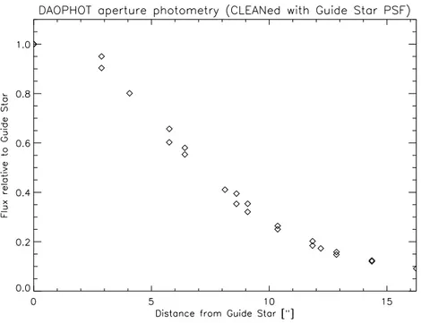
Figure 1.2: Result of aperture photometry on deconvolved image.

guide star). Imaging with a single-layer AO system is therefore anisoplanatic. Of course, even the off-axis performance of AO correction is better than seeing-limited imaging, but many of the data reduction techniques that rely on space-invariance of the PSF have to be used with care on AO corrected images. To illustrate this, a simulation on a very convenient diamond shaped star-field was carried out (details on the parameters used can be found in Chapter 2.3). Figure 1.1 shows a long-exposure image of this simulation; correction was done with measurements on the rightmost star. Two effects are clearly visible: with increasing distance to the guide star, correction quality drops and the PSFs are larger than the diffraction limit; additionally, the off-(correction)-axis PSFs are all elongated in the direction of the guide star. Now, e.g., if an estimate of the relative brightness of the stars is desired, photometry has to be done. There are basically two ways to accomplish this: either PSF or aperture photometry. The first of these assumes that the system PSF is known within a given accuracy, while the second collects flux within an aperture of given size centered on a star. Obviously, both methods rely on a constant PSF, or at least a PSF with a constant size.

In order to show the consequences of “naive” application of these techniques to an AO compensated image, the result of the simulation was first deconvolved using the CLEAN algorithm (H¨ogbom, 1974) and the guide star PSF. The result of this deconvolution is shown in the bottom image of figure 1.1¹. While obviously some improvement has been reached, indicated by the higher contrast and smaller halo of even the most distant stars, both the elongation and the increasing PSF size are still clearly visible. Now, aperture photometry is performed on the CLEANed image, with the aperture size being adapted to the guide star PSF, i.e. the instrument resolution. All stars in the simulation have the same brightness, but, as figure 1.2 shows, photometry delivers a completely different result, with flux estimates relative to the guide star dropping to 10% of the actual value at a distance of 16”. Although this simulation exaggerates a bit, since the chosen atmospheric conditions are comparatively bad (see

1The brighter circular areas around the stars are a consequence of the CLEAN algorithm.

(16)

chapter 2.3), it clarifies the pitfalls of unreflected application of standard photometric techniques to AO assisted imaging.

It should be noted that anisoplanacy is not the only reason for the need to reconstruct the system PSF.

A common situation is that the object of interest lies within the isoplanatic patch but is much fainter than the guide star; in order to achieve a good SNR on the science goal, the guide star has to be heavily overexposed, rendering useless the PSF obtained from its image. Similarly, if the beacon used for correction is not a point source but an extended object (e.g. a LGS, an asteroid etc.), its image is by definition not a PSF.

Goal of this work

The goal of this work is to find a way to reconstruct the on- and off-axis PSF of the ALFA system from wave front sensor signals. For on-axis reconstruction, an algorithm was introduced by Veran et al. (1997) for the PUEO AO at CFHT, using a curvature wave-front sensor. For several reasons (most notably noise estimation), this algorithm has to be modified before being applicable to a Shack- Hartmann type system. Additionally, off-axis reconstruction requires knowledge of the distribution of turbulence throughout the atmosphere, measured simultaneously with AO observations.

(17)

Chapter 2

Turbulence and Adaptive Optics

Atmospheric turbulence is the main source of resolution limitations of ground-based optical and infrared astronomy. Adaptive optics has been devised as a means to overcome these limitations and served this purpose with increasing success over the last decades; however, to use AO enhanced images for scientific ends, a fair knowledge of the properties of the used optical system is mandatory. As these properties are neither space- nor time-invariant for AO systems, this is a non-trivial task.

This chapter will introduce the theoretical concepts necessary to obtain a good estimation of an AO system’s optical properties, depending on controllable (AO system) and non-controllable (atmospheric turbulence) parameters.

We start with a short review of Kolmogorov’s theory of turbulence and its effects on astronomical imaging. Some detail will be given on the first and second order perturbations, i.e. phase variations and scintillation respectively, caused by the atmosphere. In this context the concept of SCIDAR, a means to measure the distribution of atmospheric turbulence, will also be discussed.

The next section deals with the general principle and the setup of a typical AO system. Although other types of sensors will be mentioned, the discussion concentrates on Shack-Hartmann type systems with a modal correction approach, since ALFA follows this design.

Section 2.3 reviews the foundations of on-axis (i.e. guide star) PSF reconstruction by introducing and examining the optical transfer function components contributing to a long-exposure image of a point- like source. Since these concepts were originally conceived for a curvature sensor type AO system (Veran et al., 1997), some differences and problems are to be taken into account. This scheme will then be extended to off-axis PSF reconstruction.

Finally, the example presented in the introduction will be tackled with the instruments developed in the preceding sections, in order to show the improvements possible with a known PSF.

2.1 Effects of Turbulence on Astronomical Imaging

This section starts with a review of Kolmogorov’s theory of turbulence as applied to the atmosphere.

The most important effects of turbulence on wavefronts incident on the earth’s atmosphere are variations in phase due to refractive index fluctuations in turbulent layers and amplitude modulations originating in diffraction at these layers. A very good and complete introduction to these problems can be found in Roggemann and Welsh (1996), a more compact one in the second chapter of Hardy (1998).

Both phase and amplitude modifications caused by turbulence will be examined in separate subsec- tions, with the amplitude subsection extended by a description of a method to measure the vertical

7

(18)

structure of atmospheric turbulence.

2.1.1 Atmospheric Turbulence

The earth’s atmosphere is a system far from equilibrium. The diurnal cycle as well as local variations such as cloud cover, large bodies of water etc. cause differences of the local energy input, which give rise to bulk motions of air. Inside large low or high pressure systems this flow of air is mainly concentrated in horizontal layers. If the Reynolds number of these flows, defined as (with the characteristic length of the flow, its characteristic velocity and the kinematic viscosity

), is higher than one, turbulence will occur. With being typically in the range of m, around m/s and the of air given by , is usually about , so turbulence in airflow is the rule rather than the exception.

Turbulence Models

Kolmogorov developed a simple model for turbulence that describes the distribution of energy in structures (eddies) of different sizes by a power law (Pope, 2000). It is based on the assumption that energy is transferred from large to ever smaller vortexes until the characteristic scale of the very smallest ones reaches a size that lets the Reynolds number drop to the laminar regime where energy is finally dissipated. According to Kolmogorov the distribution of energy in the turbulent structures can

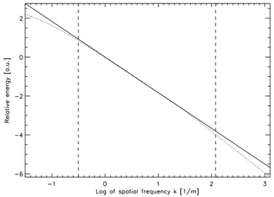
Figure 2.1: Kolmogorov (solid) and von Karman (dotted) turbulence energy spectra. The vertical lines show the limits of the outer and inner scale.

be described by a power law in spatial frequency space,

"!#$

(2.1) with the spatial wavenumber . Obviously this equation is only valid in the case of isotropic turbulence, generally a sensible assumption for the free atmosphere. A more important restriction is the valid range of this energy spectrum, the so-called inertial range, between an outer scale that gives the size of the largest structure and the inner scale^% where turbulent movement finally breaks down.

(19)

2.1. EFFECTS OF TURBULENCE ON ASTRONOMICAL IMAGING 9 The outer scale usually is on the order of meters near the ground up to several tens of meters in the free atmosphere, while the inner scale varies from millimeters to centimeters. This situation is indicated by the dashed lines in figure 2.1. Of course the model of a sharp cutoff in energy at both ends of the power law is quite unnatural. To overcome this problem, the Kolmogorov spectrum has been modified in several ways, the most widely used modification being the von Karman-spectrum, given by

"!

$

(2.2) where and ^% . This spectrum is also plotted in figure 2.1 for the same set of atmospheric parameters as the Kolmogorov one.

Index of Refraction Variations and the Structure Function

The variations in energy and size of the turbulent structures lead to local variations of temperature and pressure in a given turbulent layer. But as the index of refraction of air is a function of those quantities, given by

$

(2.3) where temperature in K and pressure in hPa, turbulence affects the propagation of optical waves through the atmosphere. The refractive index is a passive quantity that has no influence on turbulence itself and it can be shown (Obukhov, 1949) that it follows the same spatial frequency law as the energy distribution; i.e. for the Kolmogorov case

"!$

(2.4) with the refractive index structure constant

. In calculations and simulations, the divergence at

is very inconvenient. Hence, instead of equation 2.4, the structure function of phase fluctuations, or simply phase structure function, (readily deducible from index of refraction fluctuations by Fermat’s principle) is used, given by (Obukhov, 1949)

!

#"

$

!#&%

$

(2.5) This equation gives the average phase difference between two parallel rays of wave number ^$ ^' a distance apart due to a turbulent layer with structure constant

and thickness

% .In the so-called thin layer model, atmospheric turbulence is regarded as being concentrated in a (small) number of layers, usually a ground and a tropopausic layer, sometimes extended by several intermediate layers.

At astronomical observation sites, this model is generally a fair approximation (see also Section 3.3);

in reality however, the atmosphere should be regarded as a continuous turbulent medium, with the structure constant defined as a function of height over the telescopes pupil,

.Thus, the integrated phase difference can be expressed as

(

*)

&+

, -/.

0

!# $

(2.6) with notations as given above and the airmass

)

&+

, inserted to account for viewing directions other than vertical. This equation implies the introduction of the Fried Parameter (Fried, 1965) as

213

)

&+

, - .

54

!#

$

(2.7)

(20)

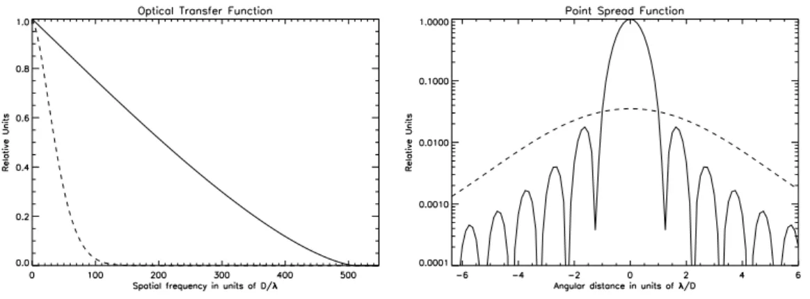
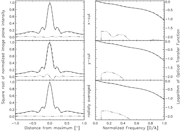
Figure 2.2: Effects of turbulence on image quality for a circular aperture. OTF (left) and PSF (right) of diffraction limited (solid) and turbulence limited (slashes) imaging. was chosen to be 10, resulting in a Strehl ratio (see text) of 0.035 for the turbulence limited case.

which allows Equation 2.6 to be rewritten:

( 1

4 !#

(2.8)

The Fried parameter is a very useful quantity for the characterization of atmospheric turbulence since it has two quite intuitive physical interpretations: first, it gives the size of a (circular) aperture over which the root mean square (rms) of phase aberrations of the incident wavefront is about one radian; second, it defines the minimal diameter of a telescope that will deliver the maximal angular resolution for the given atmospheric conditions. At an observation wavelength of 500 nm, is usually in the range of 5 to 15 cm, much smaller than the typical size of astronomical telescopes. So, in uncorrected long-exposure observations, increasing the diameter of a telescope does not improve angular resolution but only sensitivity by enlarging the gathering area for incoming photons.

With the statistics of phase aberrations known, the effect of turbulence on image quality and telescope performance can now be examined. Two simple approximations and their consequences will be considered in the subsequent sections.

2.1.2 First Order Effects - Geometrical Optics

The first order approximation of imaging through a turbulent atmosphere relies wholly on geometrical optics, i.e. the diffraction of incident waves by turbulent structures is neglected; only the differential retardation of phase between adjacent rays due to the local differences in the index of refraction is taken into account. For good observation sites, this approximation already describes the major part of image degradations introduced by the atmosphere.

Optical Transfer Function

The imaging properties of an astronomical telescope can be fully described by the optical transfer function (OTF) of the system. In the case of imaging through turbulence the total OTF is described by the product of the telescopes’ OTF

, which is just the autocorrelation of its pupil function, and an

(21)

2.1. EFFECTS OF TURBULENCE ON ASTRONOMICAL IMAGING 11 atmospheric OTF , defined by (Roddier, 1981)

"

(2.9)

The PSF of the system is then given by the Fourier transform of the product

. The quantity

in equation 2.9 of course not only refers to the phase structure function given in equation 2.6 but to any phase structure function that can be defined on a telescope pupil. This will be of further importance when looking at partially corrected wavefronts as produced by adaptive optics systems. For the time being, figure 2.2 shows the effects of (Kolmogorov) turbulence on the imaging performance of an astronomical telescope with a circular aperture. In this example, the ratio has been chosen to be 10. As can be seen, the OTF drops to zero much faster than in the diffraction limited case, resulting in the filtering of high spatial frequencies. The consequence is that the peak intensity of the PSF is considerably flattened and its FWHM strongly increased. It should be noted that these results are valid for long-exposure imaging only, since,in equation 2.9, the ensemble average of phase aberration realizations is given. Short-exposure imaging depends very much on the momentary configuration of the phase in the pupil plane, which leads to an OTF that also transports high spatial frequency information. This fact is exploited by Speckle imaging techniques (Labeyrie, 1970), see also figure 2.4.

Strehl Ratio

Figure 2.2 also serves to introduce another useful quantity to characterize the performance of an imaging system: the Strehl ratio (Strehl, 1902). It is defined by the ratio of the actual peak intensity

to the theoretical (i.e. diffraction limited) peak intensity of the PSF, . If the aberration function ^$ of an optical system is given, the Strehl ratio can be calculated via (Hardy, 1998)

-

!"

0 0 (2.10)

A problem of this equation is that the aberration function has to be known explicitly, whereas in uncompensated and compensated astronomical imaging the phase fluctuations are at best known sta- tistically. Therefore several simplifications of equation 2.10 have been found, notably the widely-used Marechal approximation given by

$#

%'&("*)

$

(2.11) where^,+ is the standard deviation of the phase over the aperture (Hardy, 1998). The Marechal approximation is valid up to an phase rms of about 2 rad. Turbulence degraded wavefronts are mostly well above this limit, hence a simple expression for this case is not available.

Anisoplanacy

Another important geometrical effect of imaging through a turbulent atmosphere is angular anisopla- natism. It is a consequence of the fact that rays from different viewing directions will pass through different sections of the atmosphere (see figure 2.3). While in uncompensated imaging anisoplanacy is only significant in short-exposure observations, it is a big problem for adaptive optics. Using equation 2.6 as a starting point and assuming

" " , the mean-square error

! "

due to anisoplanacy can be calculated by replacing with

)

&+

, , where as shown in figure 2.3. This calculation yields

! "

)

&+

, .-

!# !#

- . !#

(2.12)

(22)

Image Plane

Projected Pupil

Upper Layer

Intermediate Layer

Ground Layer

α

Figure 2.3: The origin of anisoplanacy. Incident plane waves from directions that are an angle apart pass through different sections of turbulent layers above ground.

Similar to the definition of the Fried parameter, it is possible to define an angle

as

)

&+

, -

!#

- .

0

!#

$

(2.13)

such that

! " 1

4 !#

(2.14)

is called the isoplanatic angle; its interpretation corresponds to that of , defining the angular distance between two sources at infinity for which the difference in phase aberrations is approximately 1 rad. In contrast to the Fried Parameter, however, that is only dependent on the total integrated structure function, the isoplanatic angle shows a strong dependency on the vertical structure of the turbulence profile. As one would naively expect, high turbulent layers contribute strongly, while layers at or near ground level have virtually no influence on the differential error of two incident wavefronts.

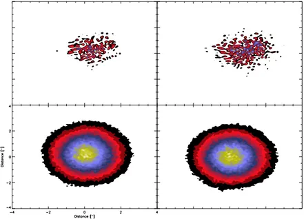
To illustrate the effect of anisoplanacy on uncorrected imaging, the simulation package TURBULENZ (App. A) was used to calculate short and long exposure images of two stars about 12 arcseconds apart;

the applied turbulence model was chosen such as to result in an isoplanatic angle of 8 arcseconds.

Figure 2.4 shows the results: while the short-exposure (speckle) images are clearly different, the overall shape and size of the long-exposure images is about the same. It is also visible that the speckle images contain much higher spatial frequencies than the integrated ones; the reason for which was already mentioned in section 2.1.1.

(23)

2.1. EFFECTS OF TURBULENCE ON ASTRONOMICAL IMAGING 13

Figure 2.4: Short (top) and long-exposure (bottom) images of two stars 12 arcseconds apart in turbulent conditions corresponding to .

Temporal Effects

Up to now, the temporal evolution of turbulence was largely ignored, only ensemble averages of instantaneous realizations of phase disturbances were considered. Under real observing conditions, however, temporal effects cannot be disregarded.

Usually the validity of the Taylor hypothesis of frozen flow is assumed, stating that the structure of turbulence itself is fixed while the corresponding section of the layer is moving through the viewing area of the telescope. While this is generally a good approximation for smaller telescopes up to a pupil diameter of four meters, evolution of these structures does play a role for larger observatories.

For a single layer moving at constant speed the Taylor hypothesis can be formally stated by

$ %

%$

$

(2.15) resulting in a temporal phase structure function

$

% $

" (2.16)

This equation translates temporal evolution into spatial distances. Note that this introduces anisotropy into the phase structure function, dependent on the direction of wind. If exposure times are short (or long) enough, however, these effects will be negligible. Long enough means that any correlations present on the medium time scale (several tens of ms) cancel out in the long-term limit, while short enough can be quantified by the Greenwood frequency (Greenwood, 1977), a measure of the required bandwidth for any attempt to measure sensible wavefront aberrations. For a single turbulent layer, is given by , while for a turbulence distribution

)

&+

, - .

!# !#

$

(2.17)

(24)

with the vertical wind speed profile (Greenwood, 1976). As an example, typical tropopausic layer conditions with wind speeds on the order of and an of in the K-Band result in a required bandwidth of Hz, a demand easily met by modern sensors and control systems.

2.1.3 Second Order Effects - Scintillation and SCIDAR

Although the geometrical approximation described in the previous section already accounts for the major part of turbulence effects on imaging through the atmosphere, wave diffraction does of course also take place. Its most prominent influence on astronomical imaging is that of scintillation, the origin and features of which will be explained in this section. As turbulence at astronomical sites is generally quite weak, the so-called Rytov approximation can be used.

The Rytov Approximation

It has been shown quite early (Bergmann, 1946) that the assumption of geometrical optics is not sufficient if propagation path lengths are in excess of ^%

; then, diffraction effects at turbulent eddies have to be taken into account. In principle it would be necessary to solve the Maxwell equation

$

(2.18) for the electric field and the local deviation of the index of refraction from unity, . Dropping the last term (depolarization) and substituting

yields

(2.19)

Now, is substituted by ^# , where represents the non-fluctuating component (the incident wave) and describes fluctuation due to turbulence. If is neglected in comparison to

and

in comparison to then satisfies

# $

(2.20) which has a solution given by Fante (1975)

-!- - 0

$

(2.21) where

. This solution has a much wider range of applicability than the geometrical one. It has been found (Gracheva et al., 1970) that if the propagation path is such that the Rytov variance

!

"!

is smaller than 0.3, the Rytov approximation is excellent. Equation 2.21 has a very simple physical interpretation that states that the Rytov approximation is equivalent to independent diffraction of the incident wave at a series of turbulent phase screens (Lee and Harp, 1969), i.e. inclusion of multiple diffraction is not necessary. A very important point to note is that the form of the phase structure function in equation 2.6 statistics is not changed at all, since the phase

is still proportional to . The amplitude of an incident plane wave, however, which is constant under the geometrical approximation, is strongly affected; a closer look at the consequences will be taken in the subsequent paragraphs.

(25)

2.1. EFFECTS OF TURBULENCE ON ASTRONOMICAL IMAGING 15 Intensity Fluctuations in an Aperture

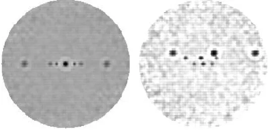
Figure 2.5 shows intensity fluctuations in an image of the aperture of the Calar Alto m telescope.

The best characterization of these fluctuations can be found by calculating the covariance of the loga- rithm of the amplitude fluctuations at two aperture locations and ,

$ " $

with

.

$ is related to the intensity fluctuations (Fante, 1975)

$

" "

"

" (2.22)

via

$

(2.23)

For the case of an incident plane wave, is given by (Fante, 1975)

-/.

0 -/.

0

$ )

$

(2.24) with , spatial frequency , as defined in equation 2.4, and the distance of the turbulence from the aperture plane of the telescope.

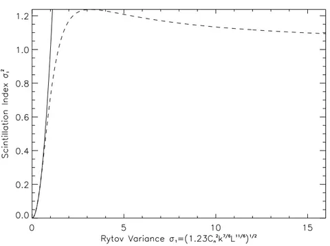
Figure 2.6 plots the Rytov variance against the scin-

Figure 2.5: Intensity fluctuations in the aperture plane of the Calar Alto 1.23m telescope.

tillation index for the Rytov theoretical results and experimental data (Fante, 1975). The theoretical results for an infinitesimally small aperture are obtained by calculating ^$ using equation 2.24. It is obvious that the Rytov approximation is in excellent agreement with measurements for

while it completely fails to describe the sat- uration behavior of scintillation in severe turbulence.

However, astronomical sites usually are well below the upper limit of validity of the Rytov approximation (see also chapter 3.3). For completeness’ sake it should be mentioned that analytical approximations

for strong turbulence also exist, most notably the Markov approximation (Tatarski, 1971), which is e.g. used in calculation concerning horizontal laser beam propagation.

Effects on Imaging

Many of the relations presented in the previous paragraph are only valid for an infinitesimally small aperture. If effects of scintillation on imaging are considered, however, aperture averaging has to be taken into account. To derive the brightness fluctuations of the image of a star in the image plane of a telescope, one therefore calculates

#"

- - 0 - - 0 $ $

(2.25) where integration is carried out over the pupil of the telescope. Aperture averaging basically results in easing the effect of scintillation, since locations well inside the aperture do not contribute to the

(26)

Figure 2.6: Scintillation index measured in an infinitesimal aperture. Rytov approximation (solid) and fit to measured values (dashed).

integrated brightness fluctuations any more. Only points near or at the fringe of the pupil have consid- erable influence; thus a significant reduction of the magnitude of fluctuations is expected for growing aperture size, a fact many times experimentally confirmed (Homstad et al., 1974).

Intensity fluctuations are, however, not the only effect of scintillations, a bigger problem is posed by their influence on the system OTF. Roddier and Roddier (1986) showed that even if phase aberrations caused by turbulence are perfectly removed, a performance degrading OTF term

!#

)

&+

, "!

' ! -/.

0 !

+

)

,

'

"! $

(2.26) remains, where is the normalized

profile and

- .

0 -

!#

)

$

(2.27) with the Bessel function of order zero. Its overall effect is a limit on the maximum Strehl ratio obtainable by phase correction, given by the asymptotic value of the scintillation OTF term. For infrared imaging, this limitation is negligible, in the visual band it can be as low as 0.8.

2.1.4 Measuring : SCIDAR The vertical structure of

is the determining factor for many imaging distortions caused by the turbulent atmosphere. Therefore, it is highly desirable to obtain time-resolved information on it, either for image post-processing purposes or even for the selection of sites suitable for astronomical observatories. Although atmospheric sounding or weather balloons have been used to this end, another technique has proved its potential in this important task: Scintillation Detection and Ranging

(27)

2.1. EFFECTS OF TURBULENCE ON ASTRONOMICAL IMAGING 17

Pupil Plane Pupil Plane)

Camera (Image of

SCIDARSCIDAR

Generalized

hgs(f T , f , f

gs) 0

f

f f

f T

T 0

gs

low Pupil Plane Pupil Plane)

Camera (Image of

high altidude turbulence

Figure 2.7: Setup of a SCIDAR and a generalized SCIDAR system.

(SCIDAR). The principle of this method was developed by Vernin and collaborators (Vernin et al., 1979) and has since been much enhanced, notably by the generalized SCIDAR approach (Fuchs et al., 1998). In this section, the setup of a typical SCIDAR system will be described before looking at the kind of data obtainable with such a device and the information on atmospheric turbulence derivable from it.

SCIDAR system setup and measurements

Figure 2.7 shows the configuration of a SCIDAR system. Its working principle builds on the amplitude variations imposed on plane waves imaged through the atmosphere, as described in the previous section. As shown in the figure, light originating from binary stars passes through different sections of the atmosphere. If the binary is chosen such that the cross-sections of the projected pupils overlap at all heights of interest, the spatial amplitude patterns of the overlap region as measured on the aperture will be the same albeit shifted by

%

with respect to each other, with the distance of the layer and the angular separation of the binaries. However, the amplitude variations comprising those patterns need a distance of a few kilometers to build up to a measurable signal, thus measuring turbulence near or at ground level is impossible with SCIDAR. Fuchs et al. (1998) found a way to overcome this limitation, by placing a different lens into the optical path such that the conjugate height of the observation plane is shifted from the pupil to a plane virtually below it (see figure 2.7). This extension is known as generalized SCIDAR.