A Shortcut to the Q-Operator

arXiv:1005.3261v2 [hep-th] 4 Jun 2010

AEI-2010-023 HU-EP-10/24 HU-Mathematik: 2010-7

A Shortcut to the Q-Operator

Vladimir V. Bazhanov ^a, Tomasz Lukowski ^b,c, Carlo Meneghelli ^c, Matthias Staudacher ^c,d

a Department of Theoretical Physics, Research School of Physics and Engineering Australian National University, Canberra, ACT 0200, Australia

b Institute of Physics, Jagellonian University ul. Reymonta 4, 30-059 Krak´ow, Poland

c Max-Planck-Institut f¨ur Gravitationsphysik, Albert-Einstein-Institut Am M¨uhlenberg 1, 14476 Potsdam, Germany

d Institut f¨ur Mathematik und Institut f¨ur Physik, Humboldt-Universit¨at zu Berlin Postal address: Unter den Linden 6, 10099 Berlin, Germany

Vladimir.Bazhanov@anu.edu.au tomaszlukowski@gmail.com

carlo@aei.mpg.de matthias@aei.mpg.de

Abstract

Baxter’s Q-operator is generally believed to be the most powerful tool for the exact diago- nalization of integrable models. Curiously, it has hitherto not yet been properly constructed in the simplest such system, the compact spin-¹₂ Heisenberg-Bethe XXX spin chain. Here we attempt to fill this gap and show how two linearly independent operatorial solutions to Baxter’s TQ equation may be constructed as commuting transfer matrices if a twist field is present. The latter are obtained by tracing over infinitely many oscillator states living in the auxiliary channel of an associated monodromy matrix. We furthermore compare and differentiate our approach to earlier articles addressing the problem of the construction of the Q-operator for the XXX chain. Finally we speculate on the importance of Q-operators for the physical interpretation of recent proposals for the Y-system of AdS/CFT.

1 Motivation

Recently there was much progress with integrability in planar four-dimensional gauge the- ories [1, 2, 3] and AdS/CFT [4, 5]. At variance with the long-held belief that quantum integrability is confined to low-dimensional systems, the asymptotic Bethe Ansatz solu- tion of planar N = 4 gauge theory was conjectured by a combination of rigorous results and assumptions [5]. Further conjectures and arcane techniques led to first proposals [6]

for the full, non-asymptotic spectrum of this gauge theory, as well as its dual superstring theory on the space AdS₅×S⁵. The proper interpretation and even the veracity of these latter proposals remains hotly debated, and in any case there is currently no trace of the theoretical underpinnings of the employed experimental mathematics. The final equations obtained take the form of an infinite system of integro-difference equations, based on a conjectured thermodynamic Bethe Ansatz, which involve an infinite set of “T-functions”.

These may in turn be rewritten for a sometimes more convenient set of “Y-functions”.

In the large volume limit the “T-functions” are to be interpreted as transfer matrices of an infinite number of excitations, most of them corresponding to bound states. However, some of the T-functions involve excitations believed to be elementary (mirror-magnons), while others turn into what looks like the eigenvalues of some Baxter Q-operators.

It is currently totally unclear which operators T and Q possess all these eigenvalues T and Q. In other words, even if the proposals [6] are made more precise, and turn out to be correct, the question “What has been diagonalized?” will remain unanswered.

One clearly would like to construct the associated operators, and prove that their mutual commutativity is based on an underlying Yang-Baxter symmetry.

One very curious feature of AdS/CFT integrability is that the underlying integrable system is both a quantum sigma-model “living” on a smooth continuous two-dimensional worldsheet, and at the same time a certain long-range spin chain defined on a discrete lattice. The two pictures are related by a continuous coupling constant, and one cannot say that the continuum sigma model is obtained from a discrete spin chain by a continuum limit. The sigma model isalso a spin chain.

For short-range spin chains, the construction of transfer matrix operators T is rather well understood, see below. However, the general principles of construction of the Baxter Q-operators, originally introduced in his seminal paper on the 8-vertex model [7], are less well understood, and appear to be less systematic, even though the subject was intensively studied for the past twenty years. An important step toward a general algebraic theory of the Q-operators, particularly relevant for this paper, was made in [8, 9] devoted to confor- mal field theory where these operators were constructed as traces of certain monodromy matrices, associated with infinite dimensional representations of the q-deformed harmonic oscillator algebra. More generally this method applies to any model withUq(sl(2)) symme-b try and it was further generalized for the case of some higher-rank quantized algebras and super-algebras [10, 11, 12]. However despite all these considerations of rather complicated models with “q-deformed” symmetries, it appears that there is still no proper construction in the literature for theQ-operator of the compact XXX chain — the first spin chain ever solved by Bethe Ansatz [13]. We therefore decided to fill this gap, as a very first neces-

sary step to vigorously address the much more involved case of AdS/CFT integrability.

Excitingly, we will find that we need infinite dimensional representations to carry out this construction. These are therefore needed to properly understand the integrable structure of spin chains with finite dimensional quantum space, a feature which then puts spin chains on a par with integrable sigma models. We believe that this makes the appearance of spin chains in the strongly coupled limit of the AdS/CFT sigma model much less surprising.

2 Brief Review of the Spin-

XXX Heisenberg Chain

The one-dimensional Heisenberg spin chain Hamiltonian reads H= 4

XL l=1

1

4−S~l·S~l+1

with S~= 1

2~σ , (2.1)

where ~σ are the three Pauli matrices, i.e. S~ is the spin-¹₂ representation of su(2). This Hamiltonian acts on the L-fold tensor product

V =C² ⊗C² ⊗ · · · ⊗C²

| {z }

L−times

, (2.2)

which will be called quantum space throughout the paper. The spin operator S~^l acts on thel-th component of the quantum space, and it is clear from (2.1) that we need to specify the meaning ofS~^L+1. Periodic boundary conditions are imposed by defining

S~L+1 :=S~1. (2.3)

This Hamiltonian may be rewritten as H = 2PL

l=1(I_l,l+1−P_l,l+1) where I_l,l+1 and P_l,l+1 are the identity and the spin permutation operators on adjacent sites (l, l+1) of the chain of lengthL, respectively. It appears in N = 4 Yang-Mills theory in the scalar field subsector, where S ∈~ su(2) ⊂ su(4) ⊂ psu(2,2|4), as the one-loop approximation of the conformal dilatation generator D ∈su(2,2)⊂psu(2,2|4)

D =L+g²H+O(g⁴). (2.4)

Here g² is related to the ‘t Hooft coupling constant λ by g² = _16π^λ2. Note that the Hamil- tonian (2.1) with boundary conditions (2.3) is rotationally invariant, i.e. [H, ~S] = 0.

It is well known that Hans Bethe discovered in 1931 a system of algebraic equations which yield the exact spectrum of H. This was obtained after making an Ansatz for the wave function now carrying his name [13]. This so-called coordinate Bethe Ansatz interprets the state↑. . .↑with energy eigenvalueE = 0 as the vacuum. Each up-spin↑ is an unoccupied lattice site, and each down-spin↓is interpreted as a lattice particle, termed magnon, carrying lattice momentum p. After introducing a rapidity u for each magnon, where

e^ip = u+ ₂ⁱ

u− ₂ⁱ ⇐⇒ u= 1 2cotp

2, (2.5)

Bethe’s solution for the eigenvalues E of H in the (conserved) sector ofM magnons reads E = 2

XM k=1

1

u²_k+¹₄ , (2.6)

where the M Bethe roots uk have to satisfy the Bethe equations uk+ ₂ⁱ

uk− ₂ⁱ L

= YM

j=1

j6=k

uk−uj+i

uk−uj−i. (2.7)

The eigenvalue U of the lattice translation operator U, which shifts a given spin configu- ration by one lattice site, is given by

U = YM k=1

uk+ ₂ⁱ

u_k− ₂ⁱ . (2.8)

There has been a longstanding controversy, starting from a discussion in Bethe’s original paper, as to whether the obtained spectrum is complete, which still attracts much attention;

here we give only a small sample of references [14, 15, 16, 17]. There are (at least) three distinct subtleties. The first is, that the map (2.5) leads to infinite rapidities u = ∞ for zero-momentum magnons wherep= 0. Of course this is consistent with both the expression for the energy (2.6) and the Bethe equations (2.7), but complicates the proper counting of states. The effect may be traced to the su(2) invariance of H: The highest weight state of each energy multiplet corresponds to a solution with only finite rapidities. The descendents of this state are obtained by applying the globalsu(2) lowering operator. Each application places a further p = 0 magnon into the chain, corresponding to a completely symmetrized insertion. A second subtlety is that it is a priori not allowed to increase M beyond half-filling, i.e. such thatM > L/2 (all states must then be descendents). Spurious states with finite rapidities are nevertheless found. In fact, one “experimentally” finds that solving the equations

u˜k+ ₂ⁱ

˜ uk− ₂ⁱ

L

=

L−MY+1

j=1

j6=k

˜

uk−u˜j +i

˜

u_k−u˜_j −i (2.9)

for L−M + 1 roots ˜uk and plugging the solution into E = 2

L−M+1X

k=1

1

˜

u²_k+¹₄ (2.10)

yields energies identical to the ones of highest weight states with magnon number M.

However, the root distribution ˜uk = ˜uk(α) depends on one arbitrary complex parameterα, while the energy does not. These “beyond the equation solutions” were discussed in detail in [18]. The third subtlety, already noted in [13], is that some momenta appear in pairs

of the form p = p0±i∞, which leads via (2.5) to Bethe roots at u = ±₂ⁱ. The physical picture here is that two magnons form an infinitely tight bound state¹, they are “stuck together”. However, they of course contribute only a finite amount of energy, so (2.6) has to be interpreted with great care.

It is also quite well known that all these subtleties may be resolved by replacing H by a “twisted” Hamiltonian H_φ, where φ can be interpreted as an (imaginary) “horizontal field” in condensed matter parlance, or alternatively as a magnetic flux passing through the chain looped into a circle

Hφ= 4 XL

l=1

1

4 − Sl³Sl+1³ − 1

2e^iφLSl⁺Sl+1⁻ − 1

2e^−iφLSl⁻Sl+1⁺

, (2.11)

withSl^± =Sl¹±iSl². The Bethe Ansatz still works with minor modifications. The formula for the energy (2.6) and the relations (2.5) remain unaffected, but the Bethe equations (2.7) are modified to

uk+₂ⁱ u_k−₂ⁱ

L

e^iφ = YM

j=1

j6=k

uk−uj +i

uk−uj −i. (2.12)

This tiny modification resolves all the difficulties we just discussed (for generic values of the twist). Firstly one now finds all 2^L states of the length L spin chain, such that all rapidities uk are finite. Secondly, there is no “beyond the equator problem” anymore and M can range over M ∈ {0,1, . . . , L −1, L}. In fact one can now rigorously derive the second Bethe Ansatz, which treats the up-spins as “dual” magnons in the vacuum of the down-spins. It reads

u˜k+ ₂ⁱ

˜ uk− ₂ⁱ

L

e^−iφ=

L−MY

j=1

j6=k

˜

uk−u˜j+i

˜

uk−u˜j−i, (2.13)

E = 2

L−MX

k=1

1

˜

u²_k+¹₄ , (2.14)

and in contradistinction to (2.9),(2.10) there are only L−M dual magnons, as expected.

In fact, the set of equations (2.12) and (2.13) are completely equivalent, each set yields the full spectrum of all 2^L states. Finally there are no more degenerate roots at u = ±₂ⁱ with a priori indefinite energy (2.6) or (2.14). The price to pay is that su(2) invariance of the spectrum is broken: All multiplets split up². However, we can think of φ as a small regulator which may always be removed where physically sensible. Note that such twists are also natural from the point of view of the AdS/CFT correspondence. They appear in the scalar sector of the integrable one-loop dilatation operator of the β-deformed twisted N = 4 gauge theory [19].

1This happens first for one of the two singlet states of theL= 4 spin chain.

2A spins multiplet where the magnetic quantum numbers are m =−(2s+ 1), . . . ,(2s+ 1) splits up such that there still is a degeneracy between any two states whosem differs by a sign flip.

The magnetic flux φ may be distributed in many possible ways. For instance, as concerns the energy spectrum of the spin chain, it is equivalent to use instead of (2.11) a linearly transformed Hamiltonian,

Heφ=C φ/L

HφC φ/L−1

, C(α) =e^{i LαSL3} ⊗e^{i(L−1)αSL3−1} ⊗ · · · ⊗e^{i αS13} , (2.15) which is given by the original formula (2.1), but with “twisted” boundary conditions

SL+1³ :=S1³, SL+1^± :=e^∓iφS1^±. (2.16) There is an interesting way to reformulate the Bethe equations (2.12) and (2.13) with the help of Baxter polynomials defined for each eigenstate by

A−(u) :=

YM k=1

(u−uk), A+(u) :=

L−MY

k=1

(u−u˜k). (2.17) Then

u+₂ⁱ u− ₂ⁱ

L

e^±iφ =−A∓(u+i)

A∓(u−i) if u=u_k or u= ˜u_k, respectively. (2.18) On infers that the following equations must hold for each eigenstate and for all u∈C:

T(u)A∓(u) =e^±iφ2

u+ i 2

L

A∓(u−i) +e^∓iφ2

u− i 2

L

A∓(u+i). (2.19) The reason is that the r.h.s. is a polynomial with roots atu=ukoru= ˜uk, respectively, so it must be proportional toA∓(u). We also see that the latter function must be multiplied by another polynomial T±(u) of degree L. One experimentally finds that this further polynomial does not depend on ±, i.e. T±(u) = T(u), a fact which will be proven in the next chapter. So we have from (2.19) and (2.17)

T(u) = 2 cosφ 2

YL k=1

(u−wk), (2.20)

where the wk are the remaining Lroots of the r.h.s. of (2.19).

Equation (2.19) can be regarded as a second order difference equation for an unknown function A(u), which has two linearly independent solutions A±(u). To see this more clearly, it is convenient to define the Baxter functions

Q±(u) :=e^±uφ2 A±(u), (2.21) such that Q±(u) are indeed two linearly independent solutions³ of the difference equation

T(u)Q(u) =

u+ i 2

L

Q(u−i) +

u− i 2

L

Q(u+i) with Q(u) =Q±(u). (2.22)

3The most general formal solution of (2.22) is then a linear superposition of the form Q(u) = c+(u)Q+(u) +c−(u)Q−(u). However, unlike the theory of second order differential (as opposed to differ- ence) equations is that the “constants”c±(u) could a priori be any functions ofuwith periodi.

This is Baxter’s famousT Qequation for the twisted Heisenberg magnet. As we can see, the twist has actually disappeared from the equation, and is entirely encoded in the analytic Ansatz (2.21),(2.17),(2.20) for the solution. Note that the Baxter functions at nonzero twist φ are not polynomials.

Baxter derived this equation, which holds for all eigenvalues of the commuting T- and Q-matrices on the operatorial level, in his original solution on the “zero-field” 8- vertex model [7], which also contains the solution of the “zero-field” XYZ spin chain [20].

Although it seems to be possible to take a limit of his results and apply them to the untwisted XXX model, this would then only apply to the “zero-field” case φ = 0.

One purpose of this article is to consider the XXX chain with an arbitrary non-zero field φ 6= 0 and provide an independent construction of the operators T(u) and Q±(u) satisfying (2.22) such that all their eigenvalues are of the form spelled out in (2.21), (2.17) and (2.20). Our construction of the Q-operators is conceptually very similar to that of [8, 9] in c < 1 conformal field theory, based on the Yang-Baxter equation with Uq(sl(2))b symmetry. However, here we provide a self-contained and separate consideration of the XXX model, rather than attempting to take the q² → 1 limit of the relevant results of [8, 9].

In the case of the operator T(u) Baxter’s construction actually immediately applies.

His methodology was subsequently developed and systematized by the inverse scattering methodology of the Leningrad school of mathematical physics. Here we will just briefly summarize the construction, referring for all further details to the authoritative presenta- tion [21]. One constructs this operator, termed transfer matrix T(u), as the trace over a certain monodromy matrix M(u). The latter is in turn built from a “generating object”, the local quantum Lax operator

Ll(u) =

u+iSl³ iSl⁻

iSl⁺ u−iSl³

, (2.23)

which is a 2×2 matrix in some auxiliary space C² with site-l spin operator (as in (2.1)) valued matrix elements. The monodromy matrix is then built as⁴

M(u) = e^iφ2 0 0 e^−iφ2

!

· L^L(u)· L^L−1(u)·. . .· L²(u)· L¹(u). (2.24) In view of (2.2) it is an operator acting on the tensor product of the auxiliary space and the quantum space. Finally, by taking the trace over the two-dimensional auxiliary space, T(u) = TrM(u), (2.25) one constructs the transfer matrix as an operator on the quantum space (2.2). It is easy to show, see [21], that at the special point u= ₂ⁱ the transfer matrix becomes proportional

4Here·denotes 2×2 matrix multiplication in the two-dimensional auxiliary space. The entries of this 2×2 matrix act on (2.2).

to the lattice shift operator (cf. discussion around (2.8)), multiplied by a diagonal matrix, i.e. one has

U =i^−LT(₂ⁱ)e^{−i φ SL3} . (2.26) The Hamiltonian (2.15) is then obtained from the expansion of the transfer matrix in the vicinity of the point u= ₂ⁱ ,

He_φ= 2L−2i d

dulogT(u)

u=₂ⁱ . (2.27)

Finally, because of the underlying Yang-Baxter symmetry, to be discussed below, one can show that transfer matrices with different values of spectral parameters form a commuting family

[T(u),T(u^′)] = 0, (2.28)

which also contains the Hamiltonian (2.15), obtained from (2.1) by twisting the boundary conditions (2.16). However, this fact by itself does not directly lead to the solution of the model. One procedure is to apply the algebraic Bethe Ansatz as explained in [21].

Another, to be developed below, is to also construct the operators Q±(u) as traces over some monodromy matrices, and to derive the operator version of (2.22)

T(u)Q±(u) = u+₂ⁱL

Q±(u−i) + u− ₂ⁱL

Q±(u+i), (2.29) along with a proof that the analyticity of the eigenvalues of the therein appearing operators is given by (2.21),(2.17),(2.20). Then no Bethe Ansatz is required, and the twisted Bethe equations (2.12) or (2.13) immediately follow (for more details on this logic, please see section 3.5 below).

A very interesting issue is the φ→0 limit of the operators Q±(u) appearing in (2.29).

In this limit, the brokensu(2) invariance of the spin chain is recovered. Then the majority of the eigenvalues of Q±(u) turn into descendents of su(2) highest weight states. From our discussion following the untwisted Bethe equations (2.7) these will have Bethe roots at u=∞, so the operatorsQ±(u) are expected to diverge, in stark contrast to the eigenvalues of T(u), which are perfectly finite and smooth in the zero-twist limit. On the other hand, we can of course retrace the steps leading to the existence of the operator equations (2.29) by making, in analogy with (2.17), a polynomial Ansatz for linearly independent Baxter functions⁵

Q(u)∼ YM k=1

(u−u_k), P(u)∼

L−MY+1 k=1

(u−u˜_k). (2.30) This empirical way had already been explored in [18], but it was erroneously (as we shall see) stated that P(u) and Q(u) are completely unrelated to the eigenvalues of Q±. By using the untwisted Bethe (2.7) and dual Bethe (2.9) equations, the latter being the reason for the power L−M + 1 in the polynomial P(u), we conclude that there must be finite

5Note that the exponential factors in (2.21) disappear at φ= 0. We have used the notation ∼since the proper normalization of these functions will turn out to be quite subtle.

operatorsQ(u),P(u) which should satisfy thesameBaxter equation (2.29) asQ±(u), such that however (1) their eigenvalue spectrum issu(2) invariant, and (2) their eigenvalues are indeed of the form in (2.30). It is clear that finding Q(u),P(u) from Q±(u) must indeed be quite non-trivial, and must involve some kind or “renormalization” of these divergent operators. It is furthermore a priori quite mysterious how the extra (L−M + 1)-th root appears inP(u) in (2.30) as compared to theL−M roots ofA₊(u) in (2.17). These puzzles will be resolved in chapter 4. In particular, we shall find the resolution to be intimately connected to the exponential factors in (2.21).

Our article is organized as follows. In the ensuing chapter 3 we will construct the operators Q± as the trace over an appropriate monodromy matrix. This will require the introduction of two copies of infinite oscillator Fock spaces, despite the fact that we are dealing with a finite dimensional spin chain carrying finite dimensional representations of su(2). In the next chapter 4 we will study the very subtle φ→0 limit of our construction, leading to a one-parameter family of linearly independent operatorsQ(u),P(u) by “renor- malizing” the previously obtained operators Q±. We will also perform some numerical study of their spectrum for a few cases, illustrating an interesting pattern between their respective eigenvalue root distributions. In the following chapter 5 we briefly discuss how our construction and result differ from a large earlier, complementary literature on the sub- ject. We end in 6 with a brief list of the many open problems and potential applications related to our result.

Before proceeding with the construction of the operators Q±, let us however change notation by “Wick-rotating” the spectral parameter u to

z :=−i u . (2.31)

It is true that theu-convention of this review chapter 2 is the most widely accepted notation in much of the Bethe Ansatz literature, and nearly all of the literature on AdS/CFT integrability. But thez-convention (2.31) used for the rest of this paper (with the exception of the numerical work presented in section 4.5 and appendix F, as well as the examples of small chain lengths in appendix B) prevents all further derivations and manipulations of functional equations from being cluttered by factors of i. This will then turn (2.29) into⁶

T(z)Q±(z) = z+¹₂L

Q±(z−1) + z− ¹₂L

Q±(z+ 1). (2.32)

3 Construction of Q

as Transfer Matrices

3.1 Yang-Baxter equation and commuting transfer matrices

As explained above the Hamiltonian (2.1), with twisted boundary conditions (2.16), is generated by the spectral parameter-dependent transfer matrices (2.25), which form a

6For simplicity, and with slight abuse of notation, we will not use new symbols for the various operators.

E.g. the transfer matrix in (2.29) is i^L times the transfer matrix in (2.32). It should be straightforward to return to the notation with the spectral parameteruwhenever needed by using (2.31).

commuting family, cf. (2.28). Here we want to construct further important transfer matrices which nevertheless belong to the same family. To this end one needs to study the possible solutions of the Yang-Baxter equation

R(x−y) L_V(x)⊗1

1⊗L_V(y)

= 1⊗L_V(y)

L_V(x)⊗1

R(x−y), (3.1) where R(z) is the rational 4×4 R-matrix,

R(z) : C²⊗C² →C²⊗C², R(z) =z+P, (3.2) and theL-operatorL_V(z) is a 2×2 matrix, acting in the quantum space of a single spin-¹₂,

L_V(z) =

L₁₁(z) L₁₂(z) L₂₁(z) L₂₂(z)

. (3.3)

Its matrix elements are operator-valued functions of the variable z, acting in an auxiliary vector space V. The R-matrix acts in a direct product of two-dimensional spaces C²⊗C² and the operator P permutes the factors in this product. Note that the R-matrix (3.2) is GL(2)-invariant

R(z) = (G⊗G)R(z) (G⊗G)⁻¹, G∈GL(2), (3.4) where Gis any non-degenerate 2×2 matrix.

The solutions of (3.1) which we will use in this paper are rather simple. The first one is a well-known generalization of (2.23),

L(z) =

z+J³ J⁻ J⁺ z−J³

=zI+ 2 X3

k=1

S^kJ^k, (3.5)

where J^± =J¹±iJ² and J³ are the generators of thesl(2) algebra J³,J^±

=±J^±,

J⁺,J⁻

= 2J³. (3.6)

In the second form ofL(z) in (3.5) we used the 2×2 spin operatorsS^k appearing in (2.1).

Note that for theL-operator (3.5) equation (3.1) holds on the algebraic level in virtue of the commutation relations (3.6). To obtain a specific solution one needs to choose a particular representation of these commutation relations. For further reference define the highest weight representions of sl(2), with highest weight vector v0, defined by the conditions

J⁺v0 = 0, J³v0 =j v0, (3.7)

where j is the spin. The (2j+ 1)-dimensional representations with integer or half-integer spin, i.e. 2j ∈ Z_≥0, will be denoted by π_j, while infinite-dimensional representations with arbitrary complex spin 2j ∈Cwith be denoted as π_j⁺.

For each solution of (3.1) one can define a transfer matrix T_V(z) = TrV

D L_V(z)⊗L_V(z)⊗ · · · ⊗L_V

| {z }

L−times

, (3.8)

where the tensor product is taken with respect to the quantum spacesC², while the operator product and the trace is taken with respect to the auxiliary spaceV. The boundary twist operator D, specially suited for our purposes, is defined by

[D, L₁₁(z) ] = [D, L₂₂(z) ] = 0, D L₁₂(z) =e^iφL₁₂(z)D, D L₂₁(z) =e^−iφL₂₁(z)D, (3.9) where L_ij(z), i, j = 1,2, denotes matrix elements of L_V(z). Note that D is an operator in the auxiliary space; it acts trivially in quantum space⁷. For the solution (3.5) one easily finds

D=e^iφJ3 . (3.10)

Substituting the last expression together with (3.5) into the definition (3.8) and taking the trace over the standard (2j+ 1)-dimensional representationsπj, one obtains an infinite set of transfer matrices

T_j(z) = Tr_πj M(z)

, (3.11)

built from the monodromy matrices

M(z) =e^iφJ3L(z)⊗L(z)⊗ · · · ⊗L(z)

| {z }

L−times

, 2j ∈Z_≥0, (3.12)

and labelled by the value of the spin j = 0,¹₂,1,³₂, . . . ,∞. Note in particular that⁸ T(z)≡T¹

2(z) (3.13)

coincides, up to a trivial rescaling of the argument z = −iu, with the transfer matrix T(u) defined in (2.25). The transfer matrices (3.11) depend on the spectral variablez and (implicitly) on the twist parameter φ.

Standard arguments based on the Yang-Baxter equation immediately imply that the operatorsTj(z) belong to a commuting family, since one derives from (3.1) in generalization of (2.28) that⁹

[T(z),Tj(z^′)] = 0, 2j ∈Z_≥0 . (3.14) The presence of the boundary twist (3.10) in the definition (3.11) does not affect the commutativity thanks to the properties (3.9) and (3.4).

In similarity to (3.11) we may define transfer matrices T⁺_j(z) = Tr_π⁺

j M(z)

, 2j ∈C, (3.15)

7Actually, all considerations presented in this paper are valid for a more general case, when the operator Dacts non-trivially in the quantum space. The only additional condition is that it should commute with the diagonal elementsM^jj(z), j= 1,2 of the monodromy matrix (3.12). For example the twist could be of the form φ= α+βStot³ , whereα and β are c-numbers. This type of twist originally arose in [22] in considerations of commutingT-operators in CFT.

8As opposed to (2.23) and (2.24), the 2×2 matrices L(z) in (3.12) act on the corresponding copy of C²in the quantum space (2.2).

9One can prove that the more general relations [Tj(z),Tj′(z^′)] = 0 with 2j,2j^′ ∈Z_≥0 also hold.

whereM(z) is the same as in (3.12), but now the trace is taken over an infinite-dimensional representation¹⁰ π_j⁺ with an arbitrary, possibly complex spin j. This representation is spanned by the vectors {v_k}^∞k=0 , with the following action of the generators

J³vk = (j−k)vk, J⁻vk= vk+1, J⁺vk=k(2j −k+ 1)vk−1 . (3.16) The convergence of the trace in (3.15) requires one to assume that Imφ <0. For a generic value ofj ∈C the representation (3.16) is irreducible. However whenj takes non-negative (half) integer values 2j ∈Z_≥0 this representation becomes reducible. The matricesπ⁺_j (J⁺), π_j⁺(J⁻) and π_j⁺(J³) then acquire a block-triangular form with two diagonal blocks. One of these is finite-dimensional, being equivalent to the (2j+ 1)-dimensional representation πj, and the other one is infinite-dimensional, and coincides with the highest weight represen- tation π⁺_−j−1. Hence on the level of traces one easily obtains¹¹

Tj(z)≡T⁺_j (z)−T⁺_−j−1(z), 2j ∈Z_≥0 . (3.17)

3.2 Functional relations

Our immediate aim is to study various algebraic properties of the transfer matrices (3.11) and (3.15), and, in particular, to derive all functional equations they satisfy. In the context of integrable models, related to the quantized Kac-Moody algebra Uq(sl(2)), this problemb has been previously solved in [8, 9]. Here we will apply a similar approach. The detailed considerations of [8, 9] are devoted to conformal field theory and cannot be straightfor- wardly used for the lattice XXX-model. Moreover, the latter model is related to a rather subtle limit q² → 1 in the relevant q-deformed constructions of [8, 9], and requires ad- ditional considerations. Nevertheless one should expect that the general structure of the functional relations, independent of the value of the deformation parameterq, must remain intact in the q² →1 limit by continuity arguments. In particular, one should expect from Eq.(2.45) of [8] that the transfer matrix T⁺_j(z), defined in (3.15) above, factorizes into a product

f(φ)T⁺_j(z) =Q+(z+j+¹₂)Q−(z−j− ¹₂), where f(φ) = 2isin φ

2, (3.18) of two Baxter Q-operators Q±(z), which should satisfy

[Tj(z),Q±(z^′)] = 0, [Q+(z),Q−(z^′)] = 0, [Q±(z),Q±(z^′)] = 0. (3.19) They clearly extend the commuting family (3.14), and should satisfy the TQ-equation (2.32). Below we will prove that this is indeed true in our case and give the corresponding definitions of the operators Q±(z).

10In general this representation is not unitary, but this is not relevant to our present construction.

11By the methods of appendix C the relation (3.17) may also be analytically continued to complexj, such thatTj(z) stays finite in theφ→0 limit.

Before going into this proof let us demonstrate that the relation (3.18) alone leads to a simple derivation of allfunctional relations, involving various “fusion” transfer matrices T_j(z) and Q-operators [8, 9]. For this reason Eq. (3.18) can be regarded as a universal fusion relation — once it is derived, no further algebraic work is required.

Substituting (3.18) into (3.17) one obtains

f(φ)Tj(z) =Q+(z+j+¹₂)Q−(z−j−¹₂)−Q−(z+j+¹₂)Q+(z−j−¹₂), 2j ∈Z_≥0. (3.20) Forj = 0 (trivial representation) one clearly has

T₀(z) =z^LI, (3.21)

whereIis the identity operator on the quantum space, which hereafter will be omitted. In this case (3.20) reduces to

Q₊(z+ ¹₂)Q−(z− ¹₂)−Q−(z+¹₂)Q₊(z− ¹₂) =f(φ)z^L . (3.22) Using the last relation together with the expression (3.20) for T¹

2(z) ≡ T(z) one imme- diately derives the TQ-equation (2.32). Note that the relation (3.22) can be regarded as the (quantum) Wronskian relation for the second order difference equation (2.32), ensuring linear independence of the two solutionsQ₊andQ−. Furthermore, (3.20) clearly indicates that the operators Q± should be considered to be more fundamental than the transfer matrices, since the latter are a quadratic superposition of the former.

In fact, we can consider (3.20) as the most fundamental fusion relation of the model, from which all other relations follow. The mechanism by which this happens is quite simple. Let us define, for any commuting quantity Q^±_A,

T^AB ≡Q⁺_[AQ⁻_B], (3.23)

where the square brackets indicate antisymmetrization and the indices A, B denote very generally a collective set of discrete indices and/or continuous variables. The latter are related to linear combinations of the the spectral parameter z and some representation labels such as the spin j. We immediately infer the identities

T[ABQ^±_C] = 0, T[ABTC]D = 0. (3.24) These two types of equations are a compact way to respectively write Baxter’s equation (2.32) as well as all fusion relations (3.25) such as the ones of [23]:

T_j(z+ ¹₂)T_j(z− ¹₂) = z+j +¹₂L

z−j− ¹₂L

+T_j+¹

2(z)T_j−¹

2(z), j = 0,¹₂,1, . . . (3.25) A generalization of these relations, which appears to be new, appears in appendix A.

3.3 Factorization of the L -operator

As noted before, we want to construct theQ-operators as transfer matrices (3.8) built from suitable L-operators, solving the Yang-Baxter equation (3.1). We shall soon see that the requiredL-operators indeed exist. They are easily obtained via some special reductions of (3.5). In preparation of this calculation we need to recall some well-known realizations of the sl(2) commutation relations (3.6) in terms of the harmonic oscillator algebra

H: [h,a^±] =±a^±, [a⁻,a⁺] = 1, h=a⁺a⁻+¹₂. (3.26) The Fock representation F of this algebra is spanned on the vectors {v_k}^∞k=0 ,

F : a⁺vk =vk+1, a⁻vk=k vk−1, hvk= (k+¹₂)vk . (3.27) The value of the quadratic Casimir operator of the algebra sl(2)

C2 ≡~J² = (J³)²+ ¹₂ J⁺J⁻+J⁻J⁺

(3.28) for the highest weight representations (3.7) is given by

πj(C2) =π_j⁺(C2) =j(j+ 1) . (3.29) Below we will use the fact that for the infinite-dimensional representation π_j⁺ the sl(2)- generators

J^a_j =π_j⁺(J^a), a={3,+,−}, (3.30) can be realized through the oscillator algebra (3.26)

J⁻_j =a⁺, J⁺_j = 2j−a⁺a⁻

a⁻, J³_j =j−a⁺a⁻, (3.31) or alternatively as

J⁻_j =a⁺ 2j−a⁺a⁻

, J⁺_j =a⁻, J³_j =j−a⁺a⁻, (3.32) where the operators a⁺,a⁻ are taken in the Fock representation (3.27). These realizations are commonly known as Holstein-Primakoff representations; they can be readily verified.

Indeed, having in mind the Fock representation (3.27), one can easily see that the formulae (3.31) are essentially verbatim transcriptions of the matrix elements (3.16) in the oscillator notations. The second realization (3.32) is obtained from (3.31) by a simple similarity transformation¹², and, therefore gives the same trace in (3.15)¹³.

12One can also take

J⁻_j =a⁺ 2j−a⁺a⁻γ

, J⁺_j = 2j−a⁺a⁻1−γ

a⁻, J³_j =j−a⁺a⁻. with arbitrary 0≤γ≤1. Here we only use the valuesγ= 0,1.

13This is also true for 2j∈Z_≥0, when (3.31) and (3.32) become reducible and on the level of traces both lead to the same formula (3.17)

Due to the invariance of the R-matrix (3.4), the solutions of (3.1) are defined up to linear transformations

L_V(z)→F L_V(z)G, F, G∈GL(2) , (3.33) where F and Gare arbitrary non-degenerate 2×2 matrices. In other words, the transfor- mation (3.33) does not affect the validity of the Yang-Baxter equation (3.1).

Using the realization (3.31), let us write explicitly the L-operator (3.5) in the represen- tation π⁺_j ,

Lj(z) =π_j⁺(L(z)) = z+j−a⁺a⁻ a⁺

(2j−a⁺a⁻)a⁻ z−j+a⁺a⁻

!

. (3.34)

Its matrix elements depend on two parameters z and j. It is convenient to define new variables

z±=z±(j+¹₂) . (3.35)

Consider the limit

z → ∞, j → ∞, z+ = fixed, (3.36)

and define

L+(z+) = lim

j→∞

1 0 0 −_2j¹

Lj(z+−j− ¹₂) =

z+−h a⁺

−a⁻ 1

, (3.37)

where h is defined in (3.26). Similarly, for fixed z− define L−(z−) = lim

j→∞Lj(z−+j+¹₂) 1

2j 0

0 1

=

1 a⁺ a⁻ z−+h

. (3.38)

The particular transformations of the form (3.33), used in the definitions (3.37) and (3.38), do not affect the validity of the Yang-Baxter equation (3.1). Therefore, the new operators L±(z) will automatically satisfy (3.1) in virtue of the commutation relations of the oscillator algebra. Of course this may also be verified by direct, elementary calculations. It should be mentioned that these two L-operators are not really new objects, and appeared earlier in different contexts. They are e.g. known to yield the Lax operators of the so-called “discrete self-trapping chain” [24, 25].

A typical problem frequently arising in the theory of integrable system is the “fusion”

of different solutions of the Yang-Baxter equation. This is a standard way to understand relationships between various solutions and to obtain new ones. It turns out that in our case the consideration of the product of L+(z) and L−(z^′) does not lead to any new non- trivial solutions. It however allows to discover remarkable factorization properties of the operator Lj(z), which will be explained below.

Consider the direct product H^⊗2 of two oscillator algebras (3.26). Let {a^±₁,h1} and {a^±₂,h2}denote the two associated mutually commuting sets of generators. Below we will use the following similarity transformation acting in this direct product

e

a^±_k =e^a+1a−2 a^±_k e^−a+1a−2 , k = 1,2. (3.39)

Obviously, the transformed operators ea^±_1,2 obey exactly the same commutation relations as a^±_1,2. In particular, the operatorsea^±₁ commute withea^±₂. Explicitly one has,

e

a⁻₁ =a⁻₁ −a⁻₂ , ea⁺₁ =a⁺₁ , (3.40) e

a⁻₂ =a⁻₂ , ea⁺₂ =a⁺₁ +a⁺₂ . (3.41) Consider the product

L(z) =L⁽¹⁾₋ (z−)L⁽²⁾₊ (z+) =

1 a⁺₁ a⁻₁ z−+h1,

z+−h2 a⁺₂

−a⁻₂ 1

, (3.42)

where the superscripts (1) or (2) indicate that the corresponding L-operators belong re- spectively to the first or the second oscillator algebra. By elementary calculations one can bring this product to the form

1 a⁺₁ a⁻₁ z−+h1,

z+−h2 a⁺₂

−a⁻₂ 1

=e^a+1a−2

1 0 a⁻₁ 1

z+J³_j J⁻_j J⁺_j z−J³_j

e^−a+1a−2 . (3.43) where h_1,2 =a⁺_1,2a⁻_1,2+ ¹₂ and the sl(2) generators J³_j, J⁺_j and J⁻_j are realized as in (3.31) but employing the operators a^±₂,

J⁻_j =a⁺₂ , J⁺_j = 2j−a⁺₂ a⁻₂

a⁻₂ , J³_j =j−a⁺₂ a⁻₂ . (3.44) Introducing operator valued matrices

B+=

1a⁺ 0 1

, B−=

1 0 a⁻ 1

, (3.45)

one can re-write (3.43) in a compact form

L(z) =L⁽¹⁾₋ (z−j −¹₂)L⁽²⁾₊ (z+j+¹₂) =e^a+1a−2 B₋⁽¹⁾ L⁽²⁾_j (z) e^−a+1a−2 , (3.46) where the superscripts (1) and (2) have the same meaning as in (3.42). Similarly one obtains

L(z) =L⁽¹⁾₊ (z+j +¹₂)L⁽²⁾− (z−j−¹₂) =e^a+1a−2 L⁽¹⁾_j (z) B₊⁽²⁾ e^−a+1a−2 , (3.47) Writing the last identity in full, one gets

z+−h1 a⁺₁

−a⁻₁ 1

1 a⁺₂ a⁻₂ z−+h₂

=e^a+1a−2

z+J³_j J⁻_j J⁺_j z−J_j

1 a⁺₂ 0 1

e^−a+1a−2 , (3.48) where the sl(2) algebra is now realized as in (3.32) with a^±₁

J⁻_j =a⁺₁ 2j−a⁺₁ a⁻₁

, J⁺_j =a⁻₁ , J³_j =j−a⁺₁ a⁻₁ . (3.49)

3.4 Construction of the Q-operators

We are now ready to explicily define the operators Q±(z) as transfer matrices. To do this we will use our general definition (3.8) of a transfer matrix for the L-operatorsL±(z) defined in (3.37) and (3.38). Solving (3.9) one gets the same boundary operator in both cases,

D_±=e^−iφh, (3.50)

where h is defined in (3.26). In this way we define operators Q±(z) =Z⁻¹e^{±i2φ z}TrF M^±(z)

, (3.51)

where

M^±(z) =e^−iφhL±(z)⊗L(z)±⊗ · · · ⊗L±(z)

| {z }

L−times

. (3.52)

Note that we have changed the normalization of (3.51) in comparison with (3.8) by intro- ducing z-dependent exponents and a constant factor

Z(φ) = TrF e^−iφh

= 1

2isin^φ₂ . (3.53)

where the subscript F indicates that the traces are taken over Fock space (3.27). By construction the operators (3.51) will automatically commute with T(z) as a consequence of the Yang-Baxter equation (3.1) and properties (3.4) and (3.9),

[T(z),Q±(z^′)] = 0. (3.54)

The operatorsQ±(z) can be obtained from each other by negation of the twist φ. It is not difficult to show that

Q₊(z, φ) =R Q−(z,−φ) R, R=σ_x⊗σ_x⊗ · · · ⊗σ_x, (3.55) where R is the spin reversal operator in the quantum space.

Let us now prove the factorization equation (3.18). Consider the quantity defined by the first equality in (3.46),

L(z) =L⁽¹⁾₋ (z−j− ¹₂)L⁽²⁾₊ (z+j +¹₂) . (3.56) where superscripts (1) and (2) have the same meaning as in (3.42). This is a product of two L-operators with different auxiliary spaces (each being a copy of the Fock space), which, of course, satisfies the Yang-Baxter equation itself. It can be regarded as a single L-operator, whose auxiliary space is the tensor product of two Fock spaces. Therefore, one can apply our general formula (3.8) to define the transfer matrix

T_L(z) = TrF1F2

e^{−iφ(h1+h2)}L(z)⊗ L(z)⊗ · · · ⊗ L(z)

| {z }

L−times

, (3.57)

where we have substituted D_± defined in (3.50). It is not difficult to see that using (3.56) one can rearrange factors under the trace such that (3.57) reduces to a product of two operators (3.51),

T_L(z) =Z(φ)²e^−iφ(j+12)Q−(z−j− ¹₂)Q+(z+j+ ¹₂). (3.58) Similarly, using the second expression forL(z) from (3.46) one obtains

T_L(z) =e^−iφ(j+12)T_B

−T⁺_j (z), (3.59)

where

T_B

− = TrF

e^−iφhB−⊗B−⊗ · · · ⊗B−

| {z }

L−times

. (3.60)

Note that the presence of the similarity transformation in (3.46) does not affect the calcu- lation of the trace since the operator e^a+1a−2 commutes with h1+h2 in the boundary twist.

The matrix B−, defined in (3.45), is triangular. The calculation of the trace in (3.60) is trivial, since B− depends only on a⁻, it gives

T_B

− =Z(φ)I , (3.61)

where I is the unit operator in the quantum space. Combining everything, one arrives at the factorization formula (3.18), though with swapped order ofQ₊ andQ− in the product.

Repeating the same reasonings, but this time starting from the equation (3.47), one obtains (3.18) exactly as written, which proves the commutativity ofQ+ and Q−, stated in (3.19).

Let us stress that one should explicitly show that also the last equation in (3.19) is satisfied by the operators constructed above. This can be proven in the usual way starting from the Yang-Baxter equation in C² ⊗osc⊗osc. The existence of an intertwiner in this case has been shown in [25] in the course of a study of the DST chain, which is a certain bosonic hopping model. The further investigation of this and related issues will be reported elsewhere [26].

For the benefit of the reader, we will present for small chain lengthsL= 1,2 the explicit forms of the finite twist φ operators T, Q± as well as their eigenvalues in appendix B.

3.5 Bethe equations without a Bethe Ansatz

It is interesting that our factorization formulas (3.43) and (3.48) allow to solve the twisted Heisenberg model without the somewhat tedious Bethe Ansatz technique, be it a coordi- nate, algebraic or functional Bethe “Ansatz”! In fact, no Ansatz (German for “try and see whether it works”) for some wavefunction is ever made. One instead derives the funda- mental operator relation (3.20) as done in the last section. The full hierarchy of operatorial Baxter and fusion equations immediately follows, as we explained in the course of the dis- cussion of (3.24). In particular, one immediately derives the operatorial Baxter equation (2.32) from (3.20) with auxiliary spin j = ¹₂.

As shown above all T- and Q-operators belong to the same commuting family and therefore can be simultaneously diagonalized by az-independent similarity transformation.

Thus the eigenvalues will have the same analytic properties in the variablez as the matrix elements of the corresponding operators. By construction allT-operators are polynomials inz, while theQ-operators are polynomials multiplied by the simplez-dependent exponents (see (3.51)) so that their eigenvalues are exactly of the form (2.21), (2.17). Furthermore, all the functional equations can be considered in the basis where all operators are diagonal and can be replaced by their eigenvalues corresponding to the same eigenstate. In other words the functional equations can be treated as scalar equations for the eigenvalues. For instance, substituting (2.21), (2.17) into (3.22) one obtains

e^2iφA+(z+¹₂)A−(z−¹₂)−e^−2iφA−(z+ ¹₂)A+(z− ¹₂) =f(φ)z^L . (3.62) Letzk be a zero ofA+(z), i.e, A+(zk) = 0. Using this fact in the last equation one obtains, e^−i2φA−(zk)A+(zk−1) = (zk−¹₂)^L, e^2iφA+(zk+ 1)A−(zk) = (zk+¹₂)^L, (3.63) Dividing these equations by each other one arrives at one set of the Bethe equations (2.18).

The other set is derived similarly.

We would like to mention one simple but important corollary of the quantum Wronskian relation (3.62). It concerns exact strings, i.e., groups of zeroes{z1, z2, . . . , zℓ}equidistantly spaced with the interval 1,

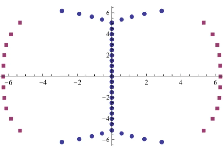
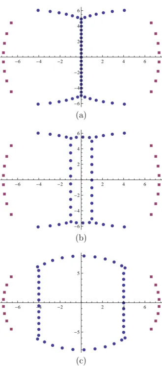
zk+1 =zk+ 1, k = 1, . . . , ℓ−1, (3.64) where ℓ is called the length of the string. It is obvious from (3.62) that neither of the polynomials A±(z) could have exact strings of the length greater then two. Indeed, the only such zeroes can be atz =±¹₂, thusA±(z) might only have (possibly multiple) 2-strings at z = ±¹₂. The same analysis extends to the zero-field case as well. Note, in particular, that the long strings on the imaginary axis of the variableu=iz, shown in fig. 1 in section 4.5, are not exact.

4 Removing the Twist: The φ → 0 Limit

In the previous chapter 3 we have used a regulator φ to obtain finite quantities when taking traces over infinite dimensional oscillator spaces. It is interesting that this natural quantity φ corresponds precisely to the spin chain with magnetic flux discussed in the review chapter 2. In the present chapter we will deal with the operation of taking this regulating flux away. This involves a significant symmetry enhancement to a global SU(2) symmetry of the spectrum of the Heisenberg chain, “weakly” broken by the twist. Moreover we would like to make contact with the results of [18], see also the attempt in [27], as well as the findings in [28]. It is interesting to explicitly work out the operatorsQ± for small spin chain lengths L. This is done in appendix B. In line with their construction, the operators