The Zero Emissions Commitment Model Intercomparison Project (ZECMIP) contribution to C4MIP: quantifying committed climate changes following zero carbon emissions

(1)

https://doi.org/10.5194/gmd-12-4375-2019

The Zero Emissions Commitment Model Intercomparison Project (ZECMIP) contribution to C4MIP: quantifying committed climate changes following zero carbon emissions

Chris D. Jones¹, Thomas L. Frölicher^2,3, Charles Koven⁴, Andrew H. MacDougall⁵, H. Damon Matthews⁶, Kirsten Zickfeld⁷, Joeri Rogelj^8,9, Katarzyna B. Tokarska^10,11, Nathan P. Gillett¹², Tatiana Ilyina¹³, Malte Meinshausen^14,15, Nadine Mengis^7,16, Roland Séférian¹⁷, Michael Eby¹⁸, and Friedrich A. Burger^2,3

1Met Office Hadley Centre, Exeter, EX1 3PB, UK

2Climate and Environmental Physics, Physics Institute, University of Bern, Bern, 3012, Switzerland

3Oeschger Centre for Climate Change Research, University of Bern, Bern, 3012, Switzerland

4Climate and Ecosystem Sciences Division, Lawrence Berkeley National Laboratory, Berkeley, CA 94720, USA

5St. Francis Xavier University, Antigonish, B2G 2W5, Canada

6Concordia University, Montreal, Quebec, H3G 1M8, Canada

7Department of Geography, Simon Fraser University, Burnaby, V5A 1S6, Canada

8International Institute for Applied Systems Analysis (IIASA), 2361 Laxenburg, Austria

9Grantham Institute for Climate Change and the Environment, Imperial College London, London, SW7 2AZ, UK

10School of Geosciences, The University of Edinburgh, Edinburgh, EH9 3FF, UK

11Institute for Atmospheric and Climate Science, ETH Zurich, Zurich, Switzerland

12Canadian Centre for Climate Modelling and Analysis, Environment and Climate Change Canada, Victoria, BC, V8W 2Y2, Canada

13Max Planck Institute for Meteorology, Bundesstraße 53, 20146 Hamburg, Germany

14Climate & Energy College, School of Earth Sciences, The University of Melbourne, Parkville 3010, Victoria, Australia

15Potsdam Institute for Climate Impact Research (PIK), Telegrafenberg, 14412 Potsdam, Germany

16Helmholtz Centre for Ocean Research Kiel (GEOMAR), Düsternbrooker Weg 20, 24105 Kiel, Germany

17Centre National de Recherches Météorologiques (CNRM), Université de Toulouse, Météo-France, CNRS, Toulouse, France

18School of Earth and Ocean Sciences, University of Victoria, Victoria, BC, V8W 2Y2, Canada Correspondence:Chris D. Jones (chris.d.jones@metoffice.gov.uk)

Received: 25 May 2019 – Discussion started: 28 June 2019

Revised: 6 September 2019 – Accepted: 11 September 2019 – Published: 15 October 2019

Abstract. The amount of additional future temperature change following a complete cessation of CO₂emissions is a measure of the unrealized warming to which we are committed due to CO2already emitted to the atmosphere. This

“zero emissions commitment” (ZEC) is also an important quantity when estimating the remaining carbon budget – a limit on the total amount of CO2emissions consistent with limiting global mean temperature at a particular level. In the recent IPCC Special Report on Global Warming of 1.5^◦C, the carbon budget framework used to calculate the remaining carbon budget for 1.5^◦C included the assumption that the ZEC due to CO₂emissions is negligible and close to zero.

Previous research has shown significant uncertainty even in the sign of the ZEC. To close this knowledge gap, we pro- pose the Zero Emissions Commitment Model Intercompar- ison Project (ZECMIP), which will quantify the amount of unrealized temperature change that occurs after CO2 emissions cease and investigate the geophysical drivers behind this climate response. Quantitative information on ZEC is a key gap in our knowledge, and one that will not be addressed by currently planned CMIP6 simulations, yet it is crucial for verifying whether carbon budgets need to be adjusted to ac- count for any unrealized temperature change resulting from past CO₂emissions. We request only one top-priority sim-

(2)

ulation from comprehensive general circulation Earth system models (ESMs) and Earth system models of intermediate complexity (EMICs) – a branch from the 1 % CO₂run with CO₂emissions set to zero at the point of 1000 PgC of total CO₂ emissions in the simulation – with the possibil- ity for additional simulations, if resources allow. ZECMIP is part of CMIP6, under joint sponsorship by C4MIP and CDR- MIP, with associated experiment names to enable data sub- missions to the Earth System Grid Federation. All data will be published and made freely available.

1 Introduction

The zero emissions commitment (ZEC), or the amount of global mean temperature change that is still expected to oc- cur after a complete cessation of CO₂ emissions, is a key component of estimating the remaining carbon budget to stay within global warming targets as well as an important met- ric to understand impacts and reversibility of climate change (Matthews and Solomon, 2013). Much effort is put into mea- suring and constraining the TCRE – the Transient Climate Response to cumulative CO₂Emissions (Allen et al., 2009;

Matthews et al., 2009; Zickfeld et al., 2009; Raupach et al., 2011; Gillett et al., 2013; Tachiiri et al., 2015; Goodwin et al., 2015; Steinacher and Joos, 2016; MacDougall, 2016; Ehlert et al., 2017; Millar and Friedlingstein, 2018). The TCRE de- scribes the ratio between CO2-induced warming and cumulative CO2emissions up to the same point in time, but it does not capture any delayed warming response to CO2emissions beyond the point that emissions reach zero. When using the TCRE to derive the carbon budget consistent with a specific temperature limit, the ZEC is often assumed to be negligible and close to zero (Matthews et al., 2017; Rogelj et al., 2011, 2018). Constraints on ZEC have not been systematically re- searched so far, although both TCRE and ZEC are required to relate carbon emissions to the eventual equilibrium warming (Rogelj et al., 2018).

It has been shown that continued CO₂ removal by natural sinks following cessation of emissions offsets the continued warming that would result from stabilized CO2con- centration (Matthews and Caldeira, 2008; Solomon et al., 2009; Frölicher and Joos, 2010; Matthews and Weaver, 2010;

Joos et al., 2013). This is partly due to the ocean uptake of both heat and carbon sharing some similar processes and timescales, and it is therefore expected to lead to ZEC being small (Allen et al., 2018; Ehlert and Zickfeld, 2017; Gillett et al., 2011; Matthews and Zickfeld, 2012). This has been shown to be a general result across a range of models (Gillett et al., 2011; Lowe et al., 2009; Matthews and Zickfeld, 2012;

Zickfeld et al., 2013). Most such literature focused on long timescales (up to and beyond a century). This led IPCC SR15 (Rogelj et al., 2018) to make the assumption for the esti- mation of carbon budgets that for timescales up to a cen-

tury ZEC was uncertain, yet centred around zero. More detailed studies, however, have shown that ZEC can be (a) non- zero, possibly of either positive or negative sign that may change in time during the period following emissions ceasing (Frölicher et al., 2014; Frölicher and Paynter, 2015), and (b) it is both state and rate dependent – i.e. it varies depending on the amount of carbon emitted and taken up by the natural carbon sinks, and the CO₂ emissions pathway of its emissions prior to cessation (Ehlert and Zickfeld, 2017; Krasting et al., 2014; MacDougall, 2019).

When we consider stringent climate targets, such as limiting global mean warming to 1.5 or 2^◦C, and in light of approximately 1^◦C warming to date and potential future warming from non-CO2greenhouse gases, an uncertainty in ZEC of 0±0.1^◦C already leads to a substantial uncertainty in the remaining carbon budget. Given the current central estimate of the TCRE of 1.6^◦C per 1000 PgC (Collins et al., 2013), each 0.1^◦C of warming equates to approximately 60 PgC of CO₂ emissions, or approximately 6 years of current fossil fuel emission rates (Le Quéré et al., 2018). It has therefore emerged that quantitative information on ZEC is a key gap in our knowledge, and one that is not filled by currently planned simulations for the sixth phase of the Coupled Model Inter- comparison Project (CMIP6).

ZECMIP aims to fill this gap as efficiently as possible.

Thereby, ZECMIP will support the assessment of remaining carbon budgets based on the CMIP6 simulations and super- sede the current practice of applying a single model estimate of ZEC or an estimate from a limited number of studies from the literature. Much more preferable is to coordinate par- allel studies, with Earth system general circulation models (ESMs) and Earth system models of intermediate complexity (EMICs), to measure both TCRE and ZEC in a common scenario. Hence, we proposed using the 1 % per annum increase in CO₂concentration experiment (1pctCO2) from the CMIP6 Diagnostic Evaluation and Characterization of Klima (DECK) simulations (Eyring et al., 2016) as a common baseline simulation for estimating both the TCRE and the ZEC.

As a late addition to CMIP6, ZECMIP has been designed to address this important question with only one high-priority simulation – A1: “a zero-emission experiment following 1000 PgC emissions” – implemented as a branching off from the 1pctCO2 simulation from the point at which 1000 PgC in diagnosed cumulative emissions is reached. Additional simulations of lower priority are also suggested, which will aid further analysis. Branching from this idealized simulation avoids complications of non-CO₂forcing and land-use or nitrogen deposition impacts on the carbon cycle, and also makes the quantified ZEC consistent with the TCRE values also derived from this simulation.

This paper documents the ZECMIP simulations with a fo- cus on the details needed for ESMs and EMICs to contribute the top-priority simulation of a ZEC run from the point of 1000 PgC emissions following 1 % per year growth in CO₂.

(3)

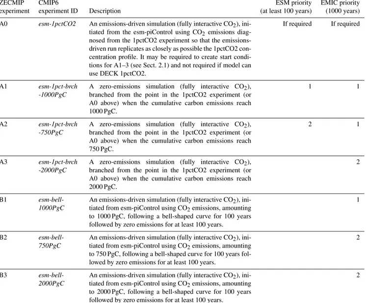
Table 1.ZECMIP simulations and priorities for ESMs and EMICs.

ZECMIP CMIP6 ESM priority EMIC priority

experiment experiment ID Description (at least 100 years) (1000 years)

A0 esm-1pctCO2 An emissions-driven simulation (fully interactive CO₂), initiated from the esm-piControl using CO₂emissions diagnosed from the 1pctCO2 experiment so that the emissions- driven run replicates as closely as possible the 1pctCO2 concentration profile. It may be required to create start conditions for A1–3 (see Sect. 2.1) and not required if model can use DECK 1pctCO2.

If required If required

A1 esm-1pct-brch

-1000PgC

A zero-emissions simulation (fully interactive CO₂), branched from the point in the 1pctCO2 experiment (or A0 above) when the cumulative carbon emissions reach 1000 PgC.

1 1

A2 esm-1pct-brch

-750PgC

2 1

A3 esm-1pct-brch

-2000PgC

2

B1 esm-bell-

1000PgC

An emissions-driven simulation (fully interactive CO₂), initiated from esm-piControl using CO₂emissions, amounting to 1000 PgC, following a bell-shaped curve for 100 years followed by zero emissions for at least 100 years.

1

B2 esm-bell-

750PgC

An emissions-driven simulation (fully interactive CO₂), initiated from esm-piControl using CO₂emissions, amounting to 750 PgC, following a bell-shaped curve for 100 years followed by zero emissions for at least 100 years.

2

B3 esm-bell-

2000PgC

An emissions-driven simulation (fully interactive CO₂), initiated from esm-piControl using CO₂emissions, amounting to 2000 PgC, following a bell-shaped curve for 100 years followed by zero emissions for at least 100 years.

2

ZECMIP analysis will draw on carbon cycle feedbacks and process understanding from C4MIP (Coupled Climate Carbon Cycle Model Intercomparison Project; Jones et al., 2016) and aims to complement analysis on reversibility and CO₂ removal under CDRMIP (Carbon Dioxide Re- moval Model Intercomparison Project; Keller et al., 2018).

Both C4MIP and CDRMIP encourage participation in the ZECMIP top-priority simulation. For simplicity, the data request is a replica of that for the CMIP6 emission-driven historical simulation (esm-hist). No new variables have been added. For EMICs the request is to output the same model variables as from the 1 % run, which forms the basis of ZECMIP, with the one addition of also providing atmospheric CO2 concentration. Data can be published via the Earth System Grid Federation (ESGF) (for ESMs contribut- ing to CMIP6). An equivalent data repository will be avail-

able for EMICs and likely based at the University of Victo- ria – details will be communicated during summer 2019 via C4MIP and CDRMIP websites.

2 Simulation protocol

Due to time pressures and a limit to computational resources for modelling groups, ZECMIP has just one high-priority simulation, with a second lower-priority simulation suggested (See Table 1). Other lower-priority simulations are also detailed and welcomed. For EMIC model groups, there is an extended protocol with longer and additional experiments. We welcome ESM groups to also perform these additional simulations, but this is not required. Given that the overall CMIP6 protocol (Eyring et al., 2016) has been years in development, it is not possible to initiate a new MIP nor

(4)

allocate new CMIP tier-1 simulations during 2019. Instead, ZECMIP simulations are being included under C4MIP and CDRMIP and included in CMIP as tier-2 and tier-3 simulations so that they do not become mandatory “entry card” re- quirements for C4MIP or CDRMIP. Hence, our top-priority simulation, A1, is classed as a CMIP tier-2 simulation; all others are classified as tier-3 simulations. However, Table 1 lists the simulations prioritized by ZECMIP to guide groups who have limited resources to perform the simulations. We hope as many groups as possible perform as many of the simulations as possible, and participating model groups will be offered co-authorship on the article containing the analysis to be submitted this year (by December 2019).

2.1 Simulation set A: abrupt zero emissions

All ZECMIP simulations are required to be in “emissions- driven mode”. Experiments under set A require branching off from a simulation where CO₂concentration follows a 1 % per annum increase from pre-industrial levels. This presents model groups with a choice of how to initialize experiments A1 to A3. Some models may have the capability to switch from concentration-driven to emissions-driven con- figurations but some models may not or model groups may not have confidence that they can do so without a shock to the model system. In the case of the former, the concentration- driven DECK 1pctCO2 simulation can be used to initiate experiments A1 to A3. Otherwise, models should perform simulation A0 to generate initial conditions for A1 to A3.

We do not specify a precise definition of how to make this choice but suggest that when an emissions-driven control run is initiated from a concentration-driven control run, any subsequent change in atmospheric CO₂, major carbon stores, or global temperature should all be approximately within the expected interannual variability of the control run. We note that if simulation A0 is required to initialize the A1 simulation, then it should be treated as equal priority to A1 and data submission to the ESGF is required.

A0: “esm-1pctCO2”.Run an emissions-driven version of 1pctCO2 to get to the branch-off point for A1 to A3. The requirement to run this is a model-by-model decision. The compatible emissions time series for this simulation should be calculated from the 1pctCO2 and used to branch esm- 1pctCO2 from esm-piControl to replicate the 1 % profile as closely as possible up to the desired cumulative emission before setting emissions to zero from this point.

The compatible emission rateE(PgC yr⁻¹)can be calculated from the 1pctCO2 concentration-driven simulation, as described in Jones et al. (2013; see their Sect. 2b). In sum- mary, changes in atmospheric CO₂concentration (C_A)are balanced by anthropogenic emissions,E, and changes in the natural land and ocean carbon reservoirs (C_LandC_O, respectively). Therefore, the compatible emissions can be calcu-

lated simply as E= d

dt(CTot)= d

dt(CA)+ d

dt(CL+CO),

where units of all quantities are in petagrams of carbon (PgC). Changes in atmospheric CO₂can be converted from concentration (ppm) to mass (PgC) by a simple scaling of 2.12. Typically, the time derivative,d/dt, is taken to imply changes per year – i.e. annual changes in the carbon stores are used in order to calculate annual emission,E. The calcu- lation is done using global total amounts. Emissions should be prescribed as globally uniform at the surface. Models that have run multiple ensemble members for the concentration- driven 1pctCO2 experiment should use ensemble-mean values ofC_LandC_Ofrom those runs to derive the emissions for forcing the esm-1pctCO2 simulation. This will minimize the effect of interannual variability of carbon sinks on the diagnosed compatible emissions. If desired, numerical smoothing of the global mean time series of emissions may also be applied as long as the cumulative total is not affected.

ZECMIP simulation set A is based on CO₂-only 1 % run (either concentration-driven DECK “1pctCO2” or the above described A.0 “esm-1pctCO2”), with all the other external forcing held at pre-industrial conditions (i.e. non-CO2green- house gases, aerosols, volcanoes, land-use changes, solar ir- radiance). After following the CO2concentration up to the level described below, branch off with prognostic CO2(a.k.a.

“emissions driven”) but with carbon emissions set to zero (E=0). Simulate the subsequent reduction in atmospheric CO₂and change in climate for at least 100 years.

Branch off at the following given cumulative emissions.

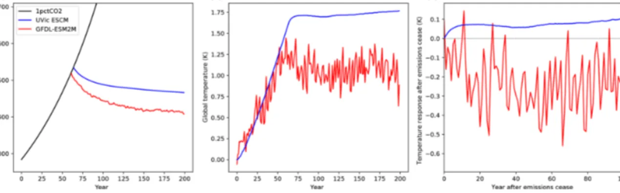
– A1: “esm-1pct-brch-1000PgC”, 1000 PgC. This is the ZECMIP top-priority simulation. This corresponds to approximately 2^◦C CO2-induced warming above pre- industrial levels (with the year 1850 here taken as proxy for pre-industrial levels). Figure 1 shows example results from two models.

– A2: “esm-1pct-brch-750PgC”, 750 PgC. This is a simulation corresponding to approximately 1.5^◦C CO2- induced warming above 1850 and is optional.

– A3: “esm-1pct-brch-2000PgC”, 2000 PgC. This simulation will give insights into ZEC for a possible higher CO₂-induced warming and is optional.

The experimental design is for all models to branch off at a common cumulative carbon emission level, acknowledging that this will mean a different year for ceasing emissions and thus a slightly different atmospheric CO₂concentration and departure of global mean temperature from 1850 for each model at the beginning of the ZECMIP simulations. EMICs should run the simulations for at least 1000 years. We antici- pate that the small signal-to-noise ratio of the ZEC versus the internal climate variability may require an ensemble of simulations. However, acknowledging ESM time pressure and

(5)

Figure 1.Example results from simulation A1 from the UVic ESCM (Weaver et al., 2001; MacDougall and Knutti, 2016; blue) and GFDL- ESM2M (Dunne et al., 2012, 2013; red) models.(a)CO₂concentration prescribed (black line) in the 1pctCO2 simulation and simulated (red, blue lines) by the two models;(b)simulated global mean surface air temperature for the same period;(c)global mean temperature response from the branch point off the 1 % simulation with zero subsequent emissions.

Figure 2. Time series of global CO₂ emissions for bell-shaped curve pathways B1 to B3. The numbers in the legend indicate the cumulative amount of CO₂emissions for each simulation.

limits to computational resources, only one ensemble mem- ber is required.

Experiment A1 aims to quantify ZEC at 1000 PgC (cumulative emissions) at which point TCRE will be calculated.

A2 and A3 explore thestatedependence of ZEC at approximately 1.5^◦C CO₂-induced warming above 1850 and at sig- nificantly higher cumulative emissions, respectively.

2.2 Simulation set B: bell-shaped zero emissions This second set of experiments, B1 to B3, aims to explore the dependence of ZEC on CO₂emissions rateby following a pathway emitting the same cumulative emissions as A1 to A3 but with a smooth transition to zero emissions, followed by 100 years ofE=0 (EMICs for at least 1000 years).

The main purpose of this experiment is to quantify the dependency of ZEC on emission pathways and the emission rate prior to the point when TCRE is evaluated as the Earth system is subject to comparatively low emissions, occurring

just before the TCRE evaluation point of zero emissions after 100 years of simulation – compared to the sudden cessation of high emissions in experiments A1, A2, and A3.

The conventional way of estimating TCRE is using 1 % CO2 model simulations. The tier-1 A1 simulation thus pro- vides the most complementary and internally consistent quantification of the ZEC, which is why we consider this to be the top priority. However, additional ZECMIP experiments with more gradually phased out emissions enable us to determine how the ZEC is expected to materialize over the timescales of more societally relevant CO₂emissions reduction rates. Analysis of pairs of A and B experiments will allow us to generalize the findings for other emission reduction pathways, allowing us to answer the question of whether temperature will continue to increase following a more real- istic cessation of CO₂emissions.

These B experiments are run in emissions-driven config- uration (CO₂-only: following 1pctCO2 and piControl, all other external forcing is fixed at pre-industrial levels), as- suming a bell-shaped emissions profile (Fig. 2), for which we have chosen an arbitrary Gaussian distribution (see Ap- pendix A). At the end of 100 years emissions profile, simulations should continue with zero emissions for at least 100 years (for ESMs) or 1000 years (EMICs).

The bell-shaped curve is designed to give the following cumulative emissions.

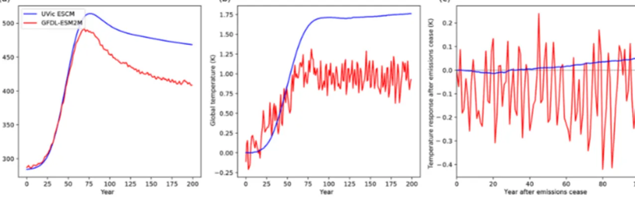
– B1: “esm-bell-1000PgC”, 1000 PgC (Fig. 3 shows example results from two models);

– B2: “esm-bell-750PgC”, 750 PgC;

– B3: “esm-bell-2000PgC”, 2000 PgC.

By design, this set B utilizes the same cumulative emissions as the respective simulations in set A experience up to their branch point. These emissions are applied over 100 years, followed by zero emissions for 100 years (ESMs)

(6)

Figure 3.Example results from simulation B1 from the UVic ESCM (Weaver et al., 2001; MacDougall and Knutti, 2016; blue) and GFDL- ESM2M (Dunne et al., 2012, 2013; red) models.(a)CO₂concentration simulated by the two models;(b)simulated global mean surface air temperature for the same period;(c)global mean temperature response from year 100 onwards with zero subsequent emissions.

or 1000 years (EMICs). These additional simulations allow for a direct comparison of the two ZEC experiment sets, given the same amount of cumulative emissions. A model decision is required on the spatial pattern of emissions – we suggest globally uniform at surface. The time series of global CO₂ emissions for the above curves is listed in Appendix A and is hosted on the C4MIP (http:

//www.c4mip.net/index.php?id=3387, last access: 6 Septem- ber 2019) and CDRMIP (https://www.kiel-earth-institute.de/

CDR_Model_Intercomparison_Project.html, last access: 6 September 2019) websites.

3 ZECMIP outlook and conclusions

The experiments outlined above will lay the foundation for coordinated multi-model analysis of the zero emissions commitment. The absence of a dedicated experiment to quantify ZEC across CMIP models was identified and is addressed by our top-priority experiment, A1. Investigations into the state, rate, and pathway dependence of the ZEC are aided by further experiments with sudden and gradual cessation of emissions. ZECMIP was motivated to keep the experiment design both lightweight and simple to follow; in future, further simulations could be defined to explore additional is- sues such as cessation of emissions of non-CO2greenhouse gases, aerosols, or from land-use activities. The complexity of defining such experiments precluded an exhaustive inclu- sion in this first generation of ZECMIP but we acknowledge the importance of rate and pathway dependency, as well non- CO₂aspects in determining ZEC and the remaining carbon budget overall (MacDougall et al., 2015; Rogelj et al., 2015;

Mengis et al., 2018; Tokarska et al., 2018).

The requirement for specific information regarding ZEC to assess remaining carbon budgets was identified in the IPCC Special Report on Global Warming of 1.5^◦C (Rogelj et al., 2018). An initial paper exploring ZEC in this context, explic- itly on timescales of relevance to 21st century carbon budgets, is planned on a timeline that could support an improved

assessment of the ZEC and its influence on carbon budgets in the IPCC Sixth Assessment Report. All participating model groups who are able to complete and provide data for simulation A1 in time will be invited to join this analysis.

ZECMIP welcomes community engagement in the participation of simulations and their analysis, as well as input to future analysis and experimental design. We hope to bring to- gether ESMs and EMICs to enable analysis across timescales from decadal through centennial to millennial.

Furthermore, as a set of numerical simulations, ZECMIP is intended to complement existing CMIP activity, especially on carbon cycle feedbacks, CO2removal, and reversibility of the climate system. C4MIP simulations aim to address model evaluation during the historical period from 1850 to present day, along with process-level feedback analysis. CDRMIP adds to this with exploration of the processes controlling the response of the climate and carbon cycle to negative emissions and reversibility of components of the Earth system.

ZECMIP will contribute additional simulations and analysis to aid understanding of the mechanisms of the climate response to CO₂emissions and relationships between transient and equilibrium climate sensitivities. We hope that ZECMIP analysis will address the crucial knowledge gap surrounding committed warming following ceasing emissions and will provide valuable support for assessment of carbon budgets to achieve climate targets.

Data availability. As with all CMIP6-endorsed MIPs, the model output from the ZECMIP simulations described in this paper will be distributed through the Earth System Grid Federation (ESGF) with version control and digital object identifiers (DOIs) assigned. No additional model forcings are required beyond those already used for piControl and 1pctCO2 simulations apart from the emission in- puts for the proposed B experiments, which are described in Ap- pendix A of this paper and are hosted on the C4MIP and CDRMIP websites.

(7)

Appendix A: CO₂emissions for bell-shaped curve simulations B1–3

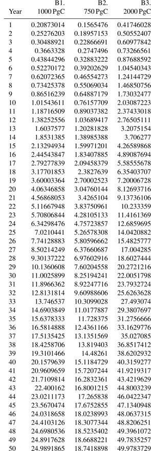
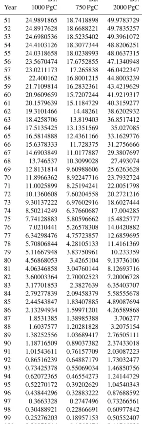
This table lists the global CO₂emissions (PgC yr⁻¹) to be applied for the first 100 years of simulations B1–3. This period should be followed by at least 100 years of zero emissions for ESMs or 1000 years for EMICs (see Fig. 2). These emissions should be prescribed as globally uniform at the surface.

The data were calculated from a Gaussian curve according to

E=k 1

√

2π σ²e⁻

(x−µ)2 2σ2 ,

where emissions,E, are scaled by a constant,k, so that the cumulative total matches the required amount for each scenario (1000 PgC for B1, 750 PgC for B2, 2000 PgC for B3).

The parameters were set asµ=50 as the centre of the 100- year period and σ=100/6 so that the distribution spans 3 standard deviations about the centre.

These data in .csv file format are available from the C4MIP (http://www.c4mip.net/index.php?id=3387, last access: 6 September 2019) and CDRMIP (https://www.kiel-earth-institute.de/CDR_Model_

Intercomparison_Project.html, last access: 6 September 2019) websites.

Table A1.Global CO₂emissions (PgC yr⁻¹) to be applied during each year for the first 100 years of simulations B1–3.

B1. B2. B3.

Year 1000 PgC 750 PgC 2000 PgC 1 0.20873014 0.1565476 0.41746028 2 0.25276203 0.18957153 0.50552407 3 0.30488921 0.22866691 0.60977842 4 0.3663328 0.2747496 0.73266561 5 0.43844296 0.32883222 0.87688592 6 0.52270172 0.39202629 1.04540343 7 0.62072365 0.46554273 1.24144729 8 0.73425378 0.55069034 1.46850756 9 0.86516239 0.64887179 1.73032477 10 1.01543611 0.76157709 2.03087223 11 1.18716509 0.89037382 2.37433018 12 1.38252556 1.03689417 2.76505111 13 1.6037577 1.20281828 3.2075154 14 1.8531385 1.38985388 3.706277 15 2.13294934 1.59971201 4.26589868 16 2.44543847 1.83407885 4.89087694 17 2.79277839 2.09458379 5.58555678 18 3.17701853 2.3827639 6.35403707 19 3.60003364 2.70002523 7.20006728 20 4.06346858 3.04760144 8.12693716 21 4.56868053 3.4265104 9.13736106 22 5.11667948 3.83750961 10.233359 23 5.70806844 4.28105133 11.4161369 24 6.34298476 4.75723857 12.6859695 25 7.0210441 5.26578308 14.0420882 26 7.74128883 5.80596662 15.4825777 27 8.50214249 6.37660687 17.004285 28 9.30137222 6.97602916 18.6027444 29 10.1360608 7.60204558 20.2721216 30 11.0025899 8.25194241 22.0051798 31 11.8966362 8.92247716 23.7932724 32 12.8131814 9.60988606 25.6263628 33 13.746537 10.3099028 27.493074 34 14.6903849 11.0177887 29.3807697 35 15.6378333 11.728375 31.2756666 36 16.5814888 12.4361166 33.1629776 37 17.5135425 13.1351569 35.027085 38 18.4258706 13.819403 36.8517412 39 19.3101466 14.48261 38.6202932 40 20.1579639 15.1184729 40.3159277 41 20.9609659 15.7207244 41.9219317 42 21.7109814 16.2832361 43.4219629 43 22.400162 16.8001215 44.8003239 44 23.0211173 17.265838 46.0422347 45 23.5670474 17.6752855 47.1340948 46 24.0318658 18.0238993 48.0637315 47 24.4103126 18.3077344 48.8206251 48 24.6980536 18.5235402 49.3961072 49 24.8917628 18.6688221 49.7835257 50 24.9891865 18.7418898 49.9783729

(8)

Table A1.Continued.

B1. B2. B3.

Year 1000 PgC 750 PgC 2000 PgC 51 24.9891865 18.7418898 49.9783729 52 24.8917628 18.6688221 49.7835257 53 24.6980536 18.5235402 49.3961072 54 24.4103126 18.3077344 48.8206251 55 24.0318658 18.0238993 48.0637315 56 23.5670474 17.6752855 47.1340948 57 23.0211173 17.265838 46.0422347 58 22.400162 16.8001215 44.8003239 59 21.7109814 16.2832361 43.4219629 60 20.9609659 15.7207244 41.9219317 61 20.1579639 15.1184729 40.3159277 62 19.3101466 14.48261 38.6202932 63 18.4258706 13.819403 36.8517412 64 17.5135425 13.1351569 35.027085 65 16.5814888 12.4361166 33.1629776 66 15.6378333 11.728375 31.2756666 67 14.6903849 11.0177887 29.3807697 68 13.746537 10.3099028 27.493074 69 12.8131814 9.60988606 25.6263628 70 11.8966362 8.92247716 23.7932724 71 11.0025899 8.25194241 22.0051798 72 10.1360608 7.60204558 20.2721216 73 9.30137222 6.97602916 18.6027444 74 8.50214249 6.37660687 17.004285 75 7.74128883 5.80596662 15.4825777 76 7.0210441 5.26578308 14.0420882 77 6.34298476 4.75723857 12.6859695 78 5.70806844 4.28105133 11.4161369 79 5.11667948 3.83750961 10.233359 80 4.56868053 3.4265104 9.13736106 81 4.06346858 3.04760144 8.12693716 82 3.60003364 2.70002523 7.20006728 83 3.17701853 2.3827639 6.35403707 84 2.79277839 2.09458379 5.58555678 85 2.44543847 1.83407885 4.89087694 86 2.13294934 1.59971201 4.26589868 87 1.8531385 1.38985388 3.706277 88 1.6037577 1.20281828 3.2075154 89 1.38252556 1.03689417 2.76505111 90 1.18716509 0.89037382 2.37433018 91 1.01543611 0.76157709 2.03087223 92 0.86516239 0.64887179 1.73032477 93 0.73425378 0.55069034 1.46850756 94 0.62072365 0.46554273 1.24144729 95 0.52270172 0.39202629 1.04540343 96 0.43844296 0.32883222 0.87688592 97 0.3663328 0.2747496 0.73266561 98 0.30488921 0.22866691 0.60977842 99 0.25276203 0.18957153 0.50552407 100 0.20873014 0.1565476 0.41746028

(9)

Author contributions. CDJ, TLF, CK, AHM, HDM, KZ, JR, KBT, NPG, TI, MM, NM, and RS participated in workshop discussions to identify research needs towards better understanding of remaining carbon budgets. ZECMIP was the direct outcome of this workshop and the participants were all active in breakout discussions to design the experimental protocol described here. ME was instrumen- tal in providing support and data storage for EMIC simulations and provided valuable guidance around the data request detailed in the article. FAB performed simulations with GFDL-ESM2M to specifi- cally test the experimental design and provide data for Figs. 1 and 3.

All authors contributed to the development of the article, provided text, and responded to review comments and revisions.

Competing interests. The authors declare that they have no conflict of interest.

Acknowledgements. This protocol was devised at a Global Carbon Project workshop supported by H2020 EU project CRESCENDO under grant agreement no. 641816. Chris D. Jones was supported by the Joint UK BEIS/Defra Met Office Hadley Centre Climate Pro- gramme (GA01101). Joeri Rogelj, Katarzyna Tokarska and Roland Séférian were supported by H2020 EU project CONSTRAIN under grant agreement no. 820829. Tatiana Ilyina and Thomas L.

Frölicher were supported by H2020 EU project CCICC under grant agreement no. 821003. Thomas L. Frölicher acknowledges support from the Swiss National Science Foundation under grant PP00P2_170687. GFDL-ESM2M simulations were performed at the Swiss National Supercomputing Centre (CSCS). Kirsten Zick- feld and Andrew H. MacDougall acknowledge support from the National Sciences and Engineering Research Council of Canada’s Discovery Grants Program. Charles Koven acknowledges support from the US DOE BER Regional & Global Model Analysis pro- gramme through the Early Career Research Program and the RU- BISCO SFA projects. Katarzyna B. Tokarska was also supported by the UK NERC-funded SMURPHs project (NE/N006143/1).

Financial support. This research has been supported by the Euro- pean Commission (grant no. CRESCENDO (641816)).

Review statement. This paper was edited by Carlos Sierra and re- viewed by two anonymous referees.

References

Allen, M. R., Frame, D. J., Huntingford, C., Jones, C. D., Lowe, J.

A., Meinshausen, M., and Meinshausen, N.: Warming caused by cumulative carbon emissions towards the trillionth tonne, Nature, 458, 1163–1166, https://doi.org/10.1038/nature08019, 2009.

Allen, M. R., Dube, O. P., Solecki, W., Aragón-Durand, F., Cramer, W., Humphreys, S., Kainuma, M., Kala, J., Mahowald, N., Mu- lugetta, Y., Perez, R., Wairiu, M., and Zickfeld, K.: Chapter 1 Framing and Context, in: Global warming of 1.5^◦C, An IPCC Special Report on the impacts of global warming of 1.5^◦C above

pre-industrial levels and related global greenhouse gas emission pathways, in the context of strengthening the global response to the threat of climate change, World Meteorological Organization, Geneva, Switzerland, 2018.

Collins, M., Knutti, R., Arblaster, J., Dufresne, J.-L., Fichefet, T., Friedlingstein, P., Gao, X., Gutowski, W. J., Johns, T., Krinner, G., Shongwe, M., Tebaldi, C., Weaver, A. J., and Wehner, M.:

Long-term Climate Change: Projections, Commitments and Irre- versibility, in: Climate Change 2013: The Physical Science Ba- sis. Contribution of Working Group I to the Fifth Assessment Re- port of the Intergovernmental Panel on Climate Change, edited by: Stocker, T. F., Qin, D., Plattner, G.-K., Tignor, M., Allen, S.

K., Boschung, J., Nauels, A., Xia, Y., Bex, V., and Midgley, P.

M., Cambridge University Press, Cambridge, United Kingdom and New York, NY, USA, 2013.

Dunne, J. P., John, J. G., Adcroft, A. J., Griffies, S. M., Hallberg, R.

W., Shevliakova, E. N., Stouffer, R. J., Cooke, W., Dunne, K. A., Harrison, M. J., Krasting, J. P., Levy, H., Malyshev, S. L., Milly, P. C. D., Phillipps, P. J., Sentman, L. T., Samuels, B. L., Spelman, M. J., Winton, M., Wittenberg, A. T., and Zadeh, N.: GFDL’s ESM2 global coupled climate-carbon Earth System Models Part I: Physical formulation and baseline simulation characteristics, J. Climate, 25, 6646–6665, https://doi.org/10.1175/JCLI-D-11- 00560.1, 2012.

Dunne, J. P., John, J. G., Shevliakova, E., Stouffer, R. J., Krasting, J. P., Malyshev, S. L., Milly, P. C. D., Sentman, L. T., Adcroft, A. J., Cooke, W., Dunne, K. A., Griffies, S. M., Hallberg, R.

W., Harrison, M. J., Levy, H., Wittenberg, A. T., Phillips, P. J., and Zadeh, N.: GFDL’s ESM2 Global Coupled Climate–Carbon Earth System Models. Part II: Carbon System Formulation and Baseline Simulation Characteristics, J. Climae, 26, 2247–2267, https://doi.org/10.1175/JCLI-D-12-00150.1, 2013.

Ehlert, D. and Zickfeld, K.: What determines the warming commitment after cessation of CO₂emissions?, Environ. Res. Lett., 12, 015002, https://doi.org/10.1088/1748-9326/aa564a, 2017.

Ehlert, D., Zickfeld, K., Eby, M., and Gillett, N.: The sensitivity of the proportionality between temperature change and cumulative CO₂emissions to ocean mixing, J. Climate, 30, 2921–2935, https://doi.org/10.1175/JCLI-D-16-0247.1, 2017.

Eyring, V., Bony, S., Meehl, G. A., Senior, C. A., Stevens, B., Stouffer, R. J., and Taylor, K. E.: Overview of the Coupled Model Intercomparison Project Phase 6 (CMIP6) experimental design and organization, Geosci. Model Dev., 9, 1937–1958, https://doi.org/10.5194/gmd-9-1937-2016, 2016

Frölicher, T. L. and Joos, F.: Reversible and irreversible impacts of greenhouse gas emissions in multi-century projections with the NCAR global coupled carbon cycle-climate model, Clim. Dy- nam., 35, 1439–1459, https://doi.org/10.1007/s00382-009-0727- 0, 2010.

Frölicher, T. L. and Paynter, D. J.: Extending the relationship between global warming and cumulative carbon emissions to multi-millennial timescales, Environ. Res. Lett., 10, 075002, https://doi.org/10.1088/1748-9326/10/7/075002, 2015.

Frölicher, T. L., Winton, M., and Sarmiento, J. L.: Continued global warming after CO₂emissions stoppage, Nat. Clim. Change, 4, 40–44, https://doi.org/10.1038/nclimate2060, 2014.

Gillett, N. P., Arora, V. K., Zickfeld, K., Marshall, S. J., and Mer- ryfield, W. J.: Ongoing climate change following a complete

(10)

cessation of carbon dioxide emissions, Nat. Geosci., 4, 83–87, https://doi.org/10.1038/ngeo1047, 2011.

Gillett, N. P., Arora, V. K., Matthews, D., and Allen, M. R.: Con- straining the ratio of global warming to cumulative CO₂emissions using CMIP5 simulations, J. Climate, 26, 6844–6858, https://doi.org/10.1175/JCLI-D-12-00476.1, 2013.

Goodwin, P., Williams, R. G., and Ridgwell, A.: Sensitivity of climate to cumulative carbon emissions due to compensation of ocean heat and carbon uptake, Nat. Geosci., 8, 29–34, https://doi.org/10.1038/ngeo2304, 2015.

Jones, C., Robertson, E., Arora, V., Friedlingstein, P., Shevliakova, E., Bopp, L., Brovkin, V., Hajima, T., Kato, E., Kawamiya, M., Liddicoat, S., Lindsay, K., Reick, C. H., Roelandt, C., Segschnei- der, J., and Tjiputra, J.: Twenty-First-Century Compatible CO₂ Emissions and Airborne Fraction Simulated by CMIP5 Earth System Models under Four Representative Concentration Path- ways, J. Climate, 26, 4398–4413, https://doi.org/10.1175/JCLI- D-12-00554.1, 2013.

Jones, C. D., Arora, V., Friedlingstein, P., Bopp, L., Brovkin, V., Dunne, J., Graven, H., Hoffman, F., Ilyina, T., John, J. G., Jung, M., Kawamiya, M., Koven, C., Pongratz, J., Raddatz, T., Randerson, J. T., and Zaehle, S.: C4MIP – The Coupled Climate-Carbon Cycle Model Intercomparison Project: experimental protocol for CMIP6, Geosci. Model Dev., 9, 2853–2880, https://doi.org/10.5194/gmd-9-2853-2016, 2016.

Joos, F., Roth, R., Fuglestvedt, J. S., Peters, G. P., Enting, I. G., von Bloh, W., Brovkin, V., Burke, E. J., Eby, M., Edwards, N.

R., Friedrich, T., Frölicher, T. L., Halloran, P. R., Holden, P.

B., Jones, C., Kleinen, T., Mackenzie, F. T., Matsumoto, K., Meinshausen, M., Plattner, G.-K., Reisinger, A., Segschneider, J., Shaffer, G., Steinacher, M., Strassmann, K., Tanaka, K., Tim- mermann, A., and Weaver, A. J.: Carbon dioxide and climate im- pulse response functions for the computation of greenhouse gas metrics: a multi-model analysis, Atmos. Chem. Phys., 13, 2793–

2825, https://doi.org/10.5194/acp-13-2793-2013, 2013.

Keller, D. P., Lenton, A., Scott, V., Vaughan, N. E., Bauer, N., Ji, D., Jones, C. D., Kravitz, B., Muri, H., and Zickfeld, K.: The Carbon Dioxide Removal Model Intercomparison Project (CDR- MIP): rationale and experimental protocol for CMIP6, Geosci.

Model Dev., 11, 1133–1160, https://doi.org/10.5194/gmd-11- 1133-2018, 2018.

Krasting, J. P., Dunne, J. P., Shevliakova, E., and Stouffer, R. J.:

Trajectory sensitivity of the transient climate response to cumulative carbon emissions, Geophys. Res. Lett., 41, 2520–2527, https://doi.org/10.1002/2013GL059141, 2014.

Le Quéré, C., Andrew, R. M., Friedlingstein, P., Sitch, S., Hauck, J., Pongratz, J., Pickers, P. A., Korsbakken, J. I., Peters, G. P., Canadell, J. G., Arneth, A., Arora, V. K., Barbero, L., Bastos, A., Bopp, L., Chevallier, F., Chini, L. P., Ciais, P., Doney, S. C., Gkritzalis, T., Goll, D. S., Harris, I., Haverd, V., Hoffman, F. M., Hoppema, M., Houghton, R. A., Hurtt, G., Ilyina, T., Jain, A.

K., Johannessen, T., Jones, C. D., Kato, E., Keeling, R. F., Gold- ewijk, K. K., Landschützer, P., Lefèvre, N., Lienert, S., Liu, Z., Lombardozzi, D., Metzl, N., Munro, D. R., Nabel, J. E. M. S., Nakaoka, S., Neill, C., Olsen, A., Ono, T., Patra, P., Peregon, A., Peters, W., Peylin, P., Pfeil, B., Pierrot, D., Poulter, B., Re- hder, G., Resplandy, L., Robertson, E., Rocher, M., Rödenbeck, C., Schuster, U., Schwinger, J., Séférian, R., Skjelvan, I., Stein- hoff, T., Sutton, A., Tans, P. P., Tian, H., Tilbrook, B., Tubiello,

F. N., van der Laan-Luijkx, I. T., van der Werf, G. R., Viovy, N., Walker, A. P., Wiltshire, A. J., Wright, R., Zaehle, S., and Zheng, B.: Global Carbon Budget 2018, Earth Syst. Sci. Data, 10, 2141–

2194, https://doi.org/10.5194/essd-10-2141-2018, 2018.

Lowe, J. A., Huntingford, C., Raper, S. C. B., Jones, C. D., Lid- dicoat, S. K., and Gohar, L. K.: How difficult is it to recover from dangerous levels of global warming?, Environ. Res. Lett., 4, 014012, https://doi.org/10.1088/1748-9326/4/1/014012, 2009.

MacDougall, A. H.: The Transient Response to Cumulative CO₂ Emissions: a Review, Curr. Clim. Change Reports, 2, 39–47, https://doi.org/10.1007/s40641-015-0030-6, 2016.

MacDougall, A. H.: Limitations of the 1 % experiment as the benchmark idealized experiment for carbon cycle intercomparison in C4MIP, Geosci. Model Dev., 12, 597–611, https://doi.org/10.5194/gmd-12-597-2019, 2019.

MacDougall, A. H. and Knutti, R.: Projecting the release of carbon from permafrost soils using a perturbed parameter ensemble modelling approach, Biogeosciences, 13, 2123–2136, https://doi.org/10.5194/bg-13-2123-2016, 2016.

MacDougall, A. H., Zickfeld, K., Knutti, R., and Matthews, H.

D.: Sensitivity of carbon budgets to permafrost carbon feedbacks and non-CO₂ forcings, Environ. Res. Lett., 10, 125003, https://doi.org/10.1088/1748-9326/10/12/125003, 2015.

Matthews, H. D. and Caldeira, K.: Stabilizing climate re- quires near-zero emissions, Geophys. Res. Lett., 35, L04705, https://doi.org/10.1029/2007GL032388, 2008.

Matthews, H. D. and Solomon, S.: Irreversible Does Not Mean Unavoidable, Science, 80, 340, https://doi.org/10.1126/science.1236372, 2013.

Matthews, H. D. and Weaver, A. J.: Committed climate warming, Nat. Geosci., 3, 142, https://doi.org/10.1038/ngeo813, 2010.

Matthews, H. D. and Zickfeld, K.: Climate response to zeroed emissions of greenhouse gases and aerosols, Nat. Clim. Change, 2, 338–341, https://doi.org/10.1038/nclimate1424, 2012.

Matthews, H. D., Gillett, N. P., Stott, P. A., and Zick- feld, K.: The proportionality of global warming to cumulative carbon emissions, Nature, 459, 829-U3, https://doi.org/10.1038/nature08047, 2009.

Matthews, H. D., Landry, J. S., Partanen, A. I., Allen, M., Eby, M., Forster, P. M., Friedlingstein, P., and Zickfeld, K.: Estimat- ing Carbon Budgets for Ambitious Climate Targets, Curr. Clim.

Change Reports, 3, 69–77, https://doi.org/10.1007/s40641-017- 0055-0, 2017.

Mengis, N., Partanen, A.-I., Jalbert, J., and Matthews, H.

D.: 1.5^◦C carbon budget dependent on carbon cycle uncertainty and future non-CO-2 forcing, Sci. Rep., 8, 5831, https://doi.org/10.1038/s41598-018-24241-1, 2018.

Millar, R. J. and Friedlingstein, P.: The utility of the historical record for assessing the transient climate response to cumulative emissions, Philos. Trans. R. Soc. A, 376, 20160449, https://doi.org/10.1098/rsta.2016.0449, 2018.

Raupach, M. R., Canadell, J. G., Ciais, P., Friedlingstein, P., Rayner, P. J., and Trudinger, C. M.: The relationship between peak warming and cumulative CO₂ emissions, and its use to quantify vulnerabilities in the carbon-climate-human system, Tellus, Ser. B Chem. Phys. Meteorol., 63, 145–164, https://doi.org/10.1111/j.1600-0889.2010.00521.x, 2011.

Rogelj, J., Hare, W., Lowe, J., van Vuuren, D. P., Riahi, K., Matthews, B., Hanaoka, T., Jiang, K., and Meinshausen, M.:

(11)

Emission pathways consistent with a 2^◦C global temperature limit, Nat. Clim. Change, 1, 413–418, 2011.

Rogelj, J., Meinshausen, M., Schaeffer, M., Knutti, R., and Riahi, K.: Impact of short-lived non-CO₂mitigation on carbon budgets for stabilizing global warming, Environ. Res. Lett., 10, 075001, https://doi.org/10.1088/1748-9326/10/7/075001, 2015.

Rogelj, J., Shindell, D., Jiang, K., Fifita, S., Forster, P., Ginzburg, V., Handa, C., Kheshgi, H., Kobayashi, S., Kriegler, E., Mundaca, L., Séférian, R., and Vilariño, M. V.: Mitigation Pathways Com- patible with 1.5^◦C in the Context of Sustainable Development, in: Global Warming of 1.5^◦C, An IPCC Special Report on the impacts of global warming of 1.5^◦C above pre-industrial levels and related global greenhouse gas emission pathways, in the context of strengthening the global response to the threat of climate change, edited by: Masson-Delmotte, V., Zhai, P., Pörtner, H.-O., Roberts, D., Skea, J., Shukla, P. R.,Pirani, A., Moufouma-Okia, W., Péan, C., Pidcock, R., Connors, S., Matthews, J. B. R., Chen, Y., Zhou, X., Gomis, M. I., Lonnoy, E., Maycock, T., Tignor, M., and Waterfield, T., 2018.

Solomon, S., Plattner, G.-K., Knutti, R., and Friedlingstein, P.: Irreversible climate change due to carbon dioxide emissions, P. Natl. Acad. Sci. USA, 106, 1704–1709, https://doi.org/10.1073/pnas.0812721106, 2009.

Steinacher, M. and Joos, F.: Transient Earth system responses to cumulative carbon dioxide emissions: linearities, uncertainties, and probabilities in an observation-constrained model ensemble, Biogeosciences, 13, 1071–1103, https://doi.org/10.5194/bg-13- 1071-2016, 2016.

Tachiiri, K., Hajima, T., and Kawamiya, M.: Increase of uncertainty in transient climate response to cumulative carbon emissions after stabilization of atmospheric CO₂concentration, Environ. Res. Lett., 10, 125018, https://doi.org/10.1088/1748- 9326/10/12/125018, 2015.

Tokarska, K. B., Gillett, N. P., Arora, V. K., Lee, W. G., and Zickfeld, K.: The influence of non-CO₂ forcings on cumulative carbon emissions budgets, Environ. Res. Lett., 13, 034039, https://doi.org/10.1088/1748-9326/aaafdd, 2018.

Weaver, A. J., Eby, M., Wiebe, E. C., Bitz, C. M., Duffy, P. B., Ewen, T. L., Fanning, A. F., Holland, M. M., MacFadyen, A., Matthews, H. D., Meissner, K. J., Saenko, O., Schmittner, A., Wang, H. X., and Yoshimori, M.: The UVic Earth System Cli- mate Model: Model description, climatology, and applications to past, present and future climates, Atmos.-Ocean, 39, 361–428, 2001.

Zickfeld, K., Eby, M., Matthews, H. D., and Weaver, A. J.: Set- ting cumulative emissions targets to reduce the risk of dangerous climate change, P. Natl. Acad. Sci. USA, 106, 16129–16134, https://doi.org/10.1073/pnas.0805800106, 2009.

Zickfeld, K., Eby, M., Weaver, A. J., Alexander, K., Crespin, E., Edwards, N. R., Eliseev, A. V., Feulner, G., Fichefet, T., For- est, C. E., Friedlingstein, P., Goosse, H., Holden, P. B., Joos, F., Kawamiya, M., Kicklighter, D., Kienert, H., Matsumoto, K., Mokhov, I. I., Monier, E., Olsen, S. M., Pedersen, J. O. P., Perrette, M., Philippon-Berthier, G., Ridgwell, A., Schlosser, A., Von Deimling, T. S., Shaffer, G., Sokolov, A., Spahni, R., Steinacher, M., Tachiiri, K., Tokos, K. S., Yoshimori, M., Zeng, N., and Zhao, F.: Long-Term climate change commitment and reversibility: An EMIC intercomparison, J. Climate, 26, 5782–

5809, https://doi.org/10.1175/JCLI-D-12-00584.1, 2013.