A Mobile, Multichannel, UWB Radar for Potential Ice Core Drill Site Identification in East Antarctica:
Development and First Results
Fernando Rodriguez-Morales , Senior Member, IEEE, David Braaten, Member, IEEE, Hoang Trong Mai , John Paden , Senior Member, IEEE, Prasad Gogineni, Fellow, IEEE, Jie-Bang Yan , Member, IEEE, Ayako Abe-Ouchi, Shuji Fujita , Kenji Kawamura, Shun Tsutaki, Brice Van Liefferinge, Kenichi Matsuoka,
and Daniel Steinhage
Abstract—We developed a high-performance, multichannel, ultra-wideband radar system for measurements of the base and interior of the East Antarctic Ice Sheet. We designed the radar to be of high power (4000-W peak) yet portable and to be able to operate with 60-MHz bandwidth at a center frequency of 200 MHz, providing high sensitivity and fine vertical resolution relative to current technology. We used the radar to perform extensive mea- surements as a part of a multinational collaboration. We collected data onboard a tracked vehicle outfitted with an array of high-gain antennas. We sounded 2- to 3-km thick ice near Dome Fuji. Prelim- inary ice thickness data match those obtained via semicoincident measurements performed with a different surface-based pulse- modulated radar system operated during the same field campaign, as well as previous airborne measurements. In addition, we mapped internal reflection horizons with fine vertical resolution from 300 m below the ice surface to ∼100 m above the bed. In this article, we provide a detailed overview of the radar instrument design, implementation, and field measurement setup. We present sample data to illustrate its capabilities and discuss how the data collected with it will be valuable for the assessment of promising drilling sites to recover ice cores that are 0.9–1.5 million years old.
Manuscript received April 1, 2020; revised July 1, 2020 and July 25, 2020;
accepted July 27, 2020. Date of publication August 13, 2020; date of current ver- sion August 31, 2020.(Corresponding author: Fernando Rodriguez-Morales.) Fernando Rodriguez-Morales, David Braaten, Hoang Trong Mai, and John Paden are with the Center for Remote Sensing of Ice Sheets (CReSIS), The University of Kansas, Lawrence, KS 66045 USA (e-mail: frodrigu@ku.edu;
braaten@ku.edu; maitronghoang98@ku.edu; paden@ku.edu).
Prasad Gogineni and Jie-Bang Yan are with the Remote Sensing Center, Uni- versity of Alabama, Tuscaloosa, AL 35487 USA (e-mail: pgogineni@ua.edu;
jbyan@ua.edu).
Ayako Abe-Ouchi is with the Atmosphere and Ocean Research Institute (AORI), University of Tokyo, Chiba 113-8654, Japan (e-mail: abeouchi@aori.
u-tokyo.ac.jp).
Shuji Fujita and Kenji Kawamura are with the National Institute of Po- lar Research, Tokyo 190-8518, Japan, and also with the Graduate Univer- sity for Advanced Studies, SOKENDAI, Kanagawa 240-0193, Japan (e-mail:
sfujita@nipr.ac.jp; kawamura@nipr.ac.jp).
Shun Tsutaki is with the National Institute of Polar Research, Research Organization of Information and Systems, Tokyo 105-0001, Japan (e-mail:
tsutaki.shun@nipr.ac.jp).
Brice Van Liefferinge and Kenichi Matsuoka are with the Norwe- gian Polar Institute, 9296 Tromsø, Norway (e-mail: bvlieffe@gmail.com;
kenichi.matsuoka@npolar.no).
Daniel Steinhage is with the Helmholtz Center for Polar and Marine Research, Alfred Wegener Institute, 27570 Bremerhaven, Germany (e-mail:
daniel.steinhage@awi.de).
Digital Object Identifier 10.1109/JSTARS.2020.3016287
Index Terms—Oldest ice core, ultra-wideband (UWB) radar sounding.
I. INTRODUCTION
D
EEP ice cores from the Antarctic Ice Sheet provide a detailed record of climate state changes, volcanic and solar activity, as well as atmospheric composition dating back 800 000 years (800 ka) [1], [2]. Unsolved scientific questions related to the role of atmospheric greenhouse gases on the Mid-Pleistocene transition (MPT) [3], which appears to have occurred between∼900 ka and 1.2 Ma, have prompted the international scientific community in a quest for suitable drilling locations to recover samples of theOldest Icethat will contain trace atmospheric gases from the MPT. Modeling studies show that undisturbed ice as old as 1.5 Ma is likely to exist in low seasonal snow accumulation regions of the East Antarctic Ice Sheet (EAIS), where surface accumulation is low and ice thickness is between
∼2 and 3 km, horizontal flow speeds are<2 m yr−1, and basal geothermal heat flux are low [4]. Using these criteria, thermo- mechanical ice-flow models have identified several promising sites in East Antarctica for findingOldest Ice[5], [6]. These include the Dome Fuji area, which is one of the most elevated domes in East Antarctica.
Careful site selection is of paramount importance given the time, cost, and complex logistics involved in deep drilling opera- tions on the EAIS. The most suitable ice core drilling site should have the bed frozen for an extended period to prevent melting of theOldest Ice, and nondisturbed ice stratigraphy near the bed1 from which we can reconstruct paleoclimate records and its depth–age relationship. Obtaining sufficient age resolution is also a prerequisite and implies having a sufficiently thick ice column, all the while being sufficiently thin to balance the geothermal heat flux from the bed to keep it frozen.
High-sensitivity ice-penetrating radar is a critical technology to narrow uncertainties in the ice thickness and geothermal heat flux parameters used in the models and to assess englacial and subglacial conditions at a sufficiently fine scale.
1Disturbances in the stratigraphic layering near the bed can be caused by rheological contrasts, convergent flow, basal traction, basal refreezing, and ice- flow speed changes.
This work is licensed under a Creative Commons Attribution 4.0 License. For more information, see https://creativecommons.org/licenses/by/4.0/
One of the challenges when using radio-echo sounding (RES) equipment over potential drill sites is the detection of the ice–bed interface with high signal-to-noise ratio (SNR) and the identification of deep internal reflecting horizons (IRHs),2 particularly in the bottom of the ice column, whereOldest Ice can theoretically exist.
Ice-penetrating radar systems developed for both airborne and surface-based surveys were initially single-channel with modest sensitivity and relatively coarse vertical resolution [10]–[13]. In contrast, newer multichannel radars offer higher performance at the expense of being bulky and power hungry [14]–[18].
To address the need for a mobile, high-performance instru- ment compatible with surface-based operations, we developed an improved, multichannel, ultra-wideband (UWB) radar asset capable of operating with 30% fractional bandwidth3 at a center frequency of 200 MHz. We developed the instrument on an accelerated schedule by combining the latest solid-state tech- nologies to provide high sensitivity and fine vertical resolution in a small form factor. We operated the radar with high-gain antennas mounted on a large tracked vehicle near Dome Fuji, Antarctica. We conducted field surveys as a part of a larger multinational collaboration involving Japan, Norway, Germany, the United Kingdom, and the United States of America, in the context of both the Japanese Antarctic Research Expedition (JARE) and Europe’s Beyond EPICA-Oldest Ice project. The data set collected by this instrument will be valuable to help establish the most suitable site in preparation for the drilling activities scheduled for 2021 and beyond.
As an extension of the work presented in [20], this article details the instrument design and offers laboratory and field results that validate its performance. We present sample un- focused and focused synthetic aperture (SAR) processed radar images and compare them with complementary data collected by other instruments (both ground-based and airborne). The rest of this article is organized as follows. Section II provides background information on the test site, an overview of previous RES measurements in the Dome Fuji area, and a brief discussion of the instrument requirements. Section III presents details of the system design and implementation. Section IV offers a summary of laboratory tests and verified performance. Finally, Section V presents our field operations and experimental results, followed by a summary given in Section VI.
II. BACKGROUND
A. Dome Fuji Drill Site Overview and Previous Surveys As mentioned in Section I, the Dome Fuji area of the EAIS includes potential sites for Oldest Ice and has been studied over the course of several decades. Dome Fuji is located at an altitude of 3810 m above sea level and has an annual average air temperature of −54 °C [21], with annual precipitation of
2Internal reflections stem from changes in density/permittivity, conductivity, and crystal orientation along the vertical profile of the ice column [7]–[9].
3According to the U.S. Federal Communications Commission (FCC), a system is considered to be ultra-wideband if its fractional bandwidth is equal to or greater than 20% or if its bandwidth is equal to or greater than 500 MHz, regardless of the fractional bandwidth [19].
∼25 mm of water equivalent [22]. Prior expeditions to Dome Fuji have recovered two deep ice cores (the first drilled during the 1990s and the second during the 2000s) and have established the surface mass balance from snow pits and shallow cores [23]–[25]. These data sets provided importantin situinformation that justified conducting detailed radar surveys to identifyOldest Icecandidate sites.
Since the end of the 1980s and until the 2013/2014 Austral summer seasons, the JARE conducted six ground-based radar measurement campaigns [26]–[29]. Data from these surveys clarified that there are subglacial mountainous areas approxi- mately 55 km south of the highest point at Dome Fuji [26].
Moreover, in analyzing radar signals from the ice/bed boundary, these data also helped inferring that the ice bottom was highly likely to be frozen [26].
More recently, during the 2014/2015 and 2016/2017 Austral summer campaigns, an extensive airborne survey was conducted with the German Alfred Wegener Institute’s legacy RES system [14]. The data set is available in the form of an ice thickness map with 1-km and 500-m interpolated spatial resolutions [30], [31]. This survey extended over a very wide area of the Dronning Maud Land by using a nominal line spacing of∼10 km, thereby expanding the coverage of earlier ground-based surveys. This study also helped update the predictions of possibleOldest Ice locations, confirming two primary regions for potential drilling on the south and southeast sides of Dome Fuji.
In the subsequent 2017/2018 Austral summer, the JARE carried out yet another surface-based expedition in the Dome Fuji region. That team investigated the ice sheet by using radars mounted on two tracked vehicles, during a total period of 24 d.
The overall distance covered was∼3000 km using a grid spacing of 5 km, which resulted in a mapped area of 20 000 km2. The 2017/2018 campaign played a crucial role in the design of the survey grid for the 2018/2019 Austral summer season, during which the JARE carried out its most recent surface-based expedition to the Dome Fuji region from Syowa Station to conduct more localized ice-penetrating radar measurements.
As part of this most recent 2018/2019 expedition, we operated the multichannel radar system described here from one of the tracked vehicles. We measured ice thickness, bed topography, and internal layer stratigraphy. These surveys were intended to provide enhanced granularity, thereby helping further narrow the selection of drilling sites forOldest Ice.
B. Sensitivity and Performance Requirements
Previous VHF radar surveys conducted at Dome Fuji and other parts of East Antarctica revealed that ∼1000-W trans- mitters operating in conjunction with high-gain antennas and receivers with minimum detectable signal (MDS) levels of
−110 dBm provided adequate performance to sound the ice–bed interface in most locations with maximum ice thickness values ranging from∼2 to 3 km [26]–[29], [32]. Some of the deep IRHs near the ice sheet base, located in the so-called “echo-free” or
“below the detection limit” zones, however, have remained either undetected or mapped with coarse resolution. This is because of the large power loss experienced by the signal traveling through
ice (∼20 dB/km) and the considerable return loss (80–90 dB) as- sociated with IRHs in the deepest part of the ice sheet. Therefore, increasing the radar’s detection capabilities by 2 to 3 orders of magnitude would result in SNR improvement when detecting the ice/bed interface and the potential retrieval of detailed layering information near the bed.
There are three primary factors driving the performance of an RES system: The receiver’s MDS, the system’s loop sensitivity (LS) [16], and the instrument’s power-aperture product4 [33].
The receiver’s MDS is given by MDS = kT BF
GcNave (1)
where kis Boltzmann’s constant,T=290 K is the operating temperature, B and F are the receiver bandwidth and noise figure, respectively,Gcis the pulse compression gain given by the time-bandwidth product, andNaveis the number of pulses averaged both in hardware (presums) and in postprocessing. In practice, Nave is limited by the number of traces that can be integrated within the first Fresnel zone. For a 200-MHz center frequency and 3-km thick ice, the diameter of the first Fresnel zone is 71.2 m [34]. Because of the relatively low average speed expected from the ground survey vehicle (3 m/s), it is possible to integrate a large number of pulses and thereby obtain a significant SNR improvement.
The LS of an RES system is given by the ratio between the peak power at the output of the transmitterPtand the receiver’s MDS. Systems with overall LS values exceeding the 206-dB mark have been reported in the literature [11], [15]–[17]. As mentioned in Section I, however, earlier radar assets have had the disadvantage of being large and heavy (weighing several hundred kilograms) and consuming large amounts of power.
Here, we consider achieving the desired sensitivity increase by 1) employing a large array of high-gain antennas to maxi- mize the aperture area; 2) by using multiple high peak power transmitters with >10% duty cycle to maximize the average transmit power; and 3) by applying digital signal processing techniques to lower the receiver’s MDS. By taking advantage of the most recently available solid-state technology for RF circuits, direct-capture data converters, and antenna technology, we designed our new system to be lightweight while having a power-aperture product greater than 3000 W·m2and a minimum LS of 220 dB.
III. INSTRUMENTDESIGNOVERVIEW
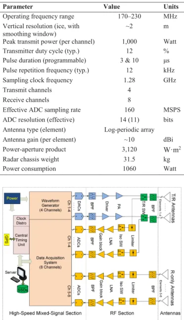
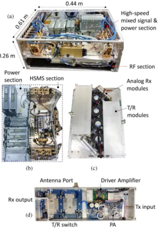
Table I presents a summary of instrument parameters and Fig. 1 presents a simplified block diagram of the system, which is composed of high-speed mixed signal (HSMS) section, an RF section, and a set of antennas. We housed the radar electronics and the power section (consisting of a set of highly efficient, low-noise switching power supplies) in a compact chassis that weighs less than 32 kg. Fig. 2 shows photographs of the radar chassis and its various parts. We divided the radar’s main en- closure (Fig. 2(a)) into two separate compartments to achieve
4The product of the aperture area and the average transmit power.
TABLE I
SUMMARY OFSYSTEMPARAMETERS
Fig. 1. Simplified system block diagram [20].
high isolation between the RF section and the rest of the system.
The total weight of the radar electronics, including the control server and peripherals, is close to 65 kg, which is significantly lower than the previously developed systems of comparable capabilities. For example, the systems reported in [15]–[18]
weigh 180–300 kg.
A. High-Speed Mixed Signal Section
The system’s HSMS section includes a multichannel wave- form generator and data acquisition system from remote sensing solutions (RSS) [35] and custom clock generation/distribution circuitry. We use a stable 10-MHz source as the base clock signal for the entire system and a phase-locked 1.28-GHz synthesizer as the sampling clock signal source for the RSS modules.
Fig. 2. Photographs of the radar system electronics. (a) Main chassis. (b) Detailed view of the top compartment enclosing the power supplies and HSMS section. (c) Detailed view of the bottom compartment housing the RF section.
(d) Detailed view of one of the improved T/R modules.
The waveform generator is based on digital-to-analog converter chips with 14-b resolution. With these chips, the system is capable of producing RF pulsed signals on four independently programmable channels. In the nominal operation mode, we alternate between pulses of different durations (3 and 10μs) to capture radar returns from shallow and deep internal layers. The nominal operating frequency range is 170–230 MHz, but the system can support other bandwidths and pulse durations.
The data acquisition system features a set of digital receivers to record signals from eight separate antenna elements. This enables array-processing techniques after data collection. The analog-to-digital converters (ADCs) in the data acquisition system are based on a commercial chip with 11-b effective resolution (at 170 MHz) and a full-scale amplitude of 2 Vpp.
We use an internal clock divider to achieve a sampling rate of 640 MSPS and field-programmable array based onboard (×4) decimation with 256 presums to lower the data rate to 13 MB/s (∼46 GB/h) and support long-lasting surveys. We achieve timing and synchronization within this section by using a phase-locked central timing unit. We use an external global positioning system receiver to geo-locate the data in postprocess- ing. Lastly, we employ a high-performance computing server for instrument control, data storage, real-time A-scope (amplitude versus range) display for data quality checks, and off-line data backups and processing. The different blocks within this section
exchange data using the user datagram protocol via Ethernet network interfaces [20].
B. RF Section
The radar’s RF section includes four transmit/receive (T/R) channels and four, dual channel analog receiver modules. An important component of the radar system is a bank of fast- switching, low-loss T/R switches with high peak power ca- pabilities and high isolation. We use them as duplexers for the antennas, thereby sharing them for alternating transmit and receive events. The switch design is an enhanced version of the implementation presented in [37], with higher transmit power and faster switching time in a lighter weight module. It is based on P-type, intrinsic, N-type diodes in a balanced configuration.
The transmitter circuitry provides frequency selectivity and am- plifies the signals from the waveform generator before feeding the antennas via low-loss coaxial cables.
Each transmit channel has a total power gain of approximately 60 dB and a peak output power of 1000 W (60 dBm), which results in a combined peak transmit power of 4000 W (66 dBm).
Each transmit channel includes a two-stage 50-W pulsed driver stage and a power amplifier pallet from a commercial vendor, which we operated in class B mode with 25 mA of quiescent currentIDQ. Such low value ofIDQhelps reduce the amplifier’s dc-power consumption while achieving acceptable linearity lev- els and preventing amplified thermal noise from being injected into the receiver outside the transmit event. The active devices in the transmitter are based on laterally diffused metal-oxide semiconductor transistors. We typically drive them at 12% duty cycle (120 W average per channel).
The analog receiver modules condition the signals collected by the antennas before the data acquisition system records them. They include power limiters and blanking switches to protect them from damage during high-power transmissions and saturation within the first few microseconds that follow the transmit event. The receiver modules have a nominal noise figure of 2.5 dB and a gain of 48 dB, which is set to bring their output noise level of 6–10 dB above the quantization noise of the ADCs, thereby maximizing the system’s dynamic range.
With full gain, the receivers can capture signals as low as the MDS (∼−170 dBm assuming 51 200 integrations) and as high as−38 dBm before the ADCs reach their full scale.
C. Antennas and Survey Platform
To achieve a large effective aperture size, we employ a set of eight downward-looking antennas with high gain. We use two subarrays, each consisting of four (18-element) log-periodic structures. One of the subarrays is used for duplexed transmit and receive operations, while the second subarray is used for reception only. The antennas have an individual gain of 10.1 dBi andE- andH-plane beamwidths of 53 ° and 67 °, respectively.
The gain for the four-element transmit array is 15.6 dBi, which corresponds to an effective aperture area of 6.5 m2. With 4 kW of peak transmit power at a duty cycle of 12%, the total average power is 480 W. The power-aperture product for the system is thus 3120 W·m2.
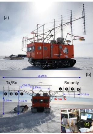
Fig. 3. (a) Photograph of the Ohara SM100 vehicle equipped with high-gain log-periodic antennas during field operations in Antarctica. (b) Details of the antenna array geometry. The labels UA Tx/Rx correspond to the transmit and receive antennas of a microwave radar system for near-surface layer mapping [36], which was operated in conjunction with the radar depth sounder. (c) Photograph of the radar system installed inside the vehicle’s cabin. We used cushion foam sheets combined and shock-absorbing mounts to minimize the effect of vehicle vibrations in the radar electronics.
We attached the antenna elements to a custom-made mounting structure, placing one subarray at either sides of the diesel- engine heavy snow tracked vehicle (Ohara SM100 S-type) pro- vided by the JARE team. Fig. 3 shows the antenna configuration and setup. The spacing between antennas within a subarray is
∼1 m. The antennas are linearly polarized with the polarization plane parallel to the tracked vehicle.
IV. LABORATORYTESTS ANDPERFORMANCE
A. Laboratory Tests
We conducted a series of tests in a laboratory environment to validate the capabilities of the radar system prior to deployment.
First, we evaluated the transmit waveform qualities by setting the AWG to produce a 170–230 MHz linear frequency-modulated up-chirp with a 0.1 Tukey envelope and captured the transmitter output waveform using a fast-digitizing oscilloscope. We used a high-power attenuator (50 dB) to bring the signal down to a safe input range for the oscilloscope. Fig. 4(a) shows the captured waveform for a single transmitter, which has a max- imum amplitude of 2 Vpp and corresponds to 1000-W peak after correcting for the losses in the test setup. The rolloff in the signal envelope is due to the frequency-dependent gain of
Fig. 4. Transmitter output waveform (a) without and (b) with digital pre- emphasis. We captured these signals after a 50-dB high-power attenuator.
(c) Oscilloscope screen capture showing the transition time through the receive–
transmit–receive states in the T/R switch.
the transmitter chain. The four transmitter channels exhibited similar behavior. The AWG supports digital pre-emphasis to compensate for the amplitude rolloff on a per-channel basis.
Fig. 4(b) shows the transmitter output waveform after using digital pre-emphasis, which results in a flat peak power profile of 1000 W across the pulse duration.
We also verified the transition time going from transmit and receive states in the T/R switch. Fast switching is important to minimize the system’s “blind” range. To this end, we injected a continuous-wave signal into the antenna port of the switch and monitored its receive port’s output signal as the switch control signal was toggled between states. Fig. 4(c) shows the waveform obtained in the oscilloscope, indicating a switch time of 440 ns.
The final specifications of the T/R switches employed in this system exceed those of similar circuits reported in the literature [16], [38]–[40], with the added advantage of not requiring large negative biasing voltages.
Next, we measured the receiver noise figure using the Y-factor technique. We did this to verify the lower end of the receiver’s dynamic range. We employed a calibrated noise source with ex- cess noise ratio of 15.2 dB at 200 MHz. We measured a Y-factor of 13.1 dB, which corresponds to a noise figure of 2.31 dB, in agreement with design considerations. We observed comparable behavior among the eight analog receiver modules. Lastly, we evaluated the system’s sensitivity and impulse response by using a synthetic target built upon an electro-optical transceiver and a
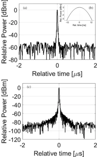
Fig. 5. Measured system response for a receive-only channel (#6) for different test cases: (a) 256 onboard presums and no additional averages with (b) a zoomed-in view of the response’s main lobe. (c) 256 onboard averages with 2000 coherent averages in postprocessing. We obtained the plots after 10× oversampling using Fourier interpolation and Hanning window in the frequency domain.
fiber-optic line with∼25-μs delay. We employed attenuators, a 6-dB directional coupler, and two-way power divider to direct the chirp signal flow and simultaneously exercise individual pairs of T/R channels. All of these measurements were carried out for each of eight channels to ensure the desired performance.
B. System Performance
Fig. 5(a) shows the measured radar response for one of the R-only channels (#6) after pulse compressing a 10-μs-long chirp pulse captured with 256 onboard presums and no off-line averages. The signal is detected with 59.8-dB SNR considering the average of the noise level across 10 001 range bins. With 145 dB of power loss in the setup (excluding cable losses), the LS inferred from these results is 204.8 dB, which is consistent with that obtained for other channels. WithPt=1000 W (with one transmit channel being considered) andNave=256, theory predicts an LS of 205.8 dB, which is within 1 dB from the values inferred from Fig. 5(a). We attribute the difference to the cable losses that we neglected in the estimation of the total loop loss.
Another figure of merit that we assessed from these tests is the range resolution. Fig. 5(b) shows the half-power width of the main lobe to be 23.8 ns, which corresponds to a range resolution of 3.57 m in free space (2.01 m in ice). This figure is in accordance with the theoretical value of 3.60 m (2.03 in ice) given byktc/2B√εr, withktbeing the windowing factor (kt= 1.44),cbeing the velocity of propagation in free space,Bbeing the signal’s bandwidth, andεrbeing the relative permittivity of the media (εr=1 for free space orεr=3.15 for ice).
Next, we quantified the SNR improvement obtained by av- eraging a very large number of records. Fig. 5(c) shows the pulse-compressed signal obtained for the same receive-only channel after averaging 2000 traces in postprocessing. The average noise floor in this plot is−89.5 dB below the signal’s peak, which, for the same 145-dB loss, corresponds to 234.5 dB of LS. The expected LS for these test conditions is 238.8 dB.
After considering the 1-dB losses attributed to interconnects as discussed above, the measured LS is within a few dB of the value predicted by theory (same order of magnitude: 3.55 × 10²³versus 7.53×10²³).
V. FIELD OPERATIONS ANDEXPERIMENTALRESULTS
A. Field Operations
We operated the radar system and collected data over fine- scale grids in three areas near Dome Fuji. The nominal grid spacing varied between 0.5 and 1.0 km, with a total surveyed distance of∼2000 km. We covered∼1400 km during the Dome Fuji survey and 600 km along the traverse. The duration of the deep field operations was∼1 month.
B. Sample Results With Unfocused SAR Processing
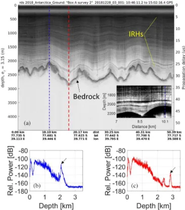
While in the field, we completed first-order processing for on-site assessment of data quality. Fig. 6(a) shows an example of a field-processed radar image from this data set, covering 50.4 km. The inset shows a zoomed view of the basal structure between kilometer markers 7 and 10.5 along the survey line. We employed an unfocused SAR processing algorithm implemented in the CReSIS toolbox [41], in which we only perform stacking.
We combined the 3- and 10-μs waveforms and the signals from the eight receiver channels to improve SNR but did not yet apply corrections for interchannel phase and amplitude mismatches.
We used 20 coherent averages and decimation by 20, along with 10 incoherent averages and decimation by a factor of 10. With these preliminary processing settings, the radar instrument was able to map the ice–bed interface at depths ranging from 2 to
∼3 km, while providing internal layer information from a depth of 300 m down to withinca.100 m from the bed. The obscured region in the first 300 m is expected and due to the toggling of the T/R and blanking switches mentioned in Section IV-A.
We picked two different locations in this frame to illustrate the detection capabilities of the system. The first one corresponds to a location approximately 10 km from the start of the line (marked by the blue vertical line), where the ice thickness is∼2 km. The second range line is marked in red, in which the bed is∼2.8 km
Fig. 6. (a) Field-processed echogram from UWB radar data collected on December 28, 2018 over a 50-km stretch. The inset shows a zoomed-in view of the ice structure near the bed for a subsection of the survey line. (b) A-scope for a range line∼10 km from the start of the line (marked in blue). (c) A-scope for the area with the thickest ice within the frame (marked in red). The radar returns from the bed are marked with black arrows.
below the surface. Fig. 6(b) and (c) presents the relative received power in dB (A-scopes) for the two abovementioned lines (blue and red, respectively). The SNRs for these two bed echoes are 58 and 35 dB, respectively.
C. Comparison With Other Surface-Based Measurements Alongside the newly developed radar depth sounder, a sepa- rate subteam deployed a pulse-modulated VHF radar onboard a different tracked vehicle to maximize the survey coverage. The second radar was provided by the Japanese National Institute of Polar Research (NIPR).
The NIPR radar is also equipped with high-gain antennas5 and is capable of transmitting different pulse widths6 to diagnose internal layer conditions with either higher SNR or finer resolu- tion. It operates at a center frequency of 179 MHz with a peak transmit power of 1000 W and a pulse repetition frequency of 1 kHz. It has an MDS of−110 dBm, which translates into an LS of 170 dB with 60 dBm of transmit power. The NIPR radar has been used extensively in previous studies [10], [26]–[29], [32].
Although there was not a complete coverage overlap between
5This system was equipped with two 16-element Yagi antennas with 17-dBi gain dedicated for transmission and the same number of elements for reception.
6The selectable pulse durations are 250 and 60 ns, resulting in a vertical resolution of 21 and 5 m, respectively.
the two systems, having a second radio-echo sounder operating in the same area provides a completely independent data set and a valuable verification tool at the crossover points.
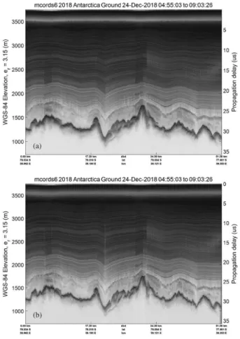
Fig. 7(a) shows a small subset of the survey grid, which includes four neighboring paths mapped with three different systems. The trajectory marked in black was mapped using the CReSIS UWB radar. The blue/gray lines were surveyed with the NIPR system. These lines are parallel to each other with a separation of 0.5–1.2 km. The green line represents part of an airborne survey conducted with the AWI’s legacy RES system [14], [30]. We will discuss the data from this line in Section V-D.
Fig. 7(b) shows a radar image from data collected with the UWB system (frame 20181224-03-01) while Fig. 7(c) and (d) shows two radar images from data collected with the NIPR sys- tem (frames 20181221-1222 and 20181225, respectively). The minimum ice thickness values obtained in this area are slightly less than 1.97 km, while the maximum measured ice depth is 2.63 km. The thickness differences over 13 crossover points ranged from 4.4 to 28.2 m, with the average difference being
∼16 m (less than 1%). These are representative results to show that both systems produce comparable thickness ranges, thereby verifying the satisfactory performance of the new system. We are in the process of performing a more detailed comparison between the two data sets over a larger area and constructing an enhanced basal topographic map [42].
D. Comparison With Airborne Data
We performed two types of comparisons with airborne mea- surements. First, we assessed the ice thickness values obtained from the UWB and NIPR systems in relation to the AWI airborne measurements [30]. We relied on two previous inde- pendent analyses comparing the raw data sets from the AWI 2016/2017 and the JARE 2017/2018 campaigns, which revealed average differences in ice thickness in the 11–16 m range over many crossing points. These differences are consistent with the results from our preliminary crossover analysis, discussed in Section V-C.
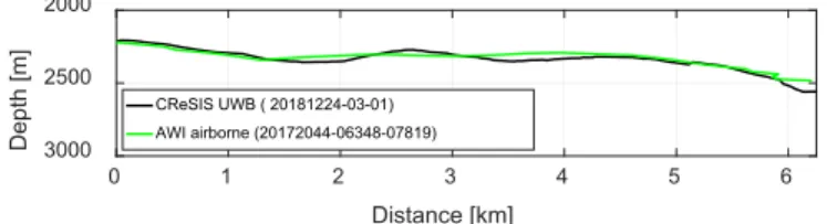
Second, we assessed differences in ice thickness and mapping of IRHs at a finer scale by comparing data from the UWB (frame 20181224-03-01) versus data collected during the 2016/2017 AWI aerial survey (frame 20172044-06348-07819). Fig. 7(e) shows the echogram from the airborne data acquisition along the (∼50-km long) green line of Fig. 7(a), using the system’s coarse 600-ns pulse. At∼22 km from the start of the surveys, the airborne and UWB terrestrial radar acquisitions practically overlap over a 6–7 km long segment (∼0.1 km offset). Fig. 8 shows the comparison of the two ice thickness profiles across the middle section of the overlap area. The ice thickness in this region ranges between 2.2 and 2.5 km. Both systems produced comparable ice depth profiles (correlation coefficient>0.91), with an average thickness difference of less than 1%.
E. Focused SAR Results
Fig. 9 shows a comparison between an unfocused SAR image (Fig. 9(a)) and a fully SAR processed image after systematic
Fig. 7. (a) Semicoincident survey trajectories used for data comparisons between three different radar systems. (b) Quick-look processed echogram from data collected with the CReSIS’ UWB radar over the black line (frame 20181224-03-001). (c) Echogram from data collected with the NIPR radar over the blue line (frame 20181221-1222). (d) Echogram from data collected with the NIPR radar over the grey line (frame 20181225). (e) Echogram collected over the green line with the AWI’s airborne RES system configured with a coarse 600-ns burst (frame 20172044-06348-07819).
Fig. 8. Comparison of the ice thickness inferred from the CReSIS UWB data (frame 20181224-03-01) and AWI’s airborne data (frame 20172044-06348- 07819).
corrections (Fig. 9(b)). The processing employed to obtain Fig. 9(b) follows steps similar to those described in [41] for the standard SAR focused data product. The data from each channel are pulse compressed using an ideal matched filter with a Hanning smoothing window in the frequency domain. The phase and amplitude of each channel are then adjusted based on calibration measurements that remove phase and amplitude dif- ferences between the channels caused by cable and component mismatches. Each channel is then SAR processed using thef–k migration algorithm described in [43], in which we assume a dielectric half-space of air and ice and do not account for the snow–firn transition.
The first step includes array processing using delay and sum for a nadir squint angle. Since all antennas are (nominally) at
the same horizontal level, there is no need to delay the channels to align them and only summing is necessary. Because of the large offset between the two arrays of antennas, we incoherently combine the SAR processed data from the two arrays. Data from the left four antennas and right four antennas are array processed separately (coherently summed). The multilooking process power detects each of these coherently summed data and then sums them together in addition to doing a neighborhood multilooking with 11 along-track pixels (five range lines ahead and five range lines behind). No multilooking is done in the fast-time (range) dimension to ensure that layer resolution is not compromised. The final step is to merge the SAR processed data into a single image. We combine the 3-μs multilooked data with the 10-μs data at 10-μs two-way travel time so that the image shown in Fig. 9(b) uses the 3-μs data for the top or near-surface part of the echogram and the 10-μs data for the bottom or deeper part of the image.
The echogram is distorted for fast-time range bins of less than 3 μs because the receivers are blanked, as in the unfo- cused images presented in Figs. 6(a), 7(b), and 9(a). Another characteristic of the unfocused images is the presence of range hyperbolas in the ice–bed interface and broadening of the bed returns, resulting in potential biases in ice thickness information.
After SAR processing, Fig. 9(b) provides a refined data product that we can use for a more accurate determination of basal conditions and internal layer tracking.
Fig. 9. Comparison between the (a) unfocused SAR image for frame 20181224-03-001 and the (b) fully processed SAR image for the same frame.
VI. CONCLUSION
We developed a portable, UWB ice imaging radar system with sensitivity exceeding 230 dB and vertical resolution of∼2 m in ice. Our laboratory tests revealed that its detection performance is only slightly lower than our theoretical expectations. We used the system onboard a large tracked vehicle equipped with high-gain antennas to obtain a power-aperture product greater than 3000 W·m2, thereby achieving the performance required to map the ice–bed interface and IRHs in the Dome Fuji area in East Antarctica. We acquired a detailed ice thickness data set with values that qualitatively match those obtained by a pulse- modulated VHF radar system deployed in tandem as well as earlier airborne measurements. We presented a fully processed radar image as an example of the final data product that will be available to the science community. The compact UWB radar system described in this article offers fine vertical resolution data all the way to the basal section of the ice column, whereOldest Icecan possibly be present. We will further evaluate these radar results alone and with ice-flow models in order to narrow the location of candidate sites forOldest Icedrilling.
ACKNOWLEDGMENT
The authors would like to thank the entire USA–Japan–
Norway collaborative team. The authors would like to gratefully acknowledge A. Paden, K. T. Karidi, B. Shang, P. Place, H.
Ailon, and S. Alvarez, and others at the University of Kansas for their work assembling and testing the radar system. The authors would like to thank T. Akins and J. Carswell at Remote Sensing Solutions for their work on the radar’s waveform generator and data acquisition systems and R. Taylor at the University of Alabama for project coordination and support. A. R. Harish and G. Gupta at the Indian Institute of Technology, Kanpur are recognized for valuable input to the antenna array design. The authors would like to recognize C. O’Neill at the University of Alabama for identifying the foam used for vibration dampening.
The authors also acknowledge support from the various entities that financed the instrument development and field operations. In particular, this work would not have been possible without sup- port for the Center for Remote Sensing of Ice Sheets (CReSIS) Science and Technology Center by the U.S. National Science Foundation between 2005 and 2017. Japanese activities were supported by the National Institute of Polar Research under MEXT. Ground traverse team from Japanese Syowa Station to Dome Fuji was organized and managed by the wintering team of the 59th Japanese Antarctic Research Expedition led by N.
Kizu and by the 60th Japanese Antarctic Expedition led by M.
Tsutsumi. The authors acknowledge logistics members in the inland traverse, T. Ito, H. Kaneko, S. Sakurai, S. Takamura, and Y. Okada for their generous support during the traverse, to make both the long traverse and the radar observations real. The authors also acknowledge T. Tsubaki and T. Takase at Ohara Corporation for providing the generator mounting system on tracked vehicles for the radars. Air operations were carried out by the British Antarctic Survey with field support by the Interna- tional Polar Foundation (IPF) at the Belgian Princess Elisabeth Station (PEA), and the Norwegian Troll Station, in the frame of Beyond EPICA-Oldest Ice (BE-OI). F. Pattyn generated extra funding from the Belgian Federal Science Policy Office for field support at PEA. BE-OI has received funding from the European Union’s Horizon 2020 research and innovation program under Grant 730258 (BE-OI CSA). This work was also supported by KAKENHI from the Japan Society for the Promotion of Science and MEXT under Grant 17H06320, Grant 17H06104, and Grant 18H05294. The authors would like to gratefully acknowledge the support received from the Norwegian Polar Institute. Lastly, the authors would like to thank the two anonymous reviewers whose input helped us improve this article.
REFERENCES
[1] L. Augustinet al., “Eight glacial cycles from an Antarctic ice core,”
Nature, vol. 429, 2004, pp. 623–628. Available: https://doi.org/10.1038/
nature02599
[2] K. Kawamuraet al., “State dependence of climatic instability over the past 720,000 years from Antarctic ice cores and climate modeling,”Sci. Adv., vol. 3, no. 2, Feb. 2017, Art. no. e1600446.
[3] P. Clarket al., “The middle Pleistocene transition: Characteristics, mech- anisms, and implications for long-term changes in atmospheric pCO2,”
Quat. Sci. Rev., vol. 25, no. 23-24, pp. 3150–3184, 2006.
[4] B. Van Liefferinge and F. Pattyn, “Using ice-flow models to evaluate potential sites of million year-old ice in Antarctica,”Clim. Past, vol. 9, pp. 2335–2345, 2013.
[5] B. Van Liefferingeet al., “Promising oldest ice sites in East Antarc- tica based on thermodynamical modeling,” Cryosphere, vol. 12, pp. 2773–2787, 2018.
[6] H. Fischeret al., “Where to find 1.5 million yr old ice for the IPICS
“Oldest-Ice” ice core,”Clim. Past, vol. 9, pp. 2489–2505, 2013. Available:
https://doi.org/10.5194/cp-9-2489-2013
[7] S. Fujita and S. Mae, “Causes and nature of ice-sheet radio-echo internal reflections estimated from the dielectric properties of ice,”Ann. Glaciol., vol. 20, pp. 80–86, 1994.
[8] O. Eisen, F. Wilhelms, D. Steinhage, and J. Schwander, “Improved method to determine radio-echo sounding reflector depths from ice-core profiles of permittivity and conductivity,”J. Glaciol., vol. 52, no. 177, pp. 299–310, 2006.
[9] O. Eisen, I. Hamann, S. Kipfstuhl, D. Steinhage, and F. Wilhelms, “Di- rect evidence for continuous radar reflector originating from changes in crystal-orientation fabric,”Cryosphere, vol. 1, pp. 1–10, 2007. Available:
https://doi.org/10.5194/tc-1-1-2007
[10] S. Fujita, “Development and use of ice sounding radars in the Japanese Antarctic research expedition,” Antarctic Rec., vol. 52 (special issue), pp. 238–250, May 2008.
[11] C. Allen, “A brief history of radio-echo sounding of ice,” Earthzine.
Available: https://earthzine.org/a-brief-history-of-radio-echo-sounding- of-ice-2/
[12] S. Popov, “Fifty-five years of Russian radio-echo sounding inves- tigations in Antarctica,” Ann. Glaciol., pp. 1–11, Feb. 2020, doi:
10.1017/aog.2020.4.
[13] S. Hodge, D. Wright, J. Bradley, and R. Jacobel, “Determination of the surface and bed topography in central Greenland,”J. Glaciol., vol. 36, no. 122, pp. 17–30, 1990.
[14] U. Nixdorfet al., “The newly developed airborne radio-echo sounding sys- tem of the AWI as a glaciological tool,”Ann. Glaciol., vol. 29, pp. 231–238, 1999.
[15] C. Allen, J. Paden, D. Dunson, and P. Gogineni, “Ground-based multi- channel synthetic-aperture radar for mapping the ice-bed interface,” in Proc. IEEE Radar Conf., Rome, Italy, May 26–29, 2008, pp. 1428–1433.
[16] F. Rodriguez-Moraleset al.,“ Advanced multi-frequency radar instrumen- tation for polar research,”IEEE Trans. Geosci. Remote Sens., vol. 52, no. 5, pp. 2824–2842, May 2014.
[17] C. Allenet al., “Antarctic ice depthsounding radar instrumentation for the NASA DC-8,”IEEE Aerosp. Elect. Sys. Mag., vol. 27, no. 3, pp. 4–20, Mar. 2012.
[18] Z. Wanget al., “Multichannel wideband synthetic aperture radar for ice remote sensing: Development and first deployment in Antarctica,”IEEE J. Sel. Top. App. Earth Obs. Remote Sens., vol. 8, no 11, pp. 980–993, Nov. 2015.
[19] F. Sabath, E. Mokole, and S. Samaddar, “Definition and classification of ultrawideband signals and devices,”URSI Radio Sci. Bull., vol. 313, pp. 12–26, Jun. 2005.
[20] F. Rodriguez-Moraleset al., “A compact, multi-channel radar for>1Ma old ice core site identification in East Antarctica, inProc. IEEE Geosci.
Remote Sens. Int. Symp., Yokohama, Japan, 2019, pp. 4161–4164.
[21] K. Shiraishi, “Dome Fuji station in East Antarctica and the Japanese Antarctic research expedition,”Proc. Int. Astron. Union, vol. 8, no. S288, pp. 161–168, 2012.
[22] T. Kameda, N. Azuma, T. Furukawa, Y. Ageta, and S. Takahashi, “Surface mass balance, sublimation and snow temperature at Dome Fuji Sta- tion Antarctica,” inProc. NIPR Symp. Polar Meteorol. Glaciol., 1997, pp. 24–34.
[23] O. Watanabe, J. Jouzel, S. Johnsen, F. Parrenin, H. Shoji, and N. Yoshida,
“Homogeneous climate variability across East Antarctica over the past three glacial cycles,”Nature, vol. 422, pp. 509–512, 2003.
[24] T. Kamedaet al., “Temporal and spatial variability of surface mass balance at Dome Fuji, East Antarctica, by the stake method from 1995 to 2006,”
J. Glaciol., vol. 54, no. 184, pp. 107–116, 2008.
[25] A. Svenssonet al., “On the occurrence of annual layers in Dome Fuji ice core early Holocene ice,”Clim. Past., vol. 11, pp. 1127–1137, 2015.
[26] S. Fujitaet al., “Radar diagnosis of the subglacial conditions in Dronning Maud Land, East Antarctica,” Cryosphere, vol. 6, no. 5, 1203–1219, 2012.
[27] S. Fujitaet al., “Nature of radio-echo layering in the Antarctic Ice Sheet detected by a two-frequency experiment,” J. Geophys. Res., vol. 104, no. B6, pp. 13013–13024, 1999.
[28] K. Matsuokaet al., “Crystal orientation fabrics within the Antarctic Ice Sheet revealed by a multipolarization plane and dual-frequency radar survey,”J. Geophys. Res., vol. 108, no. B10, 2003, Art. no. 2499.
[29] S. Fujitaet al., “Spatial and temporal variability of snow accumulation rate on the East Antarctic ice divide between Dome Fuji and EPICA DML,”
Cryosphere, vol. 5, pp. 1057–1081, 2011.
[30] N. Karlssonet al., “Glaciological characteristics in the Dome Fuji region and new assessment for “Oldest Ice”,”Cryosphere, vol. 12, pp. 2413–2424, 2018. Available: https://doi.org/10.5194/tc-12-2413-2018
[31] N. Karlssonet al.,Ice Thickness from the Dome Fuji Region, East Antarc- tica from Ice-Penetrating Radar. Bremerhaven, Germany: Alfred Wegener Institute, Helmholtz Centre for Polar and Marine Research, PANGAEA.
Available: https://doi.org/10.1594/PANGAEA.891323
[32] K. Matsuoka, H. Maeno, S. Uratsuka, S. Fujita, T. Furukawa, and O. Watanabe, “A ground-based, multi-frequency ice-penetrating radar system,”Ann. Glaciol., vol. 34, pp. 171–176, 2002.
[33] P. Gogineni and J.-B. Yan, “Remote sensing of ice thickness and surface velocity,” inRemote Sensing of the Cryosphere. Hoboken, NJ, USA: John Wiley and Sons, Nov. 2014, pp. 187–230.
[34] G. de Q. Robin, S. Evans, and T. Bailey, “Interpretation of radio echo sounding in polar ice sheets,”Philos. Trails. R. Soc. London Ser., A, vol. 265, no. 1166, pp. 437–505, 1969.
[35] Remote Sensing Solutions. Accessed: Mar. 26, 2020. [Online]. Available:
https://remotesensingsolutions.com/
[36] R. Tayloret al., “A prototype ultra-wideband FMCW radar for snow and soil-moisture measurements,” inProc. IEEE Geosci. Remote Sens. Int.
Symp., Yokohama, Japan, 2019, pp. 3974–3977.
[37] F. Rodriguez-Moraleset al., “Wideband transmit/receive switches and modules for ice sounding/imaging radar,”Microw. J., vol. 59, no. 5, pp. S6–S18, May 2016.
[38] E. L. Christensen, N. Reeh, R. Forsberg, J. H. Jørgensen, N. Skou, and K. A. Woelders, “A low-cost glacier-mapping system,”J. Glaciol., vol. 46, no. 154, pp. 531–537, Aug. 2000.
[39] M. E. Peters, D. D. Blankenship, and D. L. Morse, “Analysis techniques for coherent airborne radar sounding: Application to West Antarctic ice streams,”J. Geophys. Res. Atmos., vol. 110, no. 6, pp. 1–17, Jun. 2005.
[40] C. C. Hernandez, V. Krozer, J. Vidkjaer, and J. Dall, “Design and per- formance of an airborne ice sounding radar front-end,” inProc. Microw.
Radar Rem. Sens. Symp., Sep. 2008, pp. 284–288.
[41] CReSIS. 2018. CReSIS Toolbox. [Computer Software]. Lawrence, Kansas, USA. Available: https://git.cresis.ku.edu/ct/
[42] S. Tsutaki et al., “A basal topographic map in the Dome Fuji area, East Antarctica, constructed from a ground-based radar survey,” inProc.
Jpn. Geosci. Union Amer. Geophys. Union Joint Meeting, Chiba, Japan, May 2020.
[43] C. Leuschen, S. Gogineni, and D. Tammana, “SAR processing of radar echo sounder data,” inProc. IEEE Geosci. Remote Sens. Int. Symp., vol. 6, 2000, pp. 2570–2572.
Fernando Rodriguez-Morales (Senior Member, IEEE) received the B.S. degree in electronics engi- neering from the Universidad Autónoma Metropoli- tana, Mexico City, Mexico, in 1999, and the M.S. and Ph.D. degrees in electrical and computer engineering from the University of Massachusetts, Amherst, MA, USA, in 2003 and 2007, respectively.
Since 2007, he has been with the Center for Remote Sensing of Ice Sheets (CReSIS), University of Kansas (KU), Lawrence, KS, USA, where he is currently a Research Faculty Member and holds a courtesy ap- pointment with the Department of Electrical Engineering and Computer Science.
He has conducted extensive fieldwork in Antarctica, Greenland, Iceland, Alaska, and Patagonia. His current technical interests include extending the capabilities of UWB radar instruments, as well as packaging, miniaturization, and hardening of advanced high-frequency systems.
Dr. Rodriguez-Morales was a recipient of graduate fellowships from Mexico’s National Institute for Astrophysics, Optics and Electronics (INAOE) and the National Council for Science and Technology (CONACyT), the U.S. Antarctic Service Medal, and three NASA agency honor awards.
David Braaten(Member, IEEE) received the B.S. de- gree in meteorology from the State University of New York, Oswego, NY, USA, in 1977, the M.S. degree in meteorology from San Jose State University, San Jose, CA, USA, in 1981, and the Ph.D. in atmospheric science from the University of California, Davis, CA, USA, in 1988.
He is currently a Professor with the Department of Geography and Atmospheric Science, University of Kansas (KU), Lawrence, KS, USA, where he has been teaching atmospheric science since 1989. He is associated with the Center for Remote Sensing of Ice Sheets, KU, with an interest in snow accumulation processes and ice sheet mass balance.
Hoang Trong Maireceived the B.S. degree in electri- cal engineering from the University of Kansas (KU), Lawrence, KS, USA, in 2020. He is currently working toward the M.S. degree in electrical engineering at KU, specializing in radar systems.
Since 2019, he has been a Graduate Research Assistant with the Center for Remote Sensing of Ice Sheets (CReSIS), KU, where his current work focuses on the development of high-frequency com- ponents and power circuitry for radar remote sensing instruments.
John Paden(Senior Member, IEEE) received the M.Sc. and Ph.D. degrees in electrical engineering from the University of Kansas (KU), Lawrence, KS, USA, in 2003 and 2006, respectively, studying radar signal and data processing for remote sensing of the cryosphere.
After graduating, he joined Vexcel Corporation, Boulder, CO, USA, a remote sensing company, where he worked as a Systems Engineer and an SAR Engi- neer for three and a half years before rejoining the Center for Remote Sensing of Ice Sheets (CReSIS), KU, in early 2010 to lead the radar signal and data processing efforts.
Dr. Paden was the recipient of the American Geophysical Union Cryosphere Early Career Award, in 2016. He was also the recipient of three NASA group achievement awards for radio glaciology work. He is currently a research faculty member at CReSIS.
Prasad Gogineni(Fellow, IEEE) received the Ph.D.
degree in electrical engineering from the University of Kansas (KU), Lawrence, KS, USA, in 1984.
He is currently the Cudworth Professor with the Department of Electrical and Computer Engineering and the Department of Aerospace Engineering and Mechanics, and the founding Director of the Remote Sensing Center, University of Alabama, Tuscaloosa, AL, USA. He was formerly a Deane E. Ackers dis- tinguished Professor with KU, where he was also the Founding Director of the National Science Foun- dation Science and Technology Center for Remote Sensing of Ice Sheets.
He developed concepts and early versions of several radar systems that are currently being used at KU for the sounding and imaging of polar ice sheets.
He has also participated in field experiments in the Arctic and Antarctica. He has authored or coauthored more than 130 archival journal publications, 200 technical reports, and conference presentations. His current research interests include the application of radars to the remote sensing of the polar ice sheets, sea ice, ocean, atmosphere, and land.
Dr. Gogineni is a member of URSI, the American Geophysical Union, the In- ternational Glaciological Society, and the Remote Sensing and Photogrammetry Society. He was an Editor for theIEEE Geoscience and Remote Sensing Society Newsletterfrom 1994 to 1997.
Jie-Bang Yan(Member, IEEE) received the B.Eng.
(First Class Hons.) degree in electronic and commu- nications engineering from the University of Hong Kong, Hong Kong, in 2006, the M.Phil. degree in electronic and computer engineering from the Hong Kong University of Science and Technology, Hong Kong, in 2008, and the Ph.D. degree in electrical and computer engineering from the University of Illinois at Urbana–Champaign, Champaign, IL, USA, in 2011.
From 2009 to 2011, he was a Croucher Scholar with the University of Illinois at Urbana–Champaign, where he was involved in MIMO and reconfigurable antennas. In 2011, he joined the Center for Remote Sensing of Ice Sheets, University of Kansas, Lawrence, KS, USA, as an Assistant Research Professor. He is currently an Assistant Professor of Electrical and Computer Engineering and the founding Deputy Director of the Remote Sensing Center, University of Alabama, Tuscaloosa, AL, USA. He holds two U.S.
patents and two U.S. patent applications related to novel antenna technologies.
His current research interests include the design and analysis of antennas and phased arrays, ultra-wideband radar systems, radar signal processing, and remote sensing. He also has extensive airborne and ground-based radar deployment experience in both domestic and international regions.
Dr. Yan was the recipient of multiple research awards, including the Best Paper Award, in the 2007 IEEE (HK) AP/MTT Postgraduate Conference, the UIUC Raj Mittra Outstanding Research Award, in 2011, the NASA Group Achievement Award, in 2013, the UA CoE Research and Innovation Award, in 2019, and others. He also serves as a Technical Reviewer for several journals and conferences on antennas and remote sensing.
Ayako Abe-Ouchireceived the B.Sc. and M.Sc. de- grees in geophysics from The University of Tokyo, Tokyo, Japan, in 1987 and 1989. She studied global climate and ice sheet dynamics and received the Ph.D.
degree from the Swiss Federal Institute of Technology (ETH), Zurich, Switzerland, in 1993.
She is a Professor with Atmosphere and Ocean Re- search Institute, The University of Tokyo and special- izes in climate dynamics for the past and future. She is interested in how the climate–ice sheet system re- sponds to external forcing, such as greenhouse gases and the Earth’s orbit (Milankovitch forcing). In order to solve the mechanism of the ice-age cycle, which shifted from a 40–100 thousand years’ cycle one million years ago, she is leading an ice sheet climate modeling team and supporting the Japanese research project of ice core drilling at Dome Fuji in Antarctica.
Shuji Fujitareceived the Ph.D. degree in engineering from the Department of Applied Physics, Hokkaido University, Sapporo, Japan, in 1992.
His research interests include glaciology, physics, and chemistry of ice, as well as climate research based on ice cores. His academic career started in 1987.
Since then, he joined the Japanese Antarctic Research Expedition six times. He is currently a Leader in the division of Polar Meteorology and Glaciology at the National Institute of Polar Research, Tokyo, Japan.
Since 2016, he has been acting as a Chair of the Dome Fuji Ice Core Consortium.
Dr. Fujita is a member of the European Geosciences Union, the Japan Geoscience Union, and the International Glaciological Society.
Kenji Kawamurareceived the B.S. degree in science and the M.S. and Ph.D. degrees in geophysics from Tohoku University, Sendai, Japan, in 1994, 1996, and 2001, respectively.
He has worked on ice core paleoclimatology based on gas measurements at the University of Bern (2002–2004), the Scripps Institution of Oceanogra- phy (2004–2006), Tohoku University (2006–2007), and the National Institute of Polar Research, Tokyo (2007–present), where he is currently an Associate Professor. His research interests include reconstruct- ing and understanding past climatic, atmospheric, and glaciological changes over relatively long timescales such as glacial–interglacial cycles and millennial scales.
Dr. Kawamura is a member of the American Geophysical Union and the Japan Geoscience Union.
Shun Tsutakireceived the master’s and Ph.D. degrees in glaciology from Hokkaido University, Sapporo, Japan, in 2006 and 2011, respectively.
From 2011 to 2017, he worked as a Postdoctoral Researcher with Nagoya University, Hokkaido University, and the Japan Aerospace Exploration Agency.
His research focused on interactions between calving glaciers, lakes, and oceans.
He has worked as a Researcher with The University of Tokyo, Tokyo, Japan, and with the National Institute of Polar Research, Tokyo, Japan. He is currently working on the analysis of bedrock topography and surface mass balance in the Dome Fuji region of East Antarctica.
Brice Van Liefferingereceived the M.Sc. degree (Magna cum Laude) in physical geography from the Université Libre de Bruxelles, Brussels, Belgium, in 2011. He received the Ph.D. degree in earth and environmental sciences, specializing in glaciology, in 2018, focusing on the thermal state of the Antarctic Ice Sheet and the search of promising oldest ice sites.
He pursued his interest in glaciology as a Teaching Assistant. In 2018, he joined the Norwegian Polar Institute, Tromsø, Norway, as a Postdoctoral Re- searcher. His current interests include remote sensing, modeling, and thermal state constraint analysis.
Kenichi Matsuoka received the B.E. degree in physics and the M.S. and Ph.D. degrees in earth envi- ronmental sciences from Hokkaido University, Sap- poro, Japan, in 1995, 1997, and 2002, respectively.
He worked with the Department of Earth and Space Sciences, University of Washington, Seattle, WA, USA, from 2002 to 2010, as a Postdoctoral Fellow and then as a Research Assistant Professor. In 2010, he moved to the Norwegian Polar Institute, Tromsø, Norway, where he has been leading Antarctic glaciol- ogy research as a Senior Research Scientist. He has used airborne and ground-based ice-penetrating radar as the primary tool to elucidate processes that control glacial evolution, decipher glacial history, and assess the ongoing and future behavior of polar regions.
Daniel Steinhage received the Diploma in geo- physics from the Westfälische Wilhelms, University Münster, Münster, Germany, in 1994, and the Ph.D.
degree in geophysics from the University of Bremen, Bremen, Germany, in 2000.
He is a Senior Scientist with the Alfred Wegener Institute, Helmholtz Center for Polar and Marine Re- search, Bremerhaven, Germany, participating in and leading several expeditions in polar regions, perform- ing airborne and ground-based radar surveys. Before becoming coordinator of AWI’s research aircraft, his focus was on processing and interpreting airborne radio-echo sounding data.