Arctic nearshore current dynamics and wave climate under declining sea ice conditions
Potential impacts on sediment pathways
A case study from Herschel Island – Qikiqtaruk, Yukon Coast, Canada
Master thesis
to attain the academic degree
Master of Science (M.Sc.) in GeosciencesSubmitted by
Justus Gimsa
Institute of Geosciences University of Potsdam
Potsdam, November 2019
II
Justus Gimsa
Email: gimsa@uni-potsdam.de
Erstgutachter: Prof. Dr. Hugues Lantuit Telegrafenberg A45 14473 Potsdam Email: hugues.lantuit@awi.de
Zweitgutachter: Dr. George Tanski De Boelelaan 1085 1081 HV Amsterdam Niederlande
Email: george.tanski@vu.nl
III
Table of Contents
Table of Contents ... III Index of Figures ... VI List of Abbreviations and Units ... VIII Zusammenfassung ... IX Abstract ... X
1 Introduction ... 1
1.1 Motivation ... 1
1.2 Objectives ... 3
2 Scientific Background ... 4
2.1 Arctic Ocean and Sea Ice ... 4
2.2 Permafrost Coasts ... 6
3 Study Area ... 9
3.1 Herschel Island and Herschel Basin ... 9
3.2 Location A – 2015 – Simpson Point ... 13
3.3 Location B – 2018 – Catton Point ... 15
4 Methods ... 19
4.1 Measurement Methods Study Location A – 2015 ... 19
4.1.1 Wind ... 19
4.1.2 Sea Ice – Directional Fetch ... 20
4.1.3 Modelled Waves ... 22
4.1.4 Stratification ... 23
4.1.5 Currents ... 24
4.2 Measurement Methods Study Location B - 2018 ... 26
4.2.1 Wind ... 26
4.2.2 Sea Ice – Directional Fetch ... 26
4.2.3 Modelled Waves ... 27
IV
4.2.4 In-Situ Waves ... 27
4.2.5 In-Situ Sea Level ... 28
4.2.6 Stratification ... 28
4.2.7 Currents ... 28
5 Results ... 29
5.1 Results for Study Location A – Simpson Point 2015 ... 29
5.1.1 Wind ... 29
5.1.2 Sea Ice – Directional Fetch ... 31
5.1.3 Modelled Waves ... 32
5.1.4 Stratification ... 34
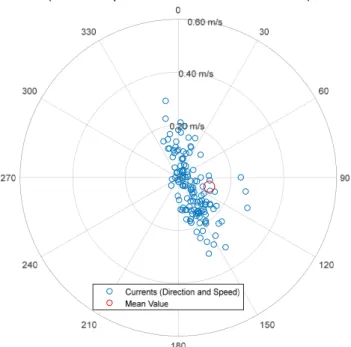
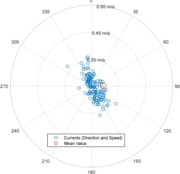
5.1.5 Currents ... 36
5.2 Results for Study Location B – Catton Point 2018 ... 41
5.2.1 Wind ... 41
5.2.2 Sea Ice – Directional Fetch ... 42
5.2.3 Modelled Waves ... 44
5.2.4 Measured Waves ... 46
5.2.5 Measured Sea Level ... 47
5.2.6 Stratification ... 47
5.2.7 Currents ... 48
5.3 Statistical Relationship – Study Location A – 2015 ... 54
5.3.1 Wind Speed and Current Speed ... 55
5.3.2 Modelled Waves and Current Speed ... 62
5.4 Statistical Relationship – Study Location B – 2018 ... 64
5.4.1 Wind Speed and Current Speed ... 65
5.4.2 Modelled Waves and Current Speed ... 71
5.4.3 Measured Waves and Current Speed ... 72
5.4.4 Water Level and Current Speed ... 74
V
6 Discussion ... 77
6.1 Environmental Forcing Conditions ... 77
6.1.1 Wind ... 77
6.1.2 Fetch and Waves ... 77
6.1.3 Stratification ... 78
6.2 Formation of Currents ... 79
6.3 Implications for Sediment Transport ... 83
6.4 Potential Impacts of a Changing Arctic Ocean for the Study Sites ... 84
7 Conclusion ... 85
References ... 86
Appendix ... 98
Acknowledgments ... 99
Selbstständigkeitserklärung ... 100
VI
Index of Figures
1-1 Sketch of processes occurring on eroding permafrost coasts, from Fritz et al. (2017) 1-2 Image of waves approaching to Herschel Island
2-1 Map of circum-Arctic topography and bathymetry, from Jakobsson et al. (2012) 2-2 Map of Arctic currents from Woods Hole Oceanographic Institution (2019)
2-3 Image of an exposed permafrost cliff with marked erosional, from Günther et al. (2013) 3-1 Map of Herschel Island with site location names, from Burn (2012)
3-2 Map of coastal landforms modified from Pelletier & Medioli (2014)
3-3 Map of shoreline change rates along the Yukon Coast, from Irrgang et al. (2018) 3-4 Site photography of Simpson Point, from early August 2018
3-5 Map of Simpson Point shoreline change rates, from Radosavljevic et al. (2016) 3-6 Site picture of Catton Point in 2018
3-7 Map of southern Herschel Island shoreline changes, from Irrgang et al. (2019) 3-8 Bathymetric profiles of the study sites
3-9 Bathymetric model of Herschel Basin, based on bathymetry data from O’Connor (1984) 4-1 Paradigm chart of sea ice product of the Canadian Ice Service (2019)
4-2 Exemplary figure of directional fetch determination
5-1 Time series of wind speed and wind direction at Komakuk Beach in 2015 5-2 Polar scatter plot of the wind distribution at Komakuk Beach in 2015 5-3 Time series of directional fetch and wind direction in 2015
5-4 Polar scatter plots of average directional and maximum potential fetch in 2015 5-5 Time series of modelled wave height and direction in 2015
5-6 Polar scatter plot of the wave distribution in 2015 5-7 CastAway®-CTD measurement profiles in 2015
5-8 Time series of current speed and direction in the upper water column in 2015 5-9 Polar scatter plot of current speed and direction in the upper water column in 2015 5-10 Time series of current speed and direction in the middle water column 2015 5-11 Polar scatter plot of the current distribution in the middle water column in 2015 5-12 Time series of current speed and direction in the lower water column in 2015 5-13 Polar scatter plot of the current distribution in the lower water column in 2015 5-14 Time series of wind speed and wind distribution at Herschel Island in 2018 5-15 Polar scatter plot of wind distribution at Herschel Island in 2018
5-16 Time series of directional fetch and wind direction in 2018
5-17 Polar scatter plots of the average directional and maximum potential fetch in 2018 5-18 Time series of modelled wave height and direction in 2018
5-19 Polar scatter plot of the wave distribution in 2018 5-20 Time series of in-situ wave height measurement in 2018 5-21 Time series of in-situ water depth measurement in 2018 5-22 CastAway®-CTD measurement profiles in 2018
VII
5-23 Time series of current speed and direction in the upper water column in 2018 5-24 Polar scatter plot for the current distribution in the upper water column in 2018 5-25 Time series of current speed and direction in the middle water column in 2018 5-26 Polar scatter plot for the current distribution in the middle water column in 2018 5-27 Time series of current speed and direction in the lower water column in 2018 5-28 Polar scatter plot of the current distribution in the lower water column in 2018 5-29 Multi time series of environmental forcing parameter and current speed 2015 5-30 Scatter plot of wind speed and upper column current speed in 2015
5-31 Scatter plot of wind speed and middle column current speed in 2015 5-32 Scatter plot of wind speed and lower column current speed in 2015
5-33 Scatter plot of wind and upper column current speed in 2015 divided by wind direction 5-34 Scatter plot of wind and middle column current speed in 2015 divided by wind direction 5-35 Scatter plot of wind and lower column current speed in 2015 divided by wind direction 5-36 Scatter plot of wind speed and upper current speed in 2015 divided by fetch length 5-37 Scatter plot of wind speed and middle current speed in 2015 divided by fetch length 5-38 Scatter plot of wind speed and lower current speed in 2015 divided by fetch length 5-39 Scatter plot of wave height and upper column current speed in 2015
5-40 Scatter plot of wave height and middle column current speed in 2015 5-41 Scatter plot of wave height and lower column current speed in 2015
5-42 Multi time series of environmental forcing parameter and current speed 2018 5-43 Scatter plot of wind speed and upper column current speed in 2018
5-44 Scatter plot of wind speed and middle column current speed in 2018 5-45 Scatter plot of wind speed and lower column current speed in 2018
5-46 Scatter plot of wind speed and upper current speed in 2018 divided by wind direction 5-47 Scatter plot of wind speed and middle current speed in 2018 divided by wind direction 5-48 Scatter plot of wind speed and lower current speed in 2018 divided by wind direction 5-49 Scatter plot of wind speed and upper column current speed in 2018
5-50 Scatter plot of wind speed and upper column current speed in 2018 5-51 Scatter plot of wind speed and lower column current speed in 2018
5-52 Scatter plot of modelled wave height and upper column current speed in 2018 5-53 Scatter plot of modelled wave height and middle column current speed in 2018 5-54 Scatter plot of modelled wave height and lower column current speed in 2018 5-55 Scatter plot of wave height measurements and upper column current speed in 2018 5-56 Scatter plot of wave height measurements and middle column current speed in 2018 5-57 Scatter plot of wave height measurements and lower column current speed in 2018 5-58 Scatter plot of water level and upper column current speed in 2018
5-59 Scatter plot of water level and middle column current speed in 2018 6-1 Cumulative vector plot of currents in 2015
6-2 Cumulative vector plot of currents in 2018
VIII
List of Abbreviations and Units
°C Degree Celsius
ADCP Acoustic Doppler Current Profiler
CTD Conductivity Temperature Depth Sonde
E East
h Hour
Hz (1/Second)
kHz Kilohertz
km Kilometer
m Meter
m/a Meter per Year m/s Meter per Second
N North
NOAA National Oceanic and Atmospheric Administration ppt Parts per Thousands
R² Coefficient of Determination
S South
W West
IX
Zusammenfassung
Der durch den Menschen verursachte globale Klimawandel trifft die Arktis in besonderem Maße. Aufgrund der Erwärmungen großer Teile der Erde, verändern sich Atmosphäre, Kryosphäre und Hydrosphäre. Durch diese Veränderungen sind das arktische Ökosystem, Küstensysteme als auch kulturelle Stätten gefährdet.
Die Erwärmung des Klimas in der Arktis führt zur Beschleunigung der Abtragung eisreicher gefrorener arktischer Küstenlinien. Durch den daraus entstehenden Eintrag von Sediment, Nährstoffen, Schadstoffen und organischem Kohlenstoff, verändert sich das gesamte Ökosystem der arktischen Nahküstensysteme und durch die Umsetzung des Kohlenstoffs zu Treibhausgasen auch die Zusammensetzung der globalen Atmosphäre.
In dieser Arbeit wurde mit Hilfe von direkten Messungen der Strömungen im Nahküstengebiet, sowie der Verbindung zu anderen Messungen und Modellierung der Umweltparameter ein allgemeines Lagebild der Strömungen und deren Ursprung erstellt.
Die Strömungen wurden mit Hilfe eines akustischen profilierenden Strömungsmessers (ADCP) für einen kurzen Zeitraum von jeweils zwei Wochen in der westlichen kanadischen Beaufortsee, nahe der Herschel Insel ermittelt und mit Windmessungen, Ergebnissen aus Wellenberechnungen und Wassersäulenschichtungsmessungen verbunden, um deren Einfluss auf die Strömungen festzustellen.
Die Ergebnisse zeigen einen deutlichen Einfluss des Windes auf die Strömung. Dieser Einfluss fällt jedoch je nach Tiefe und Windrichtung unterschiedlich aus und unterliegt somit eines komplexen Gefüges. Darüber hinaus zeigen die Ergebnisse der direkten Wellenmessungen in der zweiten Messung einen deutlichen Einfluss des Meereises auf die Wellenaktivität, sowie eine Reduktion der Strömung, während der Präsenz von Meereis im Studiengebiet, sowie eine Verstärkung der meeresbodennahen Strömung.
Dies kann besonders wichtig für die Verteilung von eingetragener Schwebfracht des nahen Mackenzie Rivers während der Abflussspitze im Frühjahr sein.
Besonders wichtig für die weitere Entwicklung der erodierenden Küsten sind die Richtung und die Geschwindigkeit des abgetragenen Sediments im Nahküstenbereich. Diese Parameter hängen entscheidend von den vorherrschenden Strömungsbedingung in dem Bereich ab. Dadurch können die hier erhobenen und ausgewerteten Daten, Einblicke in dieses für die zukünftige Entwicklung der gefrorenen Küste wichtige Zusammenspiel geben.
X
Abstract
The coast of the Western Canadian Arctic is facing rapid changes under ongoing Arctic warming. As coastal erosion rates are accelerating, detailed insights into the interplay of erosional forcing parameter like wind, waves, the influence of river discharge and currents are needed. The first ever measurements of currents in the nearshore zone of the Western Canadian Beaufort Sea, reveal a substantial effect on winds on the generation of currents. In coupling the data of two current measurements in the summer season, we found that time-lag and potential direction dependence complicate the response. Sea ice played a large role in the reduction of wave activity and largely supressed water movement in the surface layer. In general, a decreased in current speed from surface to bottom was visible at both mooring locations. While at the first location current geometries throughout the water column equal and are directed offshore, at the other site current direction were opposed. The recorded current speed at both sites agree with previous values in the Canadian Beaufort Sea. Yet, with ongoing changes in the environmental forcing of the Arctic Ocean the currents in the study area are likely to change as well. These new insights can help to comprehend the annual cycle of water movement, with insights for the transport of eroded sediment in summer, the redistribution of sediment in fall storms and the spread of Mackenzie plume water in the breakup season. This knowledge may help to improve the protection of threatened historic coastal settlements and understand the further shoreline change development along the Yukon Coast.
Introduction
1
1 Introduction
1.1 Motivation
Earth’s climate is rapidly warming, very likely to increased greenhouse gas concentrations in the atmosphere. The warming is currently resulting in rapid changes of environments all around the globe (IPCC, 2019). The Arctic and the permafrost regions around the globe are under the most threatened ecosystems. The latest issue of the UN Environment Frontiers series names permafrost thaw as one of the five biggest environmental concerns of humanity (UN Environment, 2019). The central part of the Arctic, the Arctic Ocean, is the region with the largest global warming (AMAP, 2019).
While for a long time it was only the subject of scientific discussions, the topic is increasingly more present in the public communication and arouses concern, “global warming equivalent to an atombic bomb per second”, “arctic warming alarmed scientists by the crazy temperatures” (Watts, 2018; Carrington, 2019).
As the global temperatures are warming, and the effect is exceptionally large in the Arctic, due to the Arctic amplification (Serreze & Barry, 2011), the Arctic coasts are under heavy threats. Shrinking sea ice enhances the wave action due to an increase in fetch and an elongated open water season in the Arctic Ocean, resulting in a positive feedback mechanism, that is expected to increase in the future (Khon et al., 2014; Overeem et al., 2011). The emerging Arctic Ocean together with warmer air temperature threatens its weak ice-rich permafrost coasts and leads to its erosion (Lantuit et al., 2012), see Appendix A.
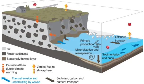
These collapsing Arctic coastlines are not only a potential source for carbon (Lantuit et al., 2009; Tanski et al. 2019) affecting the global carbon stock and can significantly contribute to natural greenhouse gas emissions (Vonk et al., 2012; Wegner et al., 2015), but deliver vast amounts of nutrients (Dunton et al., 2006; Tanski et al., 2016), pollutants such as heavy metals (Fisher et al., 2012; Schuster et al., 2018), and sediments (Obu et al., 2016; Couture et al., 2018) into the sea. While the Arctic is mostly uninhabited, the few coastal settlements and historical sites are widely threatened (Fritz et al., 2017), see also Figure 1-1.
Introduction
2
Figure 1-1. Sketch illustrating the threats and effects on environment and ecosystem along thawing permafrost coasts, from (Fritz et al., 2017).
For inhabitants settlements along the Arctic Ocean, the changes cause large concerns of various nature, as infrastructure and buildings are threatened with arctic coastal erosion rates of up to 20 m/s (Jones et al., 2018), ‘Protecting Tuktoyaktuk from coastal erosion could cost $50M, says mayor’(Zingel, 2019), and adaptation strategies are conflictual,
‘Tuktoyaktuk relocating homes to soon, says resident’ (Last, 2019). Even though, attempts are begone to protect cultural treasure, ‘Gwich’in partner with researcher to map important sites at risk in a shifting landscape’ (Edwards, 2019).
As the Arctic Ocean is losing more and more of its ice, previously hidden resources prompting desires, ‘Unlocking Arctic Energy Is Vital for Alaska and America’ (Murkowski, 2019), ‘Apocalypse Tourism? Cruising the Melting Arctic Ocean’ (Orlinsky & Holland, 2016) opens new possibilities, ’China reveals Arctic ambitions with plan for ‘Polar Silk Road’’ (Wen, 2018) and awakens old conflicts, ‘Arctic Melt Heightens U.S. Rivalry With Russia on the Northern Front’ (Prapuolenis, 2019). While coastal erosion rates are being continuously reported from several arctic coasts, the controlling factors behind the change are not yet completely understood, and accelerating rates urge for insights (Günther et al., 2013; Jones et al., 2018; Irrgang et al., 2018; Lantuit et al., 2011).
Introduction
3
1.2 Objectives
In the Western Canadian Arctic, environmental changes are reported for decades, yet many questions are unanswered. Due to the seasonal ice coverage of the Canadian Beaufort Sea, logistics and long-term measurements are extremely challenging. However, as erosion rates increase (Irrgang et al., 2018), knowledge of the underlain process is needed. The Western Canadian Arctic is known for impressive coastal erosion features like retrogressive thaw slumps are present in the region and are transporting large amounts of material to the sea.
These are ice rich permafrost cliffs, that rapidly erode activated by cliff toe wave erosion, and quickly eroding through melting ground ice that is exposed to warm air temperatures during summer
Figure 1-2. Image of waves approaching Simpson Point in the summer of 2017, a highly threatened shoreline at Herschel Island. In the first decade of the 21. century the erosion rates more than doubled to up to 4 meter per year at this site (Cunliffe et al., 2019; Radosavljevic et al., 2016). Note the historic buildings in the hinterland of the spit. Picture from an AWI time lapse camera – Yukon Coast Summer Expedition 2017.
As the erosional force of approaching waves and the removal of eroded sediment with coastal currents, insights into these acting processes and geometry of the acting hydrodynamics are key for a detailed understanding for the coastal erosion. In order to improve the understanding of coastal erosion, an investigation about the hydrodynamics in the zone near the coast is made. Therefore, measurements of current speed and direction over the course of an arctic field season are performed. The data of these measurements is linked to measured waves and additional available data of environmental forcing parameter.
Scientific Background
4
After data assessing and preparation a linkage of the data is performed, to find implications for the properties of sediment transport in the region and develop ideas for conditions under an emerging Arctic Ocean.
2 Scientific Background
2.1 Arctic Ocean and Sea Ice
The Arctic Ocean is the northern most water body of the planet Earth. Compared to other oceans of the planet, it is a relatively small ocean covering an area of about 15.55 x 10⁶ km2 with an average depth of about 1200 m. With its volume of about 18.75 x 10⁶ km3, the Arctic Ocean contains about 1.4% of the global ocean volume (Eakins & Sharman, 2010). The overall bathymetry is very heterogenous, see Figure 2-1.
Original Scale: 1: 6.000.000 Map projection: Polar Stereographic Standard parallel: 75° N
Horizontal datum: WGS 84
Scientific Background
5
Figure 2-1: Map shows the bathymetry of the Arctic Ocean, adjusted from the International Bathymetric Chart of the Arctic Ocean (IBACO) Bathymetry v3.0 Map (Jakobsson et al., 2012).
The Barents, Kara, Laptev, East Siberian and Chukchi Sea shelf, are extending hundreds of kilometers, with less than 200-meter water depth. They make up about one third of the total size of the Arctic Ocean. In contrast, the Greenland Canadian Archipelago and the Beaufort Sea are relatively narrow shelfs, that transit into deep ocean bathymetry of more than 3000- meter depth in only a little less than 100 kilometres in offshore direction (Williams &
Carmack, 2015). The Central Arctic is characterised by the deep bathymetry of large basins, like the Canada-, Makarov-, Amundsen-, and Nansen basin. That have typical depths of 3000 to 5000 metres, and they are surrounded by underwater plateaus and interrupted by large scale ridges, like the Lomonoso and the Gakkel ridge (Comiso, 2010;
Jakobsson et al., 2012).
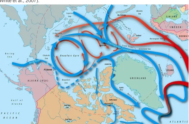
The exchange of water between the Arctic Ocean and other oceans is limited to four gateways: the Bering Strait, the Barent Sea Opening, the Fram Strait and the Davis Strait (Figure 2-2). Additionally, the Arctic Ocean receives vast amounts of fresh, warm and sediment-loaded water inflow from large rivers all over the Arctic (Lammers et al., 2001;
White et al., 2007).
Figure 2-2: Schematic map of major currents of the Arctic Ocean. Map from the website of the Woods Hole Oceanographic Institute (WHOI, 2019).
In consequence of the absence of sunlight, within the polar circle in northern hemispheric winter, the air temperature is extremely cold over the Arctic Ocean. This cold air freezes the
Scientific Background
6
surface water of the Arctic Ocean and forms a mobile layer of sea ice, called pack ice.
Depending of the location of formation it is either transported with the Transpolar Current into the Atlantic Ocean, where it melts within a few seasons, or it gets trapped into the Beaufort Gyre (Figure 2-2), where it may ‘survive’ a melting season and gets older and thicker as multiyear sea ice. In summer, a large portion of the pack ice melts and the ice covered area shrinks drastically.
While the pack ice in the coastal zones of the Arctic Ocean is mobile, sea ice gets attached to the coast (landfast ice) and to the seafloor (bottom fast ice). This locks the coast from freeze up in mid-fall to break up in early summer and largely supresses wave action (Mahoney et al., 2013; Dammann et al., 2019).
Due to the warming of the Arctic in the last decades, the sea ice extent is shrinking, the sea ice thickness is decreasing, the percentage of more stable multiyear ice is declining, and the ice season shortens (Moore et al., 2019). Due to the arctic amplification, that is mostly driven by the decline of sea ice and the resulting decline in albedo, the sea ice loss forms a positive feedback (Serreze & Barry, 2011). A weakened sea ice cover enhances wave action in intensity and duration in the Arctic Ocean, that was previously very limited due to short a fetch and short open water seasons (Overeem et al., 2011; Thomson & Rogers, 2014).
2.2 Permafrost Coasts
The coast of the Arctic Ocean is about 100,000 kilometres long, whereas one-third is classified as lithified and the remaining two-third consists of unconsolidated sediment (Lantuit et al., 2012). Due to the overall extreme cold climatic conditions, sediments are deep-frozen and therefore bounded with ice most of the year. Permafrost is defined as ground, that stayed frozen for more than two consecutive years (French, 2018). In summer, air temperatures far above freezing, lead to an onset of permafrost thaw. Additionally, the open water season in the shelf seas of the Arctic Ocean starts and expose the thawing coasts to erosion.
Along permafrost cliffs two major processes control the erosion, thermo-abrasion and thermo-denudation. Thermo-abrasion occures at the cliff toe, as result of the combination of mechanical action of sea ice and the combined mechanical and thermal action of sea water. Thermo-denudation describes the erosion due to the energy influx on the ground
Scientific Background
7
surface and the resulting thawing of permafrost above the waterline (Günther et al., 2013), see Figure 2-3 for visualization.
Figure 2-3: Image of an exposed permafrost cliff with marked erosional processes of thermo- denudation and thermo-abrasion from Günther et al. (2013).
Additional and special forms of permafrost coastal erosion are retrogressive thaw slumps (Lantuit & Pollard, 2008), active-layer detachment (Lewkowicz, 1991) and, block failure (Hoque & Pollard, 2009) with different extent and importance along the coastline of the Arctic Ocean. The erosion rates of arctic permafrost coasts are in general higher than the rates along other coasts of the world, even though erosion is mainly limited to the summer months, underlining the importance of the thaw processes. Ice keeling of coastal sea ice was considered to add to high erosion rates, yet Aré et al. (2008) found out, that arctic shoreline profiles don’t differ from temperate shorelines, resuming that sea ice plays a minor role in sediment transport and that the wave impact is the major controlling factor. The erosion rate depends on various coastal-, as well as forcing factors. Some of the most important are cliff heights, ice content, orientation, annual air temperature, length of the open water season, fetch length and wave energy. With ongoing climate change, coastal erosion rates accelerate at many sites in the arctic (Irrgang et al., 2018; Jones et al., 2018;
Günther et al., 2015), with extreme average rates of more than 20 m/a (Jones et al., 2018) and are expected to further increase (Barnhart et al., 2014a). Unfortunately incomplete data prevents the analysis of the circum-arctic erosion trend (Overduin et al., 2014; Irrgang et al.
2018).
The sediment mobilised by coastal erosion is often organic-rich (Vonk et al., 2012; Couture et al., 2018) or even contaminated with pollutants (Schuster et al., 2018). Degradation of the organic material can either occure within the erosion features or after transport to the
Scientific Background
8
nearshore water (Vonk et al., 2014, 2015; Tanski et al., 2017, 2019) and is transported offshore or distributed alongshore (Hill et al., 1991). This increase in transported material is considered to alter the ecosystem, as well as the global carbon cycle (Fritz et al., 2017).
Study Area
9
3 Study Area
3.1 Herschel Island and Herschel Basin
Herschel Island - Qikiqtaruk is an island located in the Yukon Territory, Canada. Its centred at 69.5888°N 139.0888°W, about 116 km² in size and approximately 3 km apart from the Yukon Coast in the Canadian Beaufort Sea (Burn, 2012). It has a maximum elevation of 183 m above sea level (Lantuit & Pollard, 2008). The coastline of Herschel Island is defined by a diverse geomorphology. High and steep cliffs are found on the north and west coast at Collison Head and Bell Bluff, with cliff heights up to 50 m. The east coast is less steep, cliff heights range between 20 and 30 m. At the southern coast, cliffs are relatively low and gentle with a height of about 10 m. The southern side boarders towards the Workboat Passage, a shallow and protected embayment. The island has three accumulation features as sand and gravel spits (Obu et al., 2016), that are named Avadlek Spit, Simpson Point and Osborne Point. For site names and locations see Figure 3-1.
Figure 3-1: Map of the official site names along the coast of the Yukon Territory at the Southern Beaufort Sea. Map is from Burn (2012).
The formation of Herschel island results most likely from the latest advance of a side lobe of the Late Wisconsinan Laurentide ice sheet, around 16.200 years ago. This advance resulted in the build-up of an ice-thrust moraine, ridge out of marine sediments that were previously buried and nowadays form the island. The original burial site of these sediments is called Herschel Basin and is nowadays an about 80-meter-deep depression, in the southeast of
Study Area
10
Herschel Island, see bathymetry lines at Figure 3-2 (Lantuit & Pollard, 2008; Rampton, 1982; Fritz et al., 2012).
Herschel Island lies in the continuous permafrost zone with permafrost depths of up to 600 meters (Lantuit & Pollard, 2008). The island is mainly composed of fine-grained, ice-bonded, unconsolidated marine sediments (Pollard, 1990; Fritz et al., 2011). The permafrost here is very ice-rich with an average ice volume between 30% and 60% (Couture & Pollard, 2015;
Fritz et al., 2015; Lantuit et al., 2012a).
The climate is polar continental, with an average annual air temperature of -11.0°C (1971- 2000), while the average July temperature is 7.8°C (1971-2000), measured at the nearby Komakuk Beach weather station (Burn, 2012). A comparison between nowadays temperature at the Herschel Island weather station and records from 1899 to 1905 indicates a climate warming of about 2.5 °C (Burn & Zhang, 2009).
While most studies describe the wind patterns in the Canadian Beaufort Sea region as bimodal with dominant north-western winds and subordinated easterly winds (Solomon, 2005; Radosavljevic et al., 2016; Burn, 2012), Hill et al. (1991) highlighted southwest wind as a third major wind direction at the Yukon Coast. These winds are associated with mountain barrier baroclinity and the orographic effects of the nearby Brooks Range (Kozo
& Robe, 1986), while the bimodal winds are generated around large scale pressure systems in the Beaufort Sea. In general, the wind pattern seems to vary largely from year to year (Fissel & Birch, 1984 as cited in Hill et al., 1991), but recent studies suggest a shift towards more easterly winds (Wood et al., 2013; Wang et al., 2015). In summer, wind speeds are moderate to high with maximum reported wind speeds of 18.6 m/s NW and 12.8 m/s E (Radosavljevic et al., 2016), 11.1 m/s NW and E (Cunliffe et al., 2019), and SW winds of up to 20 m/s (Hill et al., 1991). Storms occurring mostly in fall (Solomon, 2005).
Positive storm surges in the region are associated with a south-eastward water push onto the coast by north-westerly storms. The storm surges can produce a local water level up- set of up to 2.4 m at favourable sites in the Southern Beaufort Sea, but are likely less extreme around Herschel Island (Forbes & Frobel, 1988; Harper, 1988; Hill et al., 1991; Pelletier &
Medioli, 2014).
Herschel Island lies within the Canadian Beaufort Sea, a marginal sea of the Arctic Ocean, that is characterised by its steep margin and relatively narrow shelf (William & Carmack, 2015). The Canadian Beaufort Sea coast is considered as wave dominated and microtidal, with an astronomical tide ranging from 0.3 meter to 0.5 meter (Héquette et al., 1991).
Typically, the Beaufort Sea is frozen for eight months of the year, with a freeze-up in October and break-up in June. In the winter season the ice is largely blocking ocean-atmosphere
Study Area
11
exchange and wave action. The coastal zone up to the 20 m isobath is then occupied by landfast and bottom fast ice (Mahoney et al., 2013; Carmack & Macdonald, 2002). Ongoing climate warming elongates the ice-free season by more than nine days per decade in the Beaufort Sea (Stroeve et al., 2014). Around Herschel Island rates are even faster, with reported shift of 15 days per decade recently (Barnhart et al., 2014a).
In early summer the combined force of sun radiation and warm water of the Mackenzie River forces the ice to melt and pushes it offshore out of the delta (Dunton et al., 2006). The Mackenzie River is the fourth largest of the big arctic rivers. It has an annual discharge of 316 cubic kilometre per year and considering the size of the shelf, it is the most impactful river of all arctic rivers (Carmack et al., 2015). It provides vast amounts of sediment, warm and fresh water into the Canadian Beaufort Sea and dominates as sediment source (Hill et al., 1991). In summer under east wind conditions, the Mackenzie River plume spreads towards the coastal part of Herschel Island.
When in summer the sea ice retreats, the fetch can get hundreds of kilometres large, occasionally up to 1000 kilometre in recent years (Thomson & Rogers, 2014). In this large open water area, waves up to five meter can be generated under storm conditions in the central part of the Beaufort Sea (Thomson & Rogers, 2014). For the region close to Herschel Island the mean significant wave heights are 0.45 meter to 0.6 meter in July and August, while ranging between 0.9 meter to 1.05 meter in September (1992-2013) (Wang et al., 2015, based on the MSC Beaufort Reanalysis; Swail et al., 2007). Additionally, Wang et al.
(2015) showed an increase of significant wave height of about 0.5 % per year (1971-2013), likely due to increased fetch. In-situ measurements of waves in coastal waters are very rare in the western Canadian Beaufort Sea. A study within a two-week period in late summer 1985 near King Point (circa 40 kilometer southeastward of Herschel Island), recorded moderate wave heights up to 0.8 meter (Hill et al., 1991).
The largest current around the Beaufort Sea is the Beaufort Gyre. It flows in westward direction bordering between the Arctic Ocean and the Beaufort Sea shelf. Contrary to this, at the continental slope, the Beaufort Undercurrent is flowing towards the east. On an occasional base, it provides its nutrient-rich water. It is delivered upon the shelf by upwelling events or through Canyons, like the Mackenzie Canyon, around 50 kilometer north of Herschel Island. The flow is considered to mainly wind-driven and variable with speed up to 0.5 m/s in summer, and less than 0.05 m/s in winter (Dunton et al., 2006; Forest et al., 2016).
In the nearshore zone of the Canadian Beaufort Sea, currents are not well studied. The knowledge is gained from a few studies in the Eastern Part of the Canadian Beaufort Sea
Study Area
12
and a study at King Point (Davidson et al., 1988; Hill et al., 1991; Hequette et al., 1993). In general, most currents in the coastal zone are wind driven, with an impact of waves depending on site and water depth. A decreasing trend in current strength seaward and down from the water surface. Small scale topography and coastal setting have an impact as well.
The flow speeds range up to 0.5 m/s at the bottom are in general between 0.1 and 0.2 m/s.
The direction of flow is highly diverse depending on wind direction, direction of wave approach and up- and downwelling events. Around Herschel Island, Pelletier & Medioli (2014) located the main sediment drifts mainly based of knowledge about dynamical features along the coast, see Figure 3-2.
Figure 3-2: Map of Coastal Landforms and Processes around Herschel Island modified from (Pelletier & Medioli, 2014). The mooring sites of 2015 and 2018 are marked as asterisk.
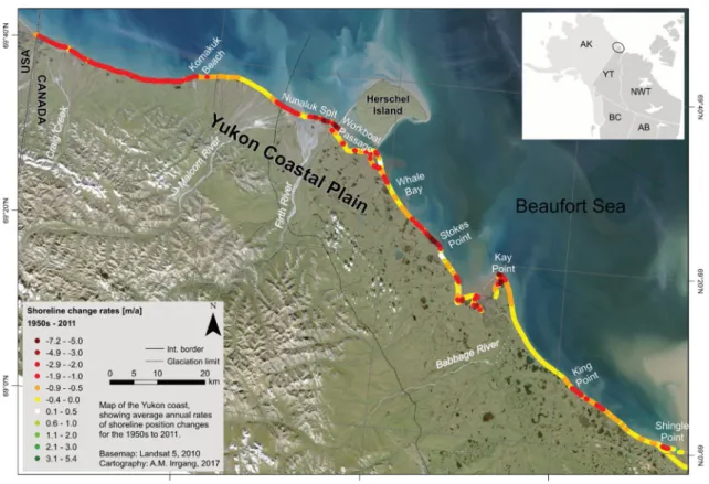
The combination of wave action, currents and thawing in the summer season rapidly erodes the coast along the Yukon Coast and the Mackenzie delta. In the Mackenzie delta erosion rates of up to 22.5 meter per year are measured, with an average rate of 0.6 meter per year (1972-2000) (Solomon, 2005). At the Yukon Coast latest average erosion rates are 1.3 meter per year with locally up to 8.7 meter per year (Irrgang et al., 2018), see Figure 3-2.
Study Area
13
At Herschel Island latest average erosion rates are 0.68 meter per year (2000-2011), see Figure 3-3 and show a general increasing trend regarding previous decades (Obu et al., 2016; Lantuit & Pollard, 2008). Cunliffe et al. (2019) showed, that erosion can be highly episodic (hours to days) in the region and short strong wind events can account for large portions of the annual erosion rate.
Figure 3-3: Shoreline change rates (1950-2011) along the Yukon Coast, Canada. Map from Irrgang et al. (2018).
The geomorphologic erosion processes in the region include active layer detachment, cliff incising, block failure and retrogressive thaw slumps. The later are known to transport large amounts of sediment, nutrients and carbon into the nearshore waters (Ramage et al., 2018;
Tanski et al., 2017). Couture et al. (2018) show an annual flux of 36 x 106 kilogram of carbon for the Yukon Coast.
3.2 Location A – 2015 – Simpson Point
The first study site is in the eastern part of Qikiqtaruk, Herschel Island next to Simpson Point.
Simpson Point is the location of a historic whaling settlement, it has many archaeological sites, see Burn (2012). It is a spit mostly composed of sand and gravel. It is about 870- meter-long and has a mean elevation of 0.35 m with maximum heights of 1.2 m, see Figure 3-4. Due to its low elevation the spit and the historic sites and buildings are prone to flooding and threatened by the global sea level rise (Radosavljevic et al., 2016).
Study Area
14
Simpson Point is attached to an alluvial fan a bit further northeast, that comprised of redeposited marine and glaciogenic sediments. The coastline of this nearby fan consists out of one- to five-meter-high ice-rich bluffs, that erode very fast (Radosavljevic et al., 2016;
Cunliffe et al., 2019). The eroded sediment of the retreating fan and the eroded material from the 30-meter-high cliffs of Collison Head towards the northeast are supplying Simpson Point with sediment (Obu et al., 2016; Radosavljevic et al. 2016).
Figure 3-4: Site photography of Simpson Point, photographer (author) stands on top of Slump D, a retrogressive thaw slump at the eastern site of Herschel Island and views towards the east. Scene is from early August 2018. Low lying spit, Simpson Point at the right-hand site, alluvial fan to the left, high cliffs of Collison Head behind. Note the high amounts of sea ice in the Pauline Cove and further offshore in the Southern Canadian Beaufort Sea.
The orientation of the spit is east west, with a natural protection against waves towards the north, the west and a short fetch of less than 20 kilometers towards the south. This orientation leaves the spit only directly exposed to waves approaching from the northeast to southeast. Even under these protected conditions, most of the seaward coastline of the spit is retreating with accelerating rates, of up to 5.5 meter per year (2000-2011), while the landward site towards Pauline Cove is highly dynamic and partly advancing. Overall Simpson Point is threatened by the potential of erosion, the often-occurring floods and the
Study Area
15
global sea level rise (Radosavljevic et al., 2016), see Figure 3-5 for illustration of the trend in shoreline movement.
Figure 3-5: Shoreline change rates at the eastern most part of Herschel Island (1952-2011). This map is from Radosavljevic et al. (2016) and highlights the varying shoreline change rates along different coastal transects. Note the deeply incised cliffs of Collison Head at the right, the alluvial fan with its high erosion rates in the left-hand site and the highly dynamic spit Simpson Point in the lower left corner of this map.
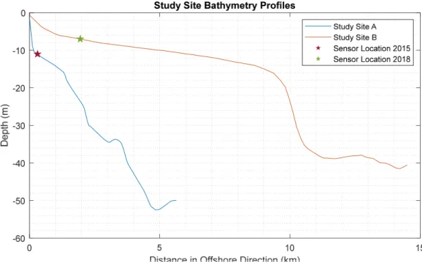
The transition from the coast towards the northwestern site of the Herschel Basin is relatively steep. Nearshore zone (up to 20 meter water depth) is up to about 1.5 kilometer from the coast, while the deepest parts of Herschel Basin are around eight kilometer in offshore distance, see Figure 3-8. This indicated the short transport ways for sediment towards the basin and back.
3.3 Location B – 2018 – Catton Point
The second study site named Catton Point or Calton Point, is a five-kilometer-long and 20 to 50 meter wide recurved spit. It separates the Ptarmigan Bay, a shallow lagoon, from the Southern Canadian Beaufort Sea. The spit is striking NNW -SSE and therefore exposed to open water conditions from northeast to southeast (Burn, 2012; Hill et al., 1991).
Study Area
16
On this gravelly spit, several traditional hunting and historical sites are located. According to Irrgang et al. (2019), 30 historical features are presented along the spit and seven more at the Ptarmigan Bay. In the central part of the lagoon lies a large relict island with up to five- meter-high bluffs that is boarded towards the inner site of the spit (Hill et al. 1991), see Figure 3-6.
Figure 3-6: Site photography from helicopter towards the southeast. Note the central island in the inner part of the lagoon and the large amount of aligned driftwood logs on the spit. At the right-hand site lies the shallow Ptarmigan Bay lagoon, on the left-hand site Southern Canadian Beaufort Sea.
Picture by Goncalo Viera in 2018.
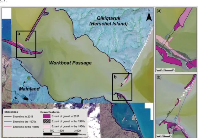
Catton Point builds the southeastern entrance to the Workboat Passage, south of Herschel Island, see Figure 3-7. The Catton Point spit is highly dynamic. A geographic map from 1890 of the area around Herschel Island shows two unconnected barrier islands at the position of nowadays Catton Point, see Appendix B. Irrgang et al. (2019) illustrate its highly dynamic
Study Area
17
movement in the last decades (1950-2011) with the usage of satellite imagery, see Figure 3.7.
Figure 3-7: Map of dynamic movement of coastal features at the southern end of Herschel Island with a focus on the western and eastern entrance to the Workboat Passage. The lower right-hand site image shows the advance of the Catton Point spit towards the Workboat Passage. This map is from Irrgang et al. (2019).
Shoreline change rates (1950 to 2011) along the Catton Point spit are variable, according to data from Irrgang et al. (2018). The shorelines of the distal part and the proximal parts are retreating with rates up to 1.9 m/a, while the central part around the relict island is stable.
The tip of Catton Point is rapidly moving towards the Workboat Passage, with an advance of about 500 m in 61 years (average annual rate of 8.2 m/a), based on Figure 3-7. The supplied sediment probably originates from eroding coasts in downdrift (southeast) direction Irrgang et al. (2018).
The slope from the shoreline of the spit towards the Canadian Beaufort Sea is gentle up to about nine kilometers offshore (15 m water depth), where it steepens towards the central part of Herschel Basin, see Figure 3-8 and 3-9.
Study Area
18
Figure 3-8: Bathymetry profiles approximately perpendicular from the coastline towards the mooring sites and into the basin. Note the difference in slope gradients between the two measurement sites. Profiles were extracted from the bathymetry model below with usage of the TopoToolbox 2 (Schwanghart & Scherler, 2014), uncertainties arise from the limited accuracy of bathymetry data, and the interpolation.
Figure 3-9: Bathymetric model of Herschel Basin. The model is based on bathymetry data from O’Connor (1984), that were digitized by Hugues Lantuit in ESRI ArcMap (ESRI, 2019). In MATLAB, processing and graphic design for this thesis was performed by the author. The bathymetry lines are at 2, 4, 6, 8, 10, 15, 20, 30, 40, 50,60, 70, and 80-meter depth. Refer to the legend of the graphic for symbols. Note the exaggeration and the misleading position of the red start due to an inaccurate resolution at Simpson Point.
Methods
19
4 Methods
This thesis aims to study the influence of environmental forcing factors on currents in the nearshore zone of the study area. Therefore, a current measurement device (ADCP) was mounted at the seafloor in two separate years and related environmental data were obtained, to link the forcing of wind, fetch, waves and stratification on the behaviour of currents at this location.
The first part deals with the acquisition and processing of the in-situ data with moored instruments, publicly available environmental data and modelling products of the study location A – Simpson Point in the year 2015. The mooring started at the 27th of July 2015 at 22:45 and ended at the 14th of August 2015 at 14:15 and was not performed by the author, but by the expedition team of the Yukon Coast 2015 summer expedition.
The second part deals with the acquisition and processing of the in-situ data with moored instruments, publicly available environmental data and modelling products of the study location B - Catton Point in the year 2018. The mooring started at the 4th of August 2018 at 0:00 and ended at the 18th of August 2018 12:00.
For exact and uniform processing and presentation of the data, all data was imported into MATLAB and further analysis and visualisations were performed.
4.1 Measurement Methods Study Location A – 2015 4.1.1 Wind
Wind data was obtained from the nearest official World Meteorological Organisation weather station, due to a failure at the weather station at Herschel Island during the mooring period, the data of the second nearest is taken, which is the Komakuk Beach weather station. This station is listed as number 71046 at the World Meteorological Organisation and roughly 50 kilometer westward of the mooring site (Environment Canada, 2019). This weather station measures air temperature, wind speed, wind direction, dew point temperature, relative humidity and air pressure every minute and averages the data to hourly values. The data was downloaded in XML-format at http://climate.weather.gc.ca. For further processing the hourly wind speed and direction values within the mooring period were extracted and stored in a MATLAB timetable, then the data was averaged into three-hourly mean values for further analyses. The resolution for wind direction is 10 degree and the resolution for wind speed is one kilometer per hour (0.28 m/s).
Methods
20
4.1.2 Sea Ice – Directional Fetch
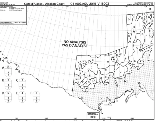
The concentration of sea ice and the position of the ice edge was obtained using the daily sea ice data from the Canadian Ice Service (CIS, 2005). Daily sea ice charts are available for the western arctic from 1999 on and cover the season from mid June to end of October of each year. They are publicly accessible under the website of Environment and Climate Change Canada (CIS, 2019) and were previously used for other studies of sea ice in the Canadian Arctic (Manson et al., 2016). The product is delivered in gif-format. Every chart contains a geographic coordinate system as grid, sea ice data in form of the international EGG code and an information box about the used sensors to produce the chart. The charts are standardized, containing the same grid and are filled with ice information of available sources, various radar satellites imagery and icebreaker data in the region. They are updated till 18:00 at the specific date.
In the mooring period of 2015, every chart was at least produced with the help of RADARSAT or even higher resolution products. The estimated accuracy of the ice edge position for a 100m resolution imagery, like RADARSAT is given 630 meters (CIS, 2005).
The charts in the mooring period are downloaded and loaded into MATLAB, where the data format was changed from gif to tif (tagged image format). The unprojected charts were imported into ArcMap, where the graticules of the charts were used for georeferencing.
Therefore 15 widely distributed grid cross points, spanning the whole area, were used to act as reference points for a 2nd order polynomial transformation.
The georeferenced maps were used to draw a shapeline on the edge of the sea ice to determine the open water area around the moored sensor. The edge was defined as boundary between open water and areas with more or equal than 20 % sea ice concentration, while the resolution of the sea ice concentration of the charts is 10%. In using 20 % as threshold concentration, this study orientated at previous studies that used 15%
sea ice concentration as threshold (Overeem et al., 2011; Barnhart et al., 2014a). This is a conservative approach, as other studies used higher sea ice concentrations as determination for areas of no wave propagation (Swail et al., 2007). Even though, Barnhart et al. (2014a) considered this simple approach as enough. Other studies showed that the sea ice concentration as the only input is a simplification and showed that other ice
Methods
21
properties like thickness and flow size diameter play significant roles in their wave dampening effects. (Manson et al., 2015; Zhang et al., 2015).
Figure 4-1: Paradigm chart of sea ice product of the Canadian Ice Service (CIS, 2019)
The position of the sea ice edge was mapped starting at the closest sea ice feature to the west and goes on along the ice edge clockwise to the east, until land was reached.
The produced daily sea ice edge shapelines were imported into MATLAB, where they were used together with shoreline data of the GSHHG dataset (global self-consistent hierarchical high-resolution shoreline) (Wessel and Smith, 1996) to determine the distance from the sensor to the nearest sea ice edge or land feature. Therefore, an algorithm was programmed in MATLAB, starting with the position of the sensor, the sea ice edge line of the respective day and the shoreline. It computes, angle preserving lines from the sensor position in each direction and finds the intersection points of the line and the sea ice edge or coastal feature.
The closest point is chosen and the distance from the sensor to this point is calculated. The
Methods
22
results are the distances in kilometers to the ice edge or coast at every specific day from 10 to 360 degree in ten-degree increments.
Figure 4-2: Example of the determination of fetch length for a day, here the 6th of August 2015. In MATLAB, the sensor location (red triangle) is used as starting point to determine in every direction (yellow lines) (ten-degree increments) how far the next shoreline (red line) (GSHHG dataset) (Wessel
& Smith, 1996) or edge of same or greater than 20% sea ice concentration (light blue broken line) (CIS, 2019), that was mapped before in ArcMap using daily charts of the Canadian Ice Service is (CIS, 2005).
To determine how much distance for wave generation at a specific time was available, the so-called directional fetch was calculated, an approach introduced by Overeem et al.
(2011). The hourly wind direction is taken (Chapter 4.1.1) and in the direction the wind was blowing from, the distance to the sea ice (daily updated boundaries) or land from the sensor was defined as fetch at this time. Afterwards the hourly values for the directional fetch were average to three-hourly values.
4.1.3 Modelled Waves
In 2015, the mooring had no instrument for the measurement of waves. To overcome this gap, several options were considered. The best cast would have been measurements of wave height, using buoy data or satellite measurements. Unfortunately, both are unsuitable for this study. Publicly available satellite data in the study area has a poor temporal resolution of about two weeks, which is highly unsatisfying for measurements of wave heights over a short field season. Data from wave buoys, which are widely used for wave measurements in all regions of the world, are not available in the Canadian Beaufort Sea. The closest buoy
Latitude
Methods
23
to the study site is in offshore waters of the US American Beaufort Sea (National Data Buoy Center, 2019) and are to far away to represent the local waves.
To overcome this gap in direct measured wave properties, available hindcast data are used.
The most famous wave hindcast for the Canadian Beaufort Sea is the commercial MSC Beaufort Reanalysis (Swail et al., 2007), that is produced every few years. But unfortunately, they did not produce available data in the study periods. Instead, the NOAA WaveWatch III® (NWW3) multigrid productional hindcast was used (Tolman, 2008; WW3DG, 2016). This hindcast uses all available data, such as daily ice fields and hourly wind data to calculate wave parameter globally in different grids, while each grid can influence each other (Chawla et al., 2013). For further information and the possibility to access the hindcast data the reader is referred to the website of the Environmental Modeling Center (EMC, 2019) Fortunately, the grid for the coastal waters of Alaska is large enough to cover our study area in the Canadian Beaufort Sea. For the Alaskan coastal waters, the grid resolution is four arc minutes: This is a much higher spatial resolution than the Arctic Analysis and Forecast by the Copernicus service of the European Union has. They use the WAM model (WAMDI Group, 1988; Saetra et al., 2018).
The NWW3 model is occasionally updated and refined. Unfortunately, one of the major updates fell into the mooring period of 2015 (WW3DG, 2016). In order to keep the data comparable within the dataset, as well as with the data from 2018, only wave data after the update is considered. The data calculation changed with the 1st of August 2015 0:00 UTC, which is equivalent to the 31st of July 2015 18:00 at the study site.
The data output has a temporal resolution of three hours and is provided in grib2-format. To simplify the data processing in MATLAB the data was converted into NC file format, using the Netcdf-Java ToolBox from Signell & Bhate (2013) to process the data. The grid point that is nearest to the mooring location is 69.533 °N 138.867°W. Using this grid point, the time-series of wave direction (resolution of 0.01 degree) and significant wave height are obtained (resolution 0.01 m). See Chapter 4.2.4 for further explanation of this parameter. In MATLAB further processing and graphical analysis were performed.
4.1.4 Stratification
To investigate on the layering of the water column, the stratification was measured occasionally near the moored sensor using a handheld CTD probe. The device used was a CastAway® CTD that was lowered from a small boat. The instrument records the position in the water column, the conductivity and temperature at that position. While temperature is
Methods
24
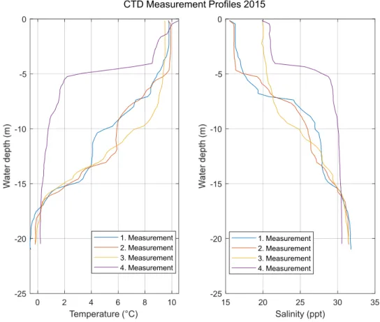
measured directly, the device calculates salinity from measured conductivity. The data is initially stored on the device and can be downloaded afterwards with the associated CastAway® CTD software (Xylem Inc., 2012). The datapoints of interest were selected and exported to MATLAB. In MATLAB data was analysed using basic statistical parameter and was prepared for display.
4.1.5 Currents
The main goal of this thesis is to measure and analyse the currents of the study area in direction and speed.
Various techniques for the measurement of currents are available. Methodical approaches that track the position of a passively flowing drifter over time are known as Lagrangian Method (Joseph, 2014). It provides speed and direction of a flow over a wide area along the path but it is limited in time and more useful to obtain the flow structure over a large area (up to hundreds of km). Techniques that measure the currents stationary, to create time- series of flow velocity and direction, are called Eulerian approaches (Joseph, 2014). It provides a detailed stationary long-term current record throughout the water column and is widely used in coastal engineering and environmental assessments (Joseph 2014).
One device that uses the Eulerian measurement approach is the so-called Acoustic Doppler Current Profiler (ADCP). The ADCP emits acoustic pulses through their beams at a certain frequency through the water column and measures the backscattered doppler-shifted acoustic signal in various predefined depth cells (bins). The pulses get backscattered at particles that drift passively in the water with the speed and in the direction of the water.
Signals of actively moving objects like fish are removed in the post-processing to prevent signal errors (Gordon, 1996; Terrey et al., 1999a; Joseph, 2014).
The device used for the study was an RDI Teledyne Workhorse Sentinel 600 kHz ADCP (Teledyne RD Instruments Inc. 2001, 2008). It has four beams that are 20 degree tilted, forming a so-called Janus configuration. The 600kHz stands for the frequency in which the pulses are emitted, different pulse frequencies have different properties in maximum range and resolution (Teledyne RD Instruments Inc., 2008)
Prior to the mooring, the device was calibrated at the field site, following the standard steps of the user guide (Teledyne RD Instruments Inc., 2001), by using the set-up software RD Instrument WinSc (Teledyne RD Instruments Inc., 2001). This includes a beam check, clock check and compass calibration, which is an important step to perform onsite, as magnetic field varies global. Due to the relative proximity to the north pole magnetic field variations
Methods
25
can be rather big (Hamilton, 2001). After calibration and check ups, the measurement properties were configurated. The depth cell was set to 0.50 meter, being a compromise of a small cell size with a relatively large error and a large bin size, with smaller error but less resolution (Teledyne RD Instruments Inc., 2008). The number of cells (bins) was set to 29.
The first bin starts at 1.59 meter, which is the first technical possible height above the seafloor to measure, so that potentially a water column of 15.59 meter could be measured.
As bathymetry is not completely known in the area the position of the mooring platform, this was to make sure a potential deeper site could also be covered.
The measurement cycle was put to 15 minutes, as a compromise between battery lifetime and coverage. The device works in a way, where in every cycle 50 pulses, so-called pings in equal spacing are emitted, being here a ping every 18 seconds. This ensemble measurement is used to reduce the standard deviation value, which is 12.9 cm/s for a single ping at 0.50-meter bin size by device design. Using an ensemble measurement of 50 pings reduces the standard deviation value to 1.8 cm/s, calculated with the following formula from (Joseph, 2014, p. 342), where σVmean is the standard deviation for the speed of an ensemble measurement, σVping the standard deviation of the speed for a single ping measurement and
√ the square root of the number of pings that are ensembled.
After the pre-deployment software set-up was done, the device was mounted on a steel platform, equipped with a weight and a buoy for platform retrieve and was then lowered from a small boat. The weight keeps the buoy in place next to the platform but a bit off to avoid buoy induced movements to affect the measurements. The platform was mounted at 69.558393°N 138.914445°W in eleven-meter water depth or so, varying with sea level (Figure 3-2 and 3-9) and started recording at the 27th of July 2015 22:45.
At the 14th of August 2015 at 14:15, the platform was retrieved, the data was downloaded from the device and stored. Later imported into RDI Velocity, which is the latest postprocessing software of the Teledyne RD Instruments Inc. (Teledyne RD Instruments Inc., 2018). Using this software, the first step is to calibrate the measurements by determining the salinity. Here 20 ppt was used as compromise between less saline waters of the Mackenzie river plume and the more saline water of the arctic ocean (Mulligan et al., 2010). For density, the standard value was used. For the calculation of the speed of sound the recalculation option of the software was used, that calculates the speed of sound using
Methods
26
temperature, salinity and depth. The value for magnetic declination (22.45°) was obtained from the National Geophysical Data Center for the mooring period and study site (NGDC, 2019).
The "Range to boundary - Intensity" function of the Velocity software was used to remove bins that were affected by turbulent mixing of air particles. The software uses the backscatter intensity for this sorting (Teledyne RD Instruments Inc., 2018). Afterwards the dataset was exported into MAT-file format and then loaded into MATLAB. In MATLAB the data was averaged into three-hourly values, as standard measurement period here for the different environmental parameter. The bins were merged into bottom (1.59 meter above the seafloor to 2.59 above the seafloor), upper water column (9.59 meter above the seafloor to 10.59 meter above the seafloor) and the 14 bins in between (2.59 meter above the seafloor to 9.59 meter above the seafloor) as mid column. The differing column size are used to preserve the signal near the sea surface (upper column) and near the seafloor (bottom column), while using two bins each to prevent potential bin specific errors to falsify the data. The final step was the visualisation of the data in MATLAB (Berens, 2009).
4.2 Measurement Methods Study Location B -2018
The in-situ measurements in 2018 were performed by the author with the help of the team of the Yukon Coast 2018 summer expedition.
4.2.1 Wind
For the study in 2018, the wind data was obtained using the nearest official weather station, which was the Herschel Island Weather Station (WMO Identifier: 71501) (Environment Canada, 2019). The data handling was done like in 2015, explained in Chapter 4.1.1.
4.2.2 Sea Ice – Directional Fetch
The methodical approach and implementation are the same as in the 2015 data period, described in Chapter 4.1.2.
Methods
27
4.2.3 Modelled Waves
The methodical approach and implementation are the same as in the 2015 study, see Chapter 4.1.3., different only in the grid point of data extraction and the period. In 2018, the nearest data point to the sensor location was at 69.4666°N and 139.0001°W.
4.2.4 In-Situ Waves
In Contrast to 2015, the mooring platform had a sensor for measurement of wave height.
The logger model was the RBR solo³ D |wave16 (Tsai et al., 2005; RBR Ltd., 2017) which is a nondirectional pressure sensor. It measures the water pressure in a high frequency to reveal fluctuations of the surface. The logger was pre calibrated for up to 20-meter water depth. Prior to deployment the device was configurated using the manufacturers standard software RBR Ruskin, where different measurement profiles are available (RBR Ltd., 2019).
The sensor was configurated for the burst mode, where it measures every five minutes 4096 times with a frequency of 16 Hertz (RBR Ltd., 2017, 2018a).
After the set-up, the device was mounted on the ADCP, sitting 0.1 meter above the seafloor.
The data was retrieved from the sensor using the RBR Ruskin software, that automatically imports the raw data and calculates wave statistics for the recorded pressure signal (RBR Ltd., 2019). For further analysis the datafile was exported to MATLAB, where a specialised MATLAB Toolbox (RSK MATLAB Toolbox Version 3.1.0) simplifies the work with the dataset (RBR Ltd., 2018b). To separate the measured water pressure from the total pressure (air pressure and water pressure), the raw data was corrected in MATLAB using pressure data that was recorded in a nearby field site at 69.57743°N 138.90130°W (Coch et al., 2018).
The used sensor was a HOBO U20 Water Level logger (Onset, 2012). It recorded air pressure every hour, this dataset was exported into MATLAB, where a spline interpolation was performed to resample the data to a five-minute interval. The calculations that are performed in order to transfer the pressure signal to wave statistics can be found in (RBR Ltd., 2018b). The wave parameter that is of most importance for this study is the significant wave height (SWH), which is equal to the average wave height of the highest one-third of all measured waves. This parameter is widely used, when working with wave heights (Francis et al., 2011; Barnhart et al., 2014a). In MATLAB further data statistics and figure preparation was performed.
Methods
28
4.2.5 In-Situ Sea Level
The sensor described in Chapter 4.2.4 does not only measure the water pressure changes occurring from waves, but also pressure change from water level fluctuations like tides and surges. The data of water level above the sensor is used to determine the sea level at the mooring site. The data is displayed in MATLAB.
4.2.6 Stratification
The methodical approach and implementation are the same as in the 2015 study.
4.2.7 Currents
While the methodical approach and the device are the same as in the 2015 study, the implementation is slightly different. The measurement frequency was enhanced, that the sensor took data every minute, ping every 1.2 seconds, instead of every 15 minutes, ping every 18 seconds. The study site was further southeastward at a gentler slope and a shallower site, deployment depth of seven meter. The location was at 69.465833°N 139.030555°W, the mooring started at the 4th of August 2018 0:00 and ended at the 18th of August 2018 12:00. Due to the change in location the magnetic declination value for this site and time period was 20.26°, obtained using the same way as in Chapter 4.1.5.
Due to the shallower depth, the number of bins decreased, so after removing of the topmost bins, see Chapter 4.1.5, the lowest two bins were used as bottom (1.59m above the seafloor to 2.58 meter above the seafloor), the upmost two were used as upper water column (4.59m to 5.59m above the seafloor) and the four bins (2.59m to 4.59m above the seafloor) in between were used as mid water column.
Results
29
5 Results
The result section is following the methodical structure of this thesis and separates the 2015 data set near Simpson Point from the 2018 data set near Catton point. The first study started at the 28th of July 2015 0:00 and ended at the 13th of August 2015 15:00, the results of this are shown in part 5.1. The second study period spans from the 4th of August 2018 0:00 to the 18th of August 2018 15:00, the results of this are shown in part 5.2.
In the third and fourth part of this chapter, a simple statistical analysis is presented, to investigate on the linkage between environmental forcing parameter and the response of the currents, again separated by years.
5.1 Results for Study Location A – Simpson Point 2015 5.1.1 Wind
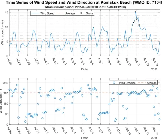
The measurement period for the 2015 mooring started at 28th of July 2015 0:00 and ended on the 13th of August 2015 15:00. The maximum wind speed was 15.3 m/s (55.1 km/h) at 10th of August 2015 21:00, minimum wind speed occurred at 13th of August 2015 6:00 0.6 m/s (2.2 km/h). The mean value for the wind speed is 5.3 m/s (19.1 km/h), the median value 4.7 m/s (16.7 km/h) and standard deviation value is 3.0 m/s (10.8 km/h).
One arctic storm event, following the arctic storm definition of Atkinson (2005), where an arctic storm is a period of at least 6 hours with wind speeds of at least 10 m/s, occurred.
The storm started at the 10th of August 2015 at 12:00 and ended at the 11th of August 2015 at 06:00, the wind was coming from west, with wind directions between 260 degree and 280 degree. The wind speed varied from 10.6 to 15.3 m/s (38.2 km/h to 55.1km/h). The time series of wind measurements in 2015 is visualised in Figure 5-1.
The wind direction in the measurement period varied from 27 degree to 340 degree (clockwise). The wind data is presented, following the meteorological convention, where the direction indicates the origin of the wind (Thomson & Emery, 2014). NE to SE winds had varying wind speeds, wind from SE to SW had only low wind speeds, while winds from SW to NW had varying speed. Additionally, a very few winds were recorded from N. In Figure the 5-2, the distribution of wind in the 2015 measuring period is illustrated in a polar scatter plot.