M. Stiemer1, M. Klocke2, F. T. Suttmeier1, H. Blum1, A. Joswig2, S.
Kulig2
1Chair of Scientific Computing, University of Dortmund
2Institute of Electrical Machines, Drivers and Power Electronics, University of Dortmund
Abstract
Electromagnetic forming (EF) is a high speed forming process in which strain rates of over103 s−1are achieved. The workpiece is deformed by the Lorentz force resulting from the interac- tion of a fast varying electro magnetic field with the eddy currents induced by the field in the workpiece. Within a research group (FOR 443) funded by the German Research Foundation (DFG) an object oriented simulation tool for this multi physical process has been developed (SOFAR), that can handle the fully coupled simulation in a single software environment. In this contribution, details of the algorithmic implementation of the electromagnetic side of the coupled model are discussed and validated. Basis of this validation are benchmark simulations developed for this purpose. In particular, the implementation of transient field computation for coupled problems within SOFAR is compared with an experienced FD-code (FELMEC) devel- oped at the Institute of Electrical Machines, Drives and Power Electronics.
Keywords:
Modeling, Simulation, Electromagnetic Forming
1 Introduction
Electromagnetic forming (EF) is a dynamical forming process that is driven by the interaction of a pulsed magnetic field with eddy currents induced by the exciting field. The workpiece to be formed consists of good conducting material like copper or aluminum. A tool coil adjacent to the workpiece is excited by a fast time varying current. The resulting pulsed magnetic field diffuses into the work piece and induces eddy currents there. These eddy currents again in-
*This work is based on the results of the research group FOR 443. The authors wish to thank the Deutsche Forschungsgemeinschaft – DFG for its financial support.
teract with the exciting magnetic field which results in a material body force, e.g. the Lorentz force representing an additional supply of momentum that results in deformation. EF offers advantages over other forming methods such as increase in formability for certain kinds of ma- terials, reduction in wrinkling, the ability to combine forming and assembly operations, reduced tool making costs etc.. Despite these advantages, its industrial application is concentrated on joining tubular semifinished material (see [1, 2]), whereas electromagnetic sheet metal forming (ESF) has not been developed to a point where it may be routinely used for industrial purposes yet. The determination of the optimal progression of the magnetic field strength including the design of tool coils and power supply devices requires still scientific research. Nevertheless, recent research activities [3, 4] have led to a precise description and process analysis of the free forming of aluminum sheet metal.
The above mentioned difficulties demonstrate the significance of reliable simulation tools for EF. However, these require a non linear coupling of a mechanical simulation considering the material’s dependence on the strain rate with an electromagnetical one. Since the introduction of high speed computers in the late 80’s, several different approaches to EF have been carried out (see [5, 6, 7, 8, 1, 2, 3, 9]). The simulation developed within the DFG research group FOR 443 is based on a general approach to the formulation of continuum thermodynamic models for a class of rate-dependent metallic engineering materials dynamically formed via strong mag- netic fields due to Svendsen and Chanda [10, 11]. The validity of (a specialised form of) these models has been verified experimentally in Brosius et al. [12, 13]. The algorithmic formula- tion of the coupled model and its efficient numerical implementation has been carried out and discussed in [14]. As software environment the object oriented code SOFAR (SmallObject ori- entatedFinite-element-library forApplication andResearch) has been chosen [15]. Moreover, the mechanical side of the simulation has been validated by benchmark simulations in [16].
In the present contribution we discuss different algorithmic approaches to the model- ing of the electromagnetic subsystem of the coupled process and report on its validation by a benchmark procedure. It is analysed which numerical techniques are best suited to solve certain problems arising in the simulation. In particular, the algorithmic implementation within SOFAR is compared to a well experienced FD-code (FELMEC) developed and maintained at the Institute of Electrical Machines, Drivers and Power Electronics. In addition, results from experiments carried out at the chair of forming at the university of Dortmund by Badelt et al. [3]
and Beerwald et al. [4] serve as references.
2 Model Formulation of the Electromagnetic Subsystem
2.1 Derivation of Basic Equations
The state of an electrodynamic system is characterized by for vector fieldsE,~ D,~ B~,H, fulfilling~ Maxwell’s equations
divD~ =ρ divB~ = 0
curlH~ =J~+ ˙D~ curlE~ =−B .~˙ (1)
HereJ~ denotes the conducting current andρ the density of electric charges, which is zero in the given situation. Dots indicate total derivatives. In the realm of the quasistatic hypothesis, which applies to EF since the characteristic wave length of the electromagnetic field are much longer than the structure of interest, displacement currents ˙D~ are negligible (see e.g. [17]
or [18]). The regionΩ in which the forming process takes place consists of three parts, the workpieceW, the tool coilS and the space around workpiece and tool-coil. We assume that the respective materials possess linear isotropic polarization and magnetization with permittivity εand permeabilityµ=µ0such thatB~ =µ ~HandD~ =ε ~E may be assumed throughoutΩwithin the scope of accuracy, whereµ0denotes the permeability of the vacuum. We further assume that the tool coil remains stationary during the process such that ˙B~ equals the time derivative
~˙
B =∂tB~ outsideW. If the workpiece moves at a velocity~v, we obtain ˙B~ =∂tB~ + curl(~v×B~) insideW. Finally,J~is related to the other fields by the constitutive equation
J~=γ ~E . (2)
Here, γ = γ(~x, t) denotes the conductivity of the material at a point ~x at time t. To solve Maxwell’s equations, a vector potentialA~ and a scalar potentialΦare introduced. If A~ and Φ fulfill the coupled equations
curl1
µcurlA~+γ ∂tA~−γ
~v×curlA~
=−γgradΦ
∆Φ= div∂tA~−div
~v×B~
, (3)
thenB~ = curlA,~ E~ =γ
−gradΦ−∂tA~+~v×B~
,D~ =ε ~E,H~ = 1/µ ~B fulfill the quasistatic ver- sion of Maxwell’s equation for linear isotropic materials in each part of the regionΩ. Solutions to (3) need not to be continuous at interfaces between two materials. However, the components ofB~ andJ~normal to the interface are continuous as well as the tangential components ofE.~ In the following, we assume that a Coulomb gauge condition divA~ = 0 holds. If additionally div
~v×B~
= 0 holds, equations (3) decouple. Both the Coulomb gauging and the latter con- dition are generally fulfilled for 2D problems or in the axisymmetric situation. Consequently, the second equation can be solved independent of A~ and gradΦ can be inserted in the first one. In addition to equation (3), boundary conditions are necessary to determineA~ andΦ: As before,Ω denotes the domain, in which a magnetic field distribution is to be computed andS is the domain of a coil with (congruent) front surfacesF1andF2and a spiral lateral surfaceL.
Further, let the potentialU1and U2 be given onF1 andF2respectively. As the area adjacent toSpossesses conductivityγ = 0,Φsolves on a stationary tool coilSthe equation
∆Φ= 0 inS Φ=U1 onF1
Φ=U2 onF2 ∂nΦ= 0 onL, (4)
where∂n denotes the derivative in direction of the outer normal. Outside S we may assume Φ= 0. Although there exists no boundary forA, it is justified to restrict it to a bounded domain~ Ω and to assume thatA~ vanishes on its boundary, sinceA(~x) =~ O(1/|~x|2) for|~x| → ∞. If instead of the potentialU on the front sides of the coil the total currentI =I(t) in the tool coil is known,
then the two equations (3) have to be tackled simultanously, i.e. the system curl1
µcurlA~ =−γ
∂tA~+ gradΦ−~v×curlA~ inΩ
∆Φ= 0 inS Φ= 0 inΩ\ S (5)
has to be considered together with the afore mentioned boundary conditions for A~ andΦand with
−γ Z
C
∂tA~+ gradΦ
d~a=I (6)
for any cross sectionCparallel toF1andF2(d~a= surface element).
2.2 The Axisymmetric Situation
Spiral coils as used for EF are not axisymmetric, but can be approximated in good accuracy by the following idealization: IfS consists ofnwindings, each winding is replaced by a torus of the same cross sectionC. The resultingntori are cut at an azimuthal angle of ϕ= 0. These cuts are considered as perfectly isolating. Next, the cross section at ϕ = 0 of each torus (except of the first one) is set on the same potential level as the cross section of the preceding torus atϕ= 2π. IfTk denotes thekth torus resulting from this process and Uk the potential ofTk at ϕ= 0, thenΦ=Φ(r, ϕ, z) satisfies fork= 1. . . n
∆Φ= 0 inTk Φ=Uk forϕ= 0 (inTk)
Φ=Uk+1 forϕ= 2π (inTk) ∂nΦ= 0 on∂Tk. (7) Consequently,Φpossesses the form
Φ(r, ϕ, z) =Uk+δUk
ϕ
2π (8)
withδUk=Uk+1−Uk. For the determination of
∇Φ= δUk
2πr~eϕ, (9)
where~eϕ denotes a unit vector in azimuthal dircection, only the potential differencesδUkneed to be considered. They can be obtained from the measured total currentI =I(t) in the coil as follows: The average over all currents flowing through an arbitrary cross sectionCkthrough the kth torus amounts to
I =−γ Z
Ck
∂tA~+ gradΦ
d~a=−γ Z
Ck
∂tA~+δUk
2πr~eϕ
d~a . (10)
From relation (10),δUkcan be determined:
δUk· Z
Ck
1
2πr~eϕd~a=−I γ −
Z
Ck
∂tA d~a~ (11)
implying
δUk=−2π
hlnbk ak
−1
· I
γ +Z
Ck
∂tA d~a~
(12)
for a coil with rectangular cross section, wherehis the height (= size inz-direction),akthe inner andbk the outer radius of thekth winding. Thus, we obtain
∇ ×1
µcurlA~+γ ∂tA~ =
r·hln bk
ak
−1
·
I+γ Z
Ck
∂tA da~
inS
~v×curlA~ inW
0 inΩ\(S ∪ W).
(13)
The coefficientsak and bk in this equation depend on the spatial variable ~x in so far as they assume a certain value depending on the coil winding in which~xis located.
3 Discussion of different Algorithmic Implementations
There exist several possibilities to model the electromagnetic subsystem. The finite element (FE) method offers a flexible method that can easily be adapted to changing demands and that offers various numerical algorithms that allow an optimized performance for a large scale of different problems. In particular, both the electromagnetic and the mechanical subsystem can be implemented in a single software environment which results in an enormous gain of perfor- mance. The latter is much more difficult with the FD method or the boundary element method due to their inherent restrictions. In addition, the FE method allows the use of unstructured meshes and adaptive refinement such that it can cope with singularities, problems having so- lutions with restricted regularity or other numerical difficulties. Thus the software environment SOFAR had been chosen for the development of a simulation tool for EF. On the other hand, complex computer code is susceptible for errors and thus a well experienced, clearly written code that serves as reference is desirable. For this purpose, the above mentioned FD code is applied.
3.1 Program Structure
Essential for an FE tool to be applied in research is its clear structure such that extensions and new algorithms can quickly be implemented. Such a structure can be reached by an object oriented design as done in SOFAR: The interface to the developer is implemented in JAVA. On the other hand, time critical jobs like basic linear algebra (BLAS-) operations are implemented in fast native C and FORTRAN Code. Unstructured meshes which are typical for adaptive refinement and remeshing strategies can easily be handled. In particular, SOFAR administrates geometric singularities as e.g. hanging nodes. The assembly of the corresponding stiffness matrices is done automatically. Moreover, SOFAR allows access to any geometric substructure of a particular finite element like edges or faces. The latter enables easy implementation of edge elements which are used for 3D electrodynamical problems [19, 20]. Moreover, effective algorithms like multigrid solver or error estimators are available. SOFAR can be extended by external routines (written in C or FORTRAN) due to a user interface. This user interface was e.g. applied for the implementation of structural mechanic finite elements developed at the chair of Mechanics at the University of Dortmund.
3.2 Design of suitable Meshes
One has to decide wether the whole coupled problem is treated in one mesh or if each subsys- tem is simulated in a mesh of its own. The first approach offers the advantage that a consistent linearization of the coupled non linear equation can easier be implemented. On the other hand coefficients of largely differing magnitude within the common stiffness matrix lead to largely differing eigenvalues and thus probably disturb the stability of the method. Moreover, the nu- merically sensitive parts of the electrodynamical and the mechanical subsystem are localized in different spatial areas. A treatment in different meshes allows to adapt the particular mesh by local refinement. Consequently, electromagnetic and mechanical subsystem are simulated in different meshes in case of the SOFAR simulation.
It is naturalthat the mechanical mesh moves with the structure. Whether the electro- magnetic mesh should rest or move is a difficult question: A moving electromagnetic mesh, representing the Lagrangian point of view offers two advantages: First, data exchange be- tween the structure mesh and the electromagnetic mesh is easier, because node-oriented data can be transferred without rearrangement. Second, the convective term~v×curlA~ need not to be considered explicitely if the time derivative ∂tA~ is replaced by the total derivative ˙A~ in (13) (see [18]), since
~˙
A=∂tA~+ gradA~
~v·A~
−~v×curlA .~ (14) The term gradA~
~v·A~
disappears if~vandA~ are perpendicular which is the case for all 2D or axisymmetric problems. In a moving mesh, ˙A~is simply obtained by considering corresponding nodal values of two subsequent meshes. On the other hand, a fixed mesh, representing an Eulerian approach, avoids global remeshing in every time step. Then ~v×curlA~ has to be considered in the weak form of (13). As the P ´eclet-number
Pe= µγ|~v|h
2 ≈0.5 (15)
is small in the given situation, the stability of the numerical solution process is not affected. The circumstance that the resulting stiffness matrices are no longer symmetric such that (precon- ditioned) conjugate gradient solvers cannot be applied is of minor importance, as SOFAR is equipped with a BICGSTAB solver that can treat the corresponding linear equations effectively.
Moreover a fixed mesh reduces the expenses for the accumulation of the stiffness matrix be- cause only part of it needs to be reassembled. While the electromagnetic field calculation in SOFAR works on a fixed mesh, the FD method uses a moving one. A detailed comparison of the performance and accuracy of these two approaches represents work in progress.
3.3 Finite Element Formulation
While a standard finite element approach with so called nodal elements is applicable for 2D problems or problems with certain symmetries, numerical field computation in 3D requires a more sophisticated approach. Therefore, N ´ed´elec introduced edge elements in 1980 and 1986 [19, 20]. Here the degrees of freedom that have to be determined are not nodal values of A~ but integrals over A~ along the edges of the discretizing mesh. These elements simulate the typical jumps, solutions to Maxwell’s equations exhibit at interfaces between different materials
and, hence, avoid locking and spurious modes. As the benchmark problem considered below is formulated for an axisymmetric situation, nodal elements with four nodes are applied.
We derive now the weak form of equation (13) and its discretization in the axisymmetric situation, which is the basis of the FE simulation. IfAϕ denotes the azimuthal component ofA~ andr the radial component of a point andzits axial component then (13) is equivalent to
1 µ
Z
Ω
r ∂rAϕ∂rA∗+∂zAϕ∂zA∗
+AϕA∗ r
−γ Z
W
vr∂rAϕ+vz∂zAϕ+vrAϕ
r
A∗
+γ Z
Ω
∂tAϕA∗ =
Z
S
r
hlnbk ak
−1
·
I+γ Z
Ck
∂tAϕ
·A∗ inS 0 inΩ\ S for all test functionsA∗ ∈H1that decay sufficiently fast forr →0. In all integrals, the integration has to be carried out with respect todrdz. Inserting the FE basis representation ofAϕ andA∗ we obtain a linear system of equations. The first integral leads to the permeability matrixK, the third to the conductivity matrixBand the second to an unsymmetric matrixC representing the convective part. Since the source vectorf~=f~(˙~a) is a function of ˙~athe resulting equation
K~a+C~a+B~a˙ =f~(˙~a) (16) has to be solved iteratively. This can be avoided by discretization of R
Ck∂tAϕ and adding the resulting linear equations to the stiffness matrix. But the management of the additional coupling of degrees of freedom, that are not linked to each other by a neighbor relation, is more expensive than the implementation of the iterative scheme. Moreover, in each iteration step only f(˙~a) has to be reassembled such that numerical costs remain small. Benchmark tests have shown that this methods exhibits satisfactory performance.
3.4 Finite-Difference Approach
The Finite-Difference method is usually restricted to structured orthogonal grids. However, a generalization to nonstructured meshes including triangular and nonrectangular quadrangular cells is possible. The arising methods, one of which is applied in the inhouse FD-code FELMEC, are e.g. referred to as Box-Techniques, the resulting difference schemes of which are closely related to schemes based on Finite Elements [21].
The method used here is based on a modified vector potential Ψ0 =r ·Aϕ for axisym- metric arrangements and described in [22, 23]. The values ofΨ0on the nodes are the primary unknowns of interest. In order to compute them, for each time step a system of linear equations is set up by evaluating Ampere’s law for each node on a path through the grid cells adjacent to the node under consideration.
It should be mentioned that the values of the nodal amperage I0 are not prescribed as external quantities, but are themselves unknown in workpiece and tool coil. For nodes in free space they are zero anyway, whereas for the tool coil cross-sectionI0 is replaced by an expression including the time derivative of Ψ00 and the external driving voltage uex along the winding turn under consideration. All winding turns are also regarded as branch elements of a network, for which Kirchhoff’s laws are applied. The prescribed currentiof the tool coil is given by a current source. The necessary voltage-current relations of the windung turns are set up
as a summation of the nodal amperagesI0on the winding cross-section. The resulting overall system of equations is solved directly for each time step.
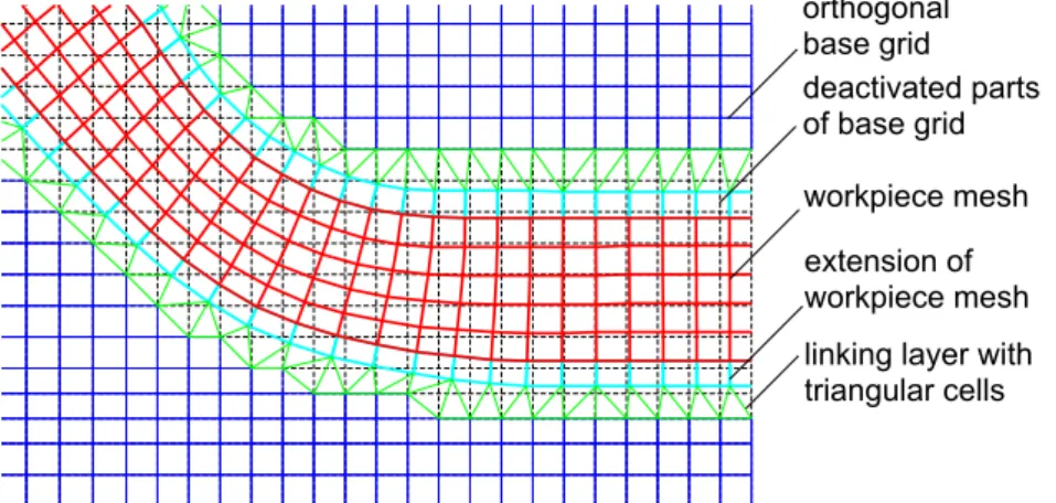
In contrast to [23], where the coupling of the moving structure to the orthogonal base grid is carried out by an interpolation strategy leaving the original base grid unaltered, here a remeshing procedure is applied. First, all grid cells of the base grid, which are totally or partially covered by the workpiece, as well as cells with nodes lying to close to the workpiece mesh are deactivated. Hence, an interior boundary in the base grid occurs. Then, the exterior workpiece contour and the resulting interior base grid contour are linked by triangular cells forming a co- herent mesh. Here, additional triangular cells occur, whenever nodes of the interior base grid contour are connected diagonally. In order to ensure that all nodes of the original workpiece mesh are adjacent to four quadrangular grid cells, an extended workpiece mesh with an addi- tional layer of nonconductive grid cells is used for the procedure described above. The topology regularized by this mesh extension is considered advantageous for the computation of nodal forces by evaluating Maxwell’s stress tensor. Figure 1 shows a detail of a mesh generated for a workpiece geometry at 63 µs, which resulted from the staggered EMAS-MARC coupling presented in [9]. As pointed out before, the coefficients for the generalized FD-scheme or Box-
w o r k p i e c e m e s h e x t e n s i o n o f w o r k p i e c e m e s h o r t h o g o n a l b a s e g r i d
l i n k i n g l a y e r w i t h t r i a n g u l a r c e l l s d e a c t i v a t e d p a r t s o f b a s e g r i d
Figure 1: Detail from remeshed Finite-Difference grid showing the workpiece mesh, its non- conductive extension and the linking layer to the remaining active base grid.
scheme can be derived in quite the same way as in the basic orthogonal grid by evaluating Ampere’s law. In order to obtain expressions for the magnetic field strength in a triangular cell depending on the nodal values ofΨ0, a linear approximation forΨ0 inzand r2in the triangle is chosen:
Ψ0(r, z) =c0+crr2+czz . (17) The constants c0, cr and cz are computable in dependence on the three nodal values Ψ0I, Ψ0II and Ψ0III by solving a linear system of equations. The coefficients cr andcz are related to the flux density components in the triangular cell as a result ofB~ = curlA:~
Bz = 2cr , Br(r) =−cz
r . (18)
The contribution to the circulation of the magnetic field around a node under consideration, which results from the part of the integrational path through the triangle from one edge to
another according to Fig. 2, can be calculated as follows:
Z MI,III
MI,II
H d~l~ = 1 µ
Z MI,III
MI,II
−cz
dr
r + 2crdz
. (19)
Since it does not depend on the path itself due to curlB~ = 0 for the field in (18) andµ=const.
rI , z I
r I I , z I I
rI I I , z I I I
Y I' Y I I' Y I I I'M I , I I
M I I , I I I
M I , I I I
Figure2: Triangular cell with nodes I, II and III, edge median pointsMI,II,MII,III andMI,III and part of integrational path (arrows) surrounding node under consideration, here No. I, along median lines.
inside the cell, simply a parametrized straight line can be assumed for evaluating (19). The constants cr and cz are replaced by the nodal values of Ψ0. Finally, a linear combination of these modified nodal vector potentials is obtained:
Z MI;III
MI,II
Hd~l~ =αI,IIΨ0II+αI,IIIΨ0III− αI,II+αI,III
Ψ0I. (20) Here, e.g. the coefficientαI,IIis given by
αI,II= 1 µ∆
(zIII−zI)(zIII−zII) +
rIII2 −rI2
lnrIII+rI rII+rI
(21) and∆stands for
∆=
rII2−rI2
(zIII−zI)−
r2III−r2I
(zII−zI). (22)
The logarithmic expression inαI,IIresults from integrating the 1/r-dependence. However, it can be shown that for large radii and comparably low radial distances of the nodes the coefficients αbecome approximately those expressions, which are obtained in rectangular coordinates (2D problems) for first order finite elements.
The quadrangular grid cells in the workpiece are treated in a similar way based on a subdivision of such a cell into four underlying triangles. The modified vector potentialΨ0cof the center point as the point in common for the four triangles is assumed to be a linear combination of the valuesΨ01...4of the quadrangle’s vertices with weighting coefficientsκ1...4depending on geometry and their sum equaling one. The paths of integration are led from the edge median points to the center point right through the adjacent triangle. The according contribution to the magnetic circulation under consideration depends on Ψ0c as well as on two vertex potentials.
After replacingΨ0c by the aforementioned linear combination only the vertex potentials occur and the resulting coefficients for matrix assembly are obtained.
In contrast to the base grid, where matrix assembly is carried out row by row, i.e. nodal
equation by nodal equation, for the nonorthogonal parts of the mesh the matrix is assembled by adding the contributions e.g. arsing from (21) to the coefficient matrix grid cell by grid cell, similar to matrix assembly in the Finite Element Method.
3.5 Timestepping
As time stepping for the electromagnetic subsystem the generalized trapezoidal rule has been chosen. Only the conductivity matrixB and the convective matrixChave to be reassembled in every time step, while the permeability matrix K does not change due to the choice of a fixed mesh. At the beginning of the process vibration due to the switching on of power have to be filtered out. Consequently the parameter of the generalized trapezoidal rule has to be chosen close to the backward Euler situation. Later, the optimal parameter yielding an acurracy of O(δt2) can be chosen, whereδtis the size of the time step.
In the FD-code the same method also known as θ-method is applied. According to the following approximation of integrals of a quantityq(t) over one time step
Z t+δt
t
q(τ)dτ= (1−θ)δtqt+δt+θδtqt, (23) θ = 0 results in the backward Euler formula, whereasθ= 0.5 is the mere trapezoidal rule. For the computations carried out here for θ a value of about a third has been chosen sometimes referred to as Galerkin approach. A moving mesh is used, so that the convective term does not occur explicitly. All contributions to electromagnetic induction, motion conditioned as well as arising from field variation, are included by evaluating the total derivative of the nodal modified vector potentialsΨ0. However, the reluctance matrix has to be regenerated in every time step.
3.6 Coupling Strategies
The coupling between the two subsystems is carried out in a staggered way. This means that the magnetic field distribution is calculated with respect to the position and velocity of the structure in thenth time step. After that the new position of the structure is determined such that a balance between inner and outer forces arises. However, benchmark simulation have shown that this algorithm can be improved by adding an additional iteration loop: To ensure that the computed momentum balance of the structure in the (n+ 1)st time step represents a balance between the Lorentz forces in the (n+ 1)st time step and the inner forces of the structure at this instant, the following scheme is applied: Let all values having index nbe variables of the nth time step. Then the update for the (n+ 1)st time step looks like this:
1. A predictor value A~(1n+1) for the vector potential and for its time derivative in the (n+ 1)st step is computed according to the measured amperage in the tool coil at time t(n+1)and the kinematic state of the workpiece. For this, the assembly routine of the magnetic mesh checks wether a certain point lies in the workpiece or not. The values for conductivity and for the velocity of the structure are chosen respectively.
2. The stiffness matrix and load vector in the workpiece mesh are assembled. For this, the nodal values of the current Lorentz force density are computed according to
fL(n+1)=J~1(n+1)×B~(n+1)1 =γ ∂tA~(n+1)1 ×curlA~(n+1)1 . (24)
3. The assembled equation in the workpiece mesh is solved. The computed deformations are added to the vertex positions of the workpiece mesh. It is checked, whether the residual force associated with the resulting state of deformation is zero in the scope of desired accuracy. If the latter is false, another step of the Newton-Raphson iteration has to be performed with the altered position of the workpiece. Otherwise, the vector potential A~(n+1)2 according to the new kinematic state of the structure is computed. If it does not deviate fromA~(n+1)1 within the scope of accuracy, the next time step is started. Otherwise, the equilibrium position of the structure with respect to outer forces resulting fromA~(n+1)2 and its time derivative is determined.
4. A series of vector potentials A~(n+1)k and corresponding equilibrium positions of the me- chanical structure is computed, untilA~(n+1)k+1 =A~(n+1)k within the scope of accuracy. Then a new time step is started.
Using the Finite-Difference code FELMEC for the electromagnetic subsystem one can set up an explicit coupling scheme, the accuracy of which is considered sufficient, if a small time step of e.g. 0.1 ... 0.2µs is chosen. Having calculated the nodal forces in the workpiece the electro- magnetic simulation has to be interrupted after each time step. The calculation of nodal forces is carried out by a local evaluation of Maxwell’s stress tensor on a surface around a node under consideration. The list of nodal forces is written out and passed to the structural mechanical part of SOFAR as a prescribed load, which calculates an update of the workpiece shape and mesh. With this updated mesh the electromagnetic computation is continued. Control and synchronization of the two processes are carried out by a shell script and JAVA-routines in SOFAR.
4 Validation by Benchmark Problems
Details of the implementation of the coupled electromagnetic field computation described above have been validated by several benchmark simulations involving comparisons with the pro- grams EMAS, FEMM and ANSYS. The mechanical side has been tested in [16]. Here we present a benchmark test that allows to validate the fully coupled simulation, where the above described FD-code serves as reference. Although many questions have already been clarified, the benchmark process and the optimization of SOFAR are still work in progress.
To validate whether SOFAR computes a correct force distribution, first a fully coupled simulation is carried out with SOFAR. Thereby the same geometry and input currency are re- garded as described in [16]. In particular, the mechanical side is simulated by an elastoplastic element. Although this modeling fails to account for the rate dependency of the mechanical structure it suffices for a validation of the electromagnetic field computation as it leads to ap- proximatively correct results (see [16] or [1, 2, 3, 9]). Next, the FD-code is coupled with SOFAR such that the computation of the electromagnetic field is carried out by the FD-Software, while SOFAR simulates the mechanical subsystem. The results of these simulations are compared to each other and to experimental results. Both simulations mirror the forming process qual- itatively correctly: Figure 3 shows the shape of the work piece after 35µs. The form of the work piece stays extremly similar during the whole forming process in both simulations. This
shows that both approaches, although completely different, are basically numerically equiva- lent for this example. Moreover, comparison to experimental data from [3, 4] shows that the
z
v o n M i s e s S t r e s s
8 0 1 0 1 1 2 2 1 4 3 1 6 4 1 8 6 2 0 7 2 2 8 2 4 9 2 7 0 2 9 1 M P a
S O F A R ( e l e c t r o m a g n e t i c a n d m e c h a n i c a l ) F E L M E C ( e l e c t r o m a g n e t i c ) a n d S O F A R ( m e c h a n i c a l )
r
Figure3: Workpiece contour and von Mises stress at instant of timet= 35µs
coupling of SOFAR with the FD-code leads to a satisfactory result*: Figure 4 shows the verti- cal displacement of the structure on the axis and at a radius of 21 mm for both simulations in comparison with experimental data. However, with the current parameters, SOFAR computes
0123456 0 5 1 0 1 5 2 0 2 5 3 0 3 5 4 0 5 0
t m s
z u p
m m
02468 1 0 1 2
0 5 1 0 1 5 2 0 2 5 3 0 3 5 4 0 5 0
t m s
z u p
m m S O F A R ( e l . & m e c h . )
F E L M E C ( e l . ) & S O F A R ( m e c h . ) M e a s u r e m e n t b y L f U
S O F A R ( e l . & m e c h . )
F E L M E C ( e l . ) & S O F A R ( m e c h . ) M e a s u r e m e n t b y L f U
Figure 4: Position of upper workpiece surface on axisr = 0 mm, graph on left hand side, and atr= 21 mm, graph on right hand side.
a slightly larger distribution of forces than the FD-simulation leading to more deformation of the work piece. In the beginning, both simulations yield nearly the same displacement but after 35 and 20 µs respectively the deviation becomes obvious achieving a value of about 2 mm after 60µs. This deviation is mainly caused by the different spatial discretizations used for electro- magnetic field computation (up to 47000 unknowns in the case of the FD-SOFAR simulation and 1126 unknowns for the SOFAR computation). The results of the simulation show that the discretization within SOFAR has been chosen much too coarse. To increase the accuracy of SOFAR without reducing its efficiency, adaptive meshing algorithms based on local error esti- mation will be implemented soon. Moreover, the choice of optimal numerical parameters is still work in progress and will be carried out with the help of further benchmark tests.
5 Conclusions
The algorithmic implementation of the electromagnetic subsystem of a fully coupled simulation tool for electromagnetic forming has been presented. Details of the realization of the underly- ing physical model are discussed. In particular, the tool coil is correctly modeled as massive
*Note that an elastoplastic model slightly overestimates the deformation of the workpiece (see e.g. [16]).
conductor with the help of an iterative scheme. Convective terms are accounted within the weak form of the field equations. The non linear coupling between the magnetical and me- chanical subsystem is performed in a staggered but implicit way, allowing for larger time steps.
The applied algorithms have been tested and optimized with the help of suitable benchmark tests. Although SOFAR can in principle cope with the computation of the Lorentz force distribu- tion coupling the electromagnetic system and the mechanical structure, further improvements concerning the accuracy of the field computation are necessary to obtain full accordance to experimental data. In particular, numerical algorithms for error control and adaptive refinement have to be implemented and validated by further benchmark simulations. This will improve SOFAR to a convenient and reliable tool for the simulation of EF forming processes.
References
[1] C. Beerwald, A. Brosius, W. Homberg, M. Kleiner, and A. Wellendorf. New aspects of electromagnetic forming. InProceedings of the 6th International Conference on the Tech- nology of Plasticity, volume III, pages 2471–2476, 1999.
[2] C. Beerwald, A. Brosius, and M. Kleiner. Determination of flow stress at very high strain- rates by a combination of magnetic forming and fem calculation. In Proceedings of the International Workshop on Friction and Flow Stress in Cutting and Forming (CIRP). EN- SAM - Paris, 2000.
[3] M Badelt, C. Beerwald, A Brosius, and M. Kleiner. Process analysis of electromagnetic sheet metal forming by online-measurement and finite element simulation. InProceedings of the 6th International ESAFORM Conference on Material Forming, 28.-30. April 2003, Italy, pages 123–126. ESAFORM 2003, 2003.
[4] C. Beerwald, A. Brosius, M. Kleiner, and V. Psyk. Einfluss des magnetischen Druckes bei der elektromagnetischen Blechumformung. In2. Kolloquium Elektromagnetische Um- formung. Forschergruppe “Untersuchung der Wirkmechanismen der elektromagnetischen Blechumformung”, 2003.
[5] W. H. Gourdin. Analysis and assessment of electromagnetic ring expansion as a high- strain rate test. J. Appl. Phys., 65:411, 1989.
[6] W. H. Gourdin, S. L. Weinland, and R. M. Boling. Development of the electromagnetically- launched expanding ring as a high strain-rate test. Rev. Sci. Instrum., 60:427, 1989.
[7] N. Takata, M. Kato, K. Sato, and T. Tobe. High-speed forming of metal sheets by electro- magnetic forces. Japan Soc. Mech. Eng. Int. J., 31:142, 1988.
[8] G. Fenton and G. S. Daehn. Modeling of electromagnetically formed sheet metal. J.
Mat. Process. Tech., 75:6–16, 1998.
[9] C. Beerwald, A. Brosius, W. Homberg, M. Kleiner, M. Klocke, and S. Kulig. Extended finite element modelling of electromagnetic forming. In Proceedings of the 10th International Conference, 14.-16. April 2003, United Kingdom, pages 559–566. SheetMetal 2003, 2003.
[10] B. Svendsen and T. Chanda. Continuum thermodynamic modeling and simulation of electromagnetic forming. Technische Mechanik, 23:103–112, 2003.
[11] B. Svendsen and T. Chanda. Continuum thermodynamic formulation of models for elec- tromagnetic thermoinlastic materials with application to electromagnetic metal forming.
Cont. Mech. Thermodyn., 2004. submitted.
[12] A. Brosius, M. Kleiner, and B. Svendsen. Finite-element modeling and simulation of the material behaviour and structural behaviour during electromagnetic metal forming of metal tubes and sheet metal. 2003. in preparation.
[13] A. Brosius, T. Chanda, M. Kleiner, and T. Svendsen. Finite-element modeling and simula- tion of material behavior during electromagnetic metal forming. InProceedings of the 6th International ESAFORM Conference on Material Forming 28.-30. April 2003, Italy, pages 971–974. ESAFORM 2003, 2003.
[14] M. Stiemer, J. Unger, H. Blum, and B. Svendsen. Algorithmic formulation and numerical implementation of coupled multifield models for electromagnetic metal forming simulations.
2004. in preparation.
[15] H. Blum, H. Kleemann, A. Rademacher, T. Rauscher, A. Schroeder, and M. Stiemer. SO- FAR. www.mathematik.uni-dortmund.de/lsx/sofar, 2003.
[16] M. Kleiner, A. Brosius, H. Blum, F. T. Suttmeier, M. Stiemer, B. Svendsen, J. Unger, and S. Reese. Benchmark problems for coupled electromagnetic-mechanical metal forming processes. Annalen der wissenschaftlichen Gesellschaft f¨ur Produktionstechnik, 2004. in press.
[17] F. Moon. Magnetic interactions in solids. Springer-Verlag, 1980.
[18] M. Schinnerl, J. Sch ¨oberl, M. Kaltenbacher, and R. Lerch. Multigrid methods for the 3d simulation of nonlinear magneto-mechanical systems. IEEE transactions magnetics, 38:1497–1511, 2002.
[19] J. C. N´ed´elec. Mixed finite elements inR3. Numerische Mathematik, 35:315–341, 1980.
[20] J. C. N´ed´elec. A new family of mixed finite elements in R3. Numerische Mathematik, 50:57–81, 1986.
[21] Ch. Großmann and H.-G. Roos. Numerik partieller Differentialgleichungen. Teubner Stu- dienb¨ucher-Mathematik, Stuttgart, 1994.
[22] S. Kulig, M. Klocke, A. Joswig, D. Peier, and M. Hinck. Modellierung und Simulation der nichtlinearen elektromagnetischen kopplung zwischen Werkst¨uck und Umformspule. In Kolloquium elektromagnetische Umformung 2003, 2003.
[23] M. Klocke. Computation of axisymmetric transient electromagnetic fields by finite- difference schemes including prescribed motion. In6. International Symposium on Electric and Magnetic Fields (EMF) 2003, 2003.