Essays On the Optimal Interplay of Early and Late Education Subsidies and Taxation

and L ate E ducation S ubsidies and T axation

Inauguraldissertation zur Erlangung des Doktorgrades der Wirtschafts- und Sozialwissenschaftlichen Fakultät der Universität zu Köln

2019

vorgelegt von

Dipl.-Volksw. Fabian Becker

aus Düsseldorf

Korreferent: Prof. Dr. Martin Barbie

Tag der Promotion: 17.07.2019

Zuallererst möchte ich mich bei meinem Betreuer, Alexander Ludwig, bedanken. Durch seine leidenschaftliche Art zu unterrichten und die engagierte Betreuung im Rahmen meiner Diplo- marbeit, ist er für mich einer der Hauptgründe gewesen, das Promotionsstudium zu beginnen.

Zudem konnte ich mich über den gesamten Verlauf meiner Dissertation voll auf seine Unter- stützung verlassen und habe sehr viel davon profitieren können. Mein Dank gilt auch Dirk Kruger, der mir neben der sehr wertvollen Zusammenarbeit ein Semester an seinem Lehrstuhl an der University of Pennsylvania ermöglicht hat. In dieser Zeit konnte ich viel aus dem inspiri- erenden Arbeitsumfeld, seinem Unterricht und den Diskussionen mit tollen Kollegen lernen.

Des Weiteren möchte ich mich bei Martin Barbie bedanken, der mir zusammen mit Alexander Ludwig den Spagat aus einer Dissertation in Köln und Frankfurt ermöglicht hat.

Ich habe sowohl in Köln als auch in Frankfurt großes Glück mit meinen Kollegen gehabt.

Ganz besonders möchte ich mich bei Raphael Flore und Alexander Stolz bedanken, die in der gemeinsamen Zeit an der CGS zu Freunden geworden sind. Aus der Zeit in Frankfurt fällt es mir schwer, einzelne Personen herauszunehmen, da die Stimmung grundsätzlich eine extrem gelöste und kollegiale war. Das tri ff t insbesondere auf die gemeinsamen, wettkampfgeprägten Workshops und Team-Ausflüge zu, bei denen uns Alex stets hat “gewinnen lassen”. Trotz- dem möchte ich mich im Einzelnen bei Raphael Abiry, Nils Grevenbrock und Jorge Quintana für wertvolle Tipps zum Umgang mit Hochleistungsrechnern, bei Zhao Jin, Irina Popova und Osman Kucuksen für den fachlichen Austausch zu unserer Arbeit, und bei Christine Nieraad für all die Hilfe beim organisatorischen Drumherum, bedanken. Zudem bin ich auch Daniel Harenberg sehr dankbar, der mir den Start in die Welt des Programmierens stark erleichtert hat.

Persönlich möchte ich mich zuallererst bei meinem Vater bedanken - meinem größten Un-

terstützer. Roy bin ich neben seinem mentalen Beistand für seine o ff enen Ohren bei meinen

Monologen zu High Performance Computing dankbar, die nur mit der Empathie eine Freundes

zu ertragen gewesen sein können. Zum Schluss möchte ich mich bei Iga bedanken, meiner

besten Freundin, die jeden Tag zu einem Besseren macht und der ich diese Dissertation widme.

Contents

1 Introduction 1

2 A Model for the Interplay of Early and Late Education Subsidies and Taxation 10

2.1 Environment . . . . 10

2.2 Human Capital and College Education . . . . 13

2.2.1 Human Capital Process . . . . 14

2.2.2 Labor Productivity and Wages . . . . 15

2.2.3 Dynamic Complementarity and Self-Productivity . . . . 16

2.3 Market Structure . . . . 20

2.4 Government Policies . . . . 21

2.5 Time Line . . . . 22

3 Solving the Household Problem 26 3.1 Recursive Problem of Households . . . . 26

3.2 Hybrid Solution Methods . . . . 32

3.2.1 Analytical Solution of a Two-Period Model . . . . 33

3.2.2 Endogenous vs. Exogenous Hybrid Method . . . . 36

3.3 Taste Shocks at College Decision . . . . 44

3.4 Policy Functions Education . . . . 47

3.5 A Glance at the Numerical Computation . . . . 51

4 Calibration 53 4.1 Demographics . . . . 53

4.2 Preferences . . . . 53

4.3 Human Capital Grid and Intergenerational Transmission . . . . 54

4.4 The Human Capital Process . . . . 54

4.5 Labor Productivity Process . . . . 56

4.6 Education Costs and Subsidies . . . . 59

4.7 Borrowing Constraints . . . . 60

4.8 Government . . . . 61

4.9 Prices . . . . 62

4.10 Calibration of Second Stage Parameters . . . . 63

4.11 Lifecycle Plots of Benchmark Model . . . . 64

5 Partial Equilibrium Analysis 68 5.1 College Subsidies . . . . 69

5.2 Non-Tertiary Investments . . . . 75

5.3 Tertiary and Non-Tertiary Education Measures . . . . 79

5.4 Summary Partial Equilibrium Experiments . . . . 82

6 Small Open Economy 85 6.1 College Subsidies . . . . 86

6.2 Non-Tertiary Investments . . . . 88

6.3 Tertiary and Non-Tertiary Education Measures . . . . 89

6.4 An Outlook on General Equilibrium . . . . 91

7 Conclusion 93 A Appendix to Chapter 2 103 A.1 Our Model in Light of the Human Capital Literature . . . 103

A.1.1 Adjacent Research . . . 105

B Appendix to Chapter 3 108 B.1 Reformulation of the Household Problem . . . 108

B.1.1 Cash-On-Hand Definition and Asset Regions . . . 108

B.1.2 Savings Under New Cash-On-Hand Definition . . . 110

B.1.3 Recursive Problem of Households in Terms of Cash-On-Hand . . . 113

B.2 Solving via Endogenous Grid Method . . . 122

B.2.1 Smart Savings Grid Construction . . . 125

B.3 Solving via Hybrid Exogenous Grid Method . . . 128

B.3.1 Solving via Exogenous Grid Method . . . 128

B.3.2 Solving for Inter-Vivos Transfers . . . 131

B.3.3 Solving for Human Capital Investments . . . 133

B.4 An Incorrect Hybrid Solution Method . . . 136

B.4.1 Solving for Inter-Vivos Transfers . . . 137

B.4.2 Solving for Human Capital Investments . . . 139

B.5 Solving for Consumption and Leisure . . . 141

B.5.1 Interior Solution of Consumption and Leisure . . . 143

B.5.2 Binding Leisure Constraint . . . 145

B.5.3 Binding Borrowing Constraint . . . 145

B.6 Taste Shocks . . . 149

B.7 Budget in College . . . 152

B.8 Parallelization . . . 154

C Appendix to Chapter 4 156 C.1 Households . . . 156

C.2 Ability and Education . . . 157

C.3 Labor Productivity and Wages . . . 158

C.4 Government and Pension Budget . . . 159

C.5 GE Interpretation of PE Model . . . 162

C.6 Calibration in Partial Equilibrium . . . 164

C.7 Prices in General Equilibrium and Small Open Economy . . . 166

C.8 Aggregation . . . 167

C.9 Transformation in 4-Year Model . . . 170

D Appendix to Chapter 5 172 D.1 Inequality Measures . . . 172

E Appendix to Chapter 6 176

List of Figures

1 Time Line . . . . 25

2 Decisions as a Function of Cash-On-Hand (COH) . . . . 37

3 Savings and Investments Under Di ff erent Solution Methods . . . . 42

4 HybLevEndo in Special Scenarios . . . . 43

5 Situation at College Without Taste Shocks . . . . 44

6 Situation at College With Taste Shocks . . . . 46

7 Parental Investments in Primary and Secondary Edu. . . . 48

8 Secondary Investments Given Abilities . . . . 49

9 Vivos Transfers and the College Decision . . . . 50

10 Ability Gaps Open Up Early . . . . 66

11 Life-Cycle Profiles . . . . 67

12 Experiment College Subsidy ( *Benchmark Model) . . . . 70

13 Comparison Human Capital Development . . . . 73

14 Experiment Non-Tertiary Investments ( *Benchmark Model) . . . . 76

15 Human Capital Development Given ¯ i

/w

= 0.0978 . . . . 77

16 Experiment Tertiary and Non-Tertiary Education . . . . 79

17 Human Capital and College . . . . 81

18 Labor Tax Rate . . . . 82

19 Results Univariate Experiments (SOE) . . . . 86

20 Human Capital Development (θ = 175%) . . . . 88

21 Results Bivariate Experiment (SOE) . . . . 90

22 Comparison Results Non-Tertiary Investments . . . . 91

23 Labor as a function of cash-on-hand . . . 111

24 College Attendance Probability . . . 151

25 Results Bivariate Experiment (SOE) . . . 181

26 Experiment College Subsidy General Equilibrium ( *Benchmark Model) . . . 182

List of Tables

1 Educational CVs . . . . 16

2 HybLevEndo and ¯ A = 10 (B = 0, ¯ i = 2, ν = 0.5) . . . . 39

3 HybLevEndo and ¯ A = 14 (B = 0, ¯ i = 2, ν = 0.5) . . . . 40

4 Comparison Computational Time . . . . 52

5 Calibration . . . . 57

6 Estimates for Earnings Process and Markov Chain for Wages . . . . 58

7 Summary Economic Second Stage Parameters . . . . 63

8 Results Policy Experiments Partial Equilibrium . . . . 69

9 Results Production . . . . 71

10 Results Education . . . . 72

11 Results Equality . . . . 74

12 Results Production . . . . 75

13 Results Education . . . . 77

14 Results Equality . . . . 78

15 Comparison Univariate and Bivariate Optima . . . . 83

16 Results College Subsidy Experiment (SOE) . . . . 87

17 Results Non-Tertiary Investments Experiment (SOE) . . . . 89

18 Comparison Computational Time “ToyModel_Parallel” . . . 154

19 Transformation Production in 4-Period Model . . . 171

20 Full Results Partial Equilibrium Experiment Subsidies . . . 173

21 Full Results Partial Equilibrium Experiment Non-Tertiary Investments . . . 174

22 Full Results Small Open Economy Experiment Subsidies . . . 177

23 Full Results Small Open Economy Experiment Non-Tertiary Investments . . . 178

24 Full Results General Equilibrium Experiment Subsidies . . . 179

25 Full Results General Equilibrium Experiment Non-Tertiary Investments . . . . 180

1 Introduction

A benevolent government that aims to increase welfare can employ various means in order to eliminate or mitigate market failures. An important example is the use of progressive taxa- tion in order to reduce negative consequences of uninsurable, idiosyncratic income risk. Such interventions in the market, however, may lead to other ine ffi ciences, since they distort house- hold decisions. Progressive taxation, for instance, distorts the labor supply. And in addition, it distorts the incentive to reach for higher education, as it implies a relative decrease of the net income for higher skilled jobs. Addressing this trade-o ff , Krueger and Ludwig (2013) and Krueger and Ludwig (2016) develop a quantitative model that shows that college subsidies are a valuable tool to counteract the distorting e ff ect of progressive taxation on educational decisions.

Thus their papers are to be seen in the intersection of two strands of literature - on the one hand the literature on optimal income taxation and on the other hand a previously rather theoretical literature, dealing with the optimal combination of progressive income taxes and educational subsidies in models that abstract from idiosyncratic risk.

The extension of the work of Krueger and Ludwig, which is made in this thesis, links it additionally to the literature on human capital production of young people.

This literature em- phasizes the di ff erences in the formability of skills in the various stages of ability development across the life-cycle, and draws attention especially to the early years. Due to the dynamic- complementary nature of the human capital process, it is hardly possible to compensate for missed early investments in education at later stages. Hence, when this foundation is not built when children are young, for example, a subsequent college education will hardly be possi- ble, regardless of its costs.

The key contribution of this thesis is thus to expand the model of Krueger and Ludwig by analyzing the endogenous formation of the human capital that people

1

See Cunha and Heckman (2010) for a comprehensive summary of the literature on the production of skills of young people.

2

Cunha, Heckman and Schennach (2010) dissect the skill formation process of children and estimate a multi-

stage human capital production function, taking into account the empirical facts of the literature summarized in

Cunha and Heckman (2010).

already have when they start into their adult life. This analysis takes into account parents’ invest- ments in primary and secondary education in response to college subsidies. These investments, in turn, have a major impact on the e ff ectiveness of the subsidies. Additionally, the college pro- cess is further refined in this thesis. Students achieve a degree with a success probability that is dependent on their human capital. Hence, with college dropouts a third qualification status is introduced and the tertiary education process is modeled more realistically.

While early investments in human capital are very important, they di ff er across socioeco- nomic groups. In this context, the literature on human capital shows a high level of persistence of income over generations, which in addition to the inheritance of skills comes in particular from better access to education for children of better-earning households.

In this thesis, the government will have the opportunity to choose over not only college subsidies but also its in- vestments in primary and secondary education. Although intergenerational immobility is not the focus of this thesis per se, it points to another market failure, when human capital can not flourish because of low innate abilities, but because of the lack of financial resources of parents.

As a result, I will show that the e ff ectiveness of college subsidies and non-tertiary investments are dependent on each other, and by incorporating both instruments, the government can opti- mally balance the interplay of early and late education subsidies.

This thesis is structured as follows. In Chapter 2, I develop a model that, building on the work of Krueger and Ludwig, involves the human capital process during primary and secondary education. In doing so, I will analyze which mechanisms from the human capital literature are relevant to the problem at hand and where they find themselves in the model. In particular,

3

Solon (2002) provides a cross-country survey of intergenerational mobility. Restuccia and Urrutia (2004) dis- sect the source of intergenerational persistence and stress the importance of early education investments. Blanke- nau and Youderian (2015) discuss how intergenerational persistence in earnings can be explained by government spending in early education.

4

In a quantitative analysis Caucutt and Lochner (2017) show that ignoring the earlier investment responses may lead to a significant under-estimation of the impact of college subsidies and emphasize the importance of borrowing constraints of families at early stages. Findeisen and Sachs (2016) show that governmental education loans to young households combined with income-contingent repayment can be designed in a Pareto optimal way.

In recent work, Lee and Seshadri (2019) underline the importance of financial frictions in early years for the

persistence of economic status.

self-productivity and dynamic complementarity are key elements and I will show that these concepts are incorporated in all stages of human capital development in this thesis, i.e. primary, secondary and tertiary education.

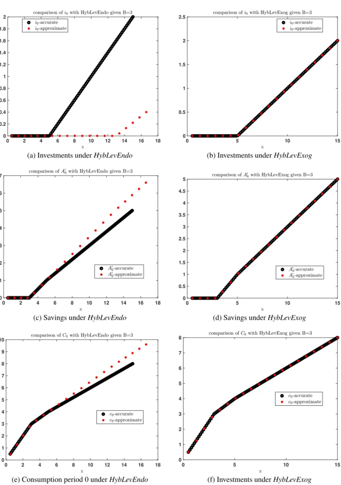
Chapter 3 deals with the solution algorithm of the model. First, I show that the combination of endogenous grid method and level search over the value function used in Krueger and Ludwig (2013) leads to inaccuracies. In this thesis, an alternative solution method is developed, which delivers accurate results. This is illustrated using a two-period model, which is first solved analytically and then quantitatively under both solution methods. By comparing household decisions based on di ff erent cash-on-hand levels, the solution method in Krueger and Ludwig (2013) does not address the trade-o ff between consumption, savings and investments correctly and thereby underestimates the investment choice. In addition, the region in which households are borrowing constraint is not identified precisely, when situations occur in which savings are zero but human capital investments are positive.

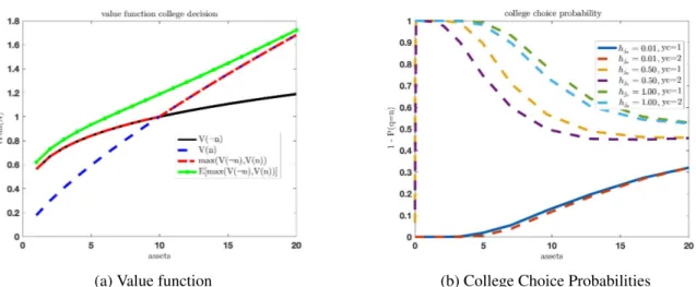
In a second step, I extend the model of Krueger and Ludwig (2013) by introducing taste shocks to avoid kinks in the value function and jumps in first order conditions that would otherwise be caused by the discrete college decision.

Next, I build a bridge to Chapter 2 by showing that the model’s policy functions are consistent with the mechanisms of the human capital literature. I conclude this part with a quick look at the quantitative computation, in particular the parallelization of the solution algorithm, which was necessary for this complex model to be solved in a timely manner.

In Chapter 4, the model is calibrated to the core moments of the underlying problem. In addition to education-specific targets such as college attendance and college wage premium, this will be about a realistic representation of the government’s budget and its expenditures in tertiary and non-tertiary education. Similar to the previous part, I conclude this chapter by showing that the life-cycle profiles resulting from the calibrated benchmark model are consistent with the findings from the human capital literature.

In Chapter 5, three policy experiments are conducted in partial equilibrium, in which wages

5

This applies for both the solution of optimal vivos transfers and investments in primary and secondary educa-

tion. While only the former are included in the paper of Krueger and Ludwig, in this thesis, this issue would spill

over to the human capital investment periods of parents as well.

do not react to shifts in the labor market. Initially, the government can optimize either college subsidies or investments in non-tertiary education, while the other policy instrument remains at the level of the benchmark model. In both experiments, the welfare optimum is above the current status quo. However, these two univariate experiments show, that the two policy in- struments work through di ff erent channels. College subsidies lead to a higher aggregate human capital as parents respond with an endogenous increase in their primary and secondary educa- tion investments. But this does not lead to a more equal distribution of income and consumption, since the human capital of children from education and income-poor households increases the least by this policy measure. By contrast, higher governmental investments in non-tertiary ed- ucation lead to an increase in human capital across all income and education groups and, in addition to an increase in aggregate production and consumption, to a more equal distribution.

Still in partial equilibrium, I then conduct a bivariate experiment, in which the government can determine both investments in non-tertiary education and college subsidies. It becomes appar- ent, that the e ff ectiveness of college subsidies depends on the level of non-tertiary education investments - and vice versa. In a nutshell, this is because the benefits of college subsidies can only be claimed if the young adults have the skills to successfully complete college. Early investments lead to a high human capital level, but this potential remains unused and is not translated into higher wages, if college education can only be a ff orded by a small fraction of households. If investments are kept to a minimum, for example, one could come to the mislead- ing conclusion that college subsidies are not an e ff ective tool in increasing college attendance and welfare. In the bivariate optimum of partial equilibrium, both policy instruments are above their respective values of the benchmark model. Consequently, aggregate levels of production and consumption are higher while their distributions are more equal than in the status quo.

In Chapter 6, I will perform the same experiments in a small open economy setup, in which wages do react to changes in the labor market, but the interest rate remains constant.

This

6

This intermediate step allows to disentangle the e ff ects from the labor market and the capital market. In

addition, computationally, the small open economy experiments converge much faster than the general equilibrium

experiments. This was crucial in order to perform bivariate experiments due to restrictions of high performance

computing resources.

will allow the college wage premium to adapt to shifts in the labor market. As a result, the di ff erences with respect to the impact of the two policy instruments on the distribution of the economy are less sharp than in partial equilibrium, but they continue to work thorough di ff erent channels. Subsidies accomplish equality by a reduction in the college wage premium, while investments in non-tertiary education not only shift aggregate human capital to a higher level, they also accomplish a denser distribution of skills. The other results, however, are transferred from the partial equilibrium to the small open economy: (i) the e ff ectiveness of one policy instrument depends on the level of the other, (ii) therefore univariate experiments can lead to misleading results and (iii) the optimal interplay of the two policy instruments is accomplished at a higher level for both college subsidies and non-tertiary education investments compared to their respective values from the benchmark model, financed by a higher labor tax rate.

In Chapter 7, I will summarize the results and give an outlook on other aspects that should be considered in future work related to this thesis.

Brief Summary of the Model Structure

The model allows the government to set up a progressive tax scheme and to use revenues to

grant college subsidies as well as to invest in early human capital. In order to analyze the

respective interactions, a life-cycle model with endogenous educational choices, labor supply

and consumption-savings decisions in presence of risky labor productivity and borrowing con-

straints is developed. Educational investments of parents into their children take place at all

stages of the child’s life-cycle. When children reach adulthood, they decide whether or not to

attend college, which relies on four key aspects. First, college education is costly, both in terms

of time and monetary resources. Second, parents can transfer resources to their children which

may relax potential financial constraints. Third, average wages of college graduates exceed

those of non-college workers. Fourth, the success probability in college and the distribution of

wages around mean wages over the life-cycle depends on the acquired human capital at the time

of the college decision.

A benevolent government may a ff ect all these margins through the choice of the three poli- cies measures mentioned above: early education subsidies (primary and secondary), college subsidies (tertiary education) and progressive income taxes. The latter provide insurance against idiosyncratic labor productivity risk and redistribute across di ff erent types of workers, who can di ff er in education and their respective productivity. However, by intervening in the tax system, the government distorts labor supply and, given that the return on investments in human capital is expressed in higher net wages, the distortion also a ff ects educational decisions. The govern- ment may mitigate the latter through education subsidies. But then the question arises, how to optimally design an educational system. Are education subsidies su ffi cient to improve the distribution of resources? How exactly do early and late education subsidies and progressive income taxes interact?

In order to address these questions, the life-cycle model is further embedded into a macroe- conomic framework through which general equilibrium repercussions are acknowledged, that play an important role. For instance, increasing subsidies to tertiary education will increase the number of college workers relative to non-college workers. In a small open economy or general equilibrium, this increased abundance of college workers reduces the college wage premium which has welfare enhancing redistributional implications.

Related Literature

This thesis finds itself in the intersection of di ff erent strands of the literature and can be seen as an extension of the work of Krueger and Ludwig (2013) and Krueger and Ludwig (2016).

Krueger and Ludwig (2013) characterize the optimal policy mix of capital income taxes, pro-

gressive labor income taxes and education subsidies in a model with income risk, borrowing

constraints and endogenous human capital formation. They conclude that both the degree of tax

progressivity as well as education subsidies for college education should be higher than in the

current U.S. status quo. Krueger and Ludwig (2016) extend this earlier work by accounting for

the feedback from an increase of the share of workers with a college degree on the college wage

premium. Through this general equilibrium feedback education subsidies are a powerful instru- ment to achieve redistributional objectives. To mitigate distortions, tax progressivity should be reduced, especially along the economy’s transition to a new steady state. The optimal policy is therefore characterized by higher education subsidies and lower progressivity than under the current status quo.

Their work is located in the intersection of two bodies of literature. First of all the litera- ture on optimal income taxation, which examines the optimal income tax code a Ramsey type government

should implement in a quantitative OLG model,

when uninsurable idiosyncratic income risk is present

. In addition, their work is connected to a previously rather theoretical literature, studying the optimal combination of progressive income taxes and educational sub- sidies in models that abstract from idiosyncratic risk. By building up on the work of Krueger and Ludwig this thesis also incorporates both these strands of literature and the references they make.

By adding to the model the entire human capital process of primary and secondary educa- tion, this work additionally opens up to the literature on the production of skills of young people.

Cunha and Heckmann (2010) provide a detailed overview of empirically established facts and the mechanisms models need to incorporate in order to be able to acknowledge them.

They emphasize the self-productive and dynamic complementary nature of skill production, implying that higher investments at early stages increase the return on investments in all following stages of human capital formation. Against the background of these results, Cunha, Heckman, and Schennach (2010) estimate a multistage human capital production function capable of taking all of these facts into account.

These properties of human capital development pave the way for intergenerational persis- tence of earnings.

One measure for this persistence frequently used in the literature is the

7

See Chamley (1986) and Judd (1985).

8

See Auerbach and Kotlikoff (1987).

9

See Bewley (1986), Huggett (1993, 1997) and Aiyagari (1994).

10

These these facts and findings will be discussed in more detail below, when I describe how the educational process is designed in this thesis.

11

Solon (1999) starts with a very memorable illustration to highlight the importance of intergenerational per-

sistence when considering equality in a society. In a cross-sectional analysis two countries with the same Gini

slope coe ffi cient received by regressing log earnings of children (when they become adults) on log earnings of parents. A general finding is a high intergenerational persistence of earnings in the US. Following Stokey (1998) and Solon (1999) roughly 40% of the relative earnings posi- tion is passed from parents to their children.

At first glance, the intergenerational persistence is more of a philosophical aspect to this thesis and the underlying research question, since my welfare evaluation does not take intergenerational persistence into account. However, on closer inspection it points to a second ine ffi ciency - despite the distorting e ff ects of a progressive tax code - the government may address. In order to identify the reasons for intergenerational per- sistence and cross-sectional inequality of earnings, Restuccia and Urrutia (2004) set up a model where they allow three di ff erent sources to be their main drivers: innate ability, early education and college education. In a quantitative analysis they find that the half of the 40% of intergen- erational persistence is accounted for by di ff erences in early education.

Looking at these results together, the question arises as to what the di ff erences between the primary and secondary education of children are due to. Kaushal, Magnuson and Waldfogel (2011) arrive at the conclusion that parents in the top 20% spend 9% of their income on educa- tional enrichment items whereas parents in the bottom income quintile only spend 3% of their income. In a similar context Caucutt and Lochner (2017) investigate the importance of bor- rowing constraints of families at early stages. They find that a $10, 000 increase in discounted annual income of parents when children are at the age of zero to eleven reduces high school drop out rates by 2.5 percentage points, while it increases college attendance by 4.6 percentage points. Regarding the same increase at age 12 to 23 the e ff ect is not only much smaller but also

coe ffi cient would be considered as equal unequal. But adding the intergenerational information that in one of these countries children end up at the exact same position in the income distribution as their parents with certainty, whereas in the other country this is completely random, the second society would be considered as providing more equal opportunities.

12

Canada’ slope coefficient is by about 23% and Finland’s is about 22% (Solon 2002). Wiegand (1997) performs a similar regression for Germany and arrives at a persistence of 34%.

13

The other half is explained by intergenerational persistence of innate ability, whereas college education drives the extent of cross-sectional disparity, but does not explain its origin.

14

In a more recent study Blankenau and Youderian (2015) discuss how intergenerational persistence in earnings

can be reduced by government spending in early education, where they use the estimates of Cunha, Heckman and

Schennach (2010) to set up their human capital production function.

statistically insignificant.

Caucutt and Lochner refine this result, highlighting the importance of endogenizing the human capital process to analyze the impact of college subsidies. In a quantitative analysis they show that ignoring the earlier investment responses may lead to a significant under-estimation of the total wage impact of college-age investment subsidies by around 60%.

In summary, the literature on optimal income taxation shows that the government can imple- ment a progressive tax code to compensate ine ffi ciencies caused by uninsurable idiosyncratic income risk. Krueger and Ludwig have shown that college subsidies are a valuable tool to coun- teract the distorting e ff ects of progressive tax codes on labor and education related decisions.

However, the literature on human capital suggests that a change in college subsidies will lead to endogenous adjustments that in turn a ff ect their e ff ectiveness. In addition, evidence from this literature suggests that policies aimed at early education are the more powerful tool in shaping skills and thereby counter intergenerational persistence, which is not due to the inheritance of skills, but to access to education in childhood.

The contribution of this thesis to this literature is a large-scale OLG model that takes into ac- count all core mechanisms of the human capital literature and allows for endogenous responses within the whole human capital process of primary, secondary and tertiary education to changes in college subsidies and non-tertiary education investments by the government. By embedding this in a large-scale OLG environment, I am able to compare and quantify the di ff erent paths of impact of the two policy instruments in a realistic framework. By contrasting the results of the univariate with the bivariate policy experiments in both partial equilibrium and a small open economy setup, the di ff erences of the two policy measures could be highlighted very clearly. I quantify how the interplay of the policy instruments a ff ects distributional aspects of the econ- omy, human capital formation, and ultimately welfare. In addition, inaccuracies of the solution method used in Krueger and Ludwig (2013) were identified and corrected.

15

Among others, in earlier work Bohacek and Kapicka (2008) and Bohacek and Kapicka (2012) allow for

endogenous human capital accumulation in models with education subsidies.

2 A Model for the Interplay of Early and Late Education Subsidies and Taxation

Everything that follows is based on collaborative work of Dirk Krueger, Alexander Ludwig and myself.

Large parts of the model we now develop are based on the work of Krueger and Ludwig (2013) and Krueger and Ludwig (2016). The key di ff erence is, that they consider human capital at the age of the college decision to be exogenous. In our model, the formation of human capital is a core element and is shaped by the investments of government and parents during primary and secondary education. In addition, by introducing a stochastic college outcome, which is dependent on the human capital of the student, we refine the tertiary education process.

Therefore, this chapter is organized as follows:

We start with a rather brief description of the parts of the model that are borrowed from Krueger and Ludwig. We will then describe the extensions we make in great detail in Section 2.2. In particular, it will be about demonstrating how our model approach does justice to the literature on human capital production.

2.1 Environment

Demographics Population grows at the exogenous rate χ. We assume that parents give birth to children at the age of j

and denote the fertility rate of households by f , both assumed to be

16

We thank the participants of CMR Lunch Seminar and the Money and Macro Brown Bag Seminar at Goethe University Frankfurt for great feedback in the early phase of this project. All stages of the project were supported by great comments of the participants of the Reading Group on Quantitative Macroeconomics at Goethe University Frankfurt. We also thank the participants of the CEPR Workshop Financing Human Capital and the participants of the conference Human Capital and Financial Frictions at the Georgetown University.

17

I gratefully acknowledge financial support of the Land North Rhine Westphalia.

the same across education groups.

Notice that f is also the number of children per household.

Further, agents live with certainty until age J. The population dynamics are then given by N

= f · N

, N

= N

, ∀ j = 0, . . . , J − 1. (1)

Observe that the population growth rate is given by χ = f

1

1+j f

− 1. (2)

Furthermore, we denote by j

< j

the age of adulthood (i.e., the age when children leave the household, form an own adult household and make the college attendance decision) and by j

> j

the retirement age ( j

− 1 is the last working age before retirement).

Technology We distinguish between workers according to their qualification q ∈ { n, c, d } , where q = n denotes non-college workers (without any attendance at college), q = c denotes workers who completed college and q = d workers who attended but dropped out of college.

We assume that non-college workers and dropouts are perfect substitutes in production, whereas these two types of labor are imperfectly substitutable in production with respect to college work- ers (see Katz and Murphy (1992) and Borjas (2003)). Within each qualification-group labor is perfectly substitutable across di ff erent ages. Let L

denote aggregate labor of qualification group q, measured in e ffi ciency units and let K

denote the capital stock. Total labor e ffi ciency units at time t, aggregated across the three qualification groups, is then given by

L

=

(L

+ L

)

+ L

=

L

+ L

, (3)

18

Note that due to the endogeneity of the education decision in the model, if we were to allow di ff erences in the

age at which households with di ff erent education groups have children it would be hard to assume that the model

has a stationary joint distribution over age and skills.

where L

≡ L

+ L

. Aggregate production follows a nested CES-Cobb-Douglas production function, reading as

Y

= F(K

, L

) = K

(L

)

= K

L

+ L

. (4)

Perfect competition among firms and constant returns to scale in the production function imply zero profits for all firms and an indeterminate size distribution of firms. Thus, there is no need to specify the ownership structure of firms in the household sector, and without loss of generality we can assume the existence of a single representative firm.

This representative firm rents capital and hires the two skill types of labor on competitive spot markets at prices r

+ δ and w

, where r

is the interest rate, δ the depreciation rate of capital and w

is the wage rate per unit of labor of qualification q. Furthermore, we denote by k

=

the “capital intensity” defined as the ratio of capital to the CES aggregate of labor.

Profit maximization of firms implies the standard conditions

r

= αk

− δ, (5a)

w

= (1 − α)k

L

L

!

= ω

L

L

!

, (5b)

where ω

= (1 − α)k

is the marginal product of total aggregate labor L

. The college wage premium follows as

w

w

= L

L

!

(6) and depends on the relative supplies of non-college and college dropout to college labor (un- less ρ = 1) and the elasticity of substitution between the two types of skills.

Household Preferences Households are born at age j = 0 and form independent house-

holds at age j

, standing in for age 18 in real time. Households give birth at age j

and chil-

dren live with adult households until they form their own households. Hence for ages j =

j

, . . . , j

+ j

− 1 children are present in the parental household. Parents derive utility from

per capita consumption of all household members and leisure that are represented by a standard time-separable expected lifetime utility function

E

X

j=ja

β

u C

1 + 1

ζ f , `

!

, (7)

where C

is total consumption, `

is leisure, 0 ≤ ζ ≤ 1 is an adult equivalence parameter and 1

is an indicator function taking the value one during the period when children are living in the respective household, that is, for j ∈ J

= [ j

, j

+ j

− 1], and zero otherwise. Expectations are taken with respect to the stochastic processes governing labor productivity risk.

We model an additional form of altruism of households towards their children. At parental age j

, when children leave the house, the children’s expected lifetime utility enters the parental lifetime utility function with a weight ˜ νβ

, where the parameter ˜ ν = ν f measures the strength of parental altruism.

2.2 Human Capital and College Education

We will now describe the individual components of the human capital process and their impact on wages in our model. In Appendix A.1 we discuss in detail the facts of the human capital literature and where they find themselves in our model. In particular, we will demonstrate why dynamic complementarity and self-productivity (Section 2.2.3) are the key mechanisms we need to incorporate, in order to address the underlying research question.

19

Evidently the exact timing when children lifetime utility enters that of their parents is inconsequential.

2.2.1 Human Capital Process

Initial Endowments and Human Capital At birth of age j = 0 children draw their innate ability h

from

log(h

) = ρ log(h

) + with ∼ N(0, σ

0

), (8)

where h

is innate ability of the respective child’s parents.

After four periods children reach adulthood at age j

. In periods j

, . . . , j

− 1 kids receive consumption units as well as parents’

and government’s education investments (i

and i

respectively) in their human capital. Educa- tion investments of the government are certain, known by parents and each child receives the same amount. Human capital is acquired given a human capital production function

h

= f

h

, i

, i

(9) that is assumed to be concave in investments and twice di ff erentiable in its arguments. Govern- mental and parental investments within a period are assumed to be perfect substitutes, implying we can express the function in terms of total investments within a period, i.e. I

= i

+ i

.

The human capital process according to equation (9) is completed at age ja and is expresses in acquired human capital h

. While it was considered exogenous in Krueger and Ludwig (2013) and Krueger and Ludwig (2016), it is now endogenously determined and a result of a process to which both parents and the government contribute.

College At age j

children form an adult household and have to decide whether or not to attend college. This decision leads to one of three di ff erent qualification outcomes q ∈ { n, c, d } . Households deciding not to attend college directly join workforce at age j

with non-college qualification status q = n. Households attending college are enrolled from period j

to j

+ 1.

20

This specification is borrowed from Restuccia and Urrutia.

We assume that they are hit by a college completion shock and succeed with likelihood π

(h

), which is increasing in acquired human capital, i.e.,

ja

≥ 0. This changes their qualification status to either q = c for college graduates or to q = d for college dropouts.

By extending the model of Krueger and Ludwig (2013) by di ff erent outcomes of college attendance, we imple- ment a direct link between human capital and the prospect of a college degree, which refines the tertiary education process.

During college, students have to spend part of their time endowment for studying according to some function ξ(h

) with

ja

≤ 0, i.e., higher skilled students need to spend less time for their studies. College dropouts only get φξ(h

) deducted from their time endowment, where parameter φ < 1 stands in for average college enrollment of college dropouts. Further, all students are able to work for non-college wages in order to finance consumption and college fees, whereas the latter are proportional to average wages of high-skilled workers and are given by κw

(accordingly, dropouts only have to pay φκw

). The government can choose to cover a fraction θ

of college costs by implementing college subsidies. In addition, a fraction θ

is borne by private subsidies, capturing the fact that, empirically, a significant share of university funding comes from alumni donations and support by private foundations.

2.2.2 Labor Productivity and Wages

Households with qualification q and age j earn wage w

γη,

where

is a deterministic life-cycle earnings profile, γ stands in for the productivity type of the household and η is an idiosyncratic shock. Recall from Section 2.1 that non-college workers and dropouts are perfect substitutes in aggregate production so that w

= w

.

The deterministic component of life-cycle earnings

will be determined from life-cycle

21

Accordingly the probability to drop out of college is given by 1 − π

(h

).

earnings data. With regard to the productivity component γ, we assume that the continu- ous variable of acquired human capital h

is mapped into qualification specific productivity types γ ∈ Γ

= {γ

, γ

}, with γ

> γ

.

Hence, this fixed e ff ect spreads out wages within each education group and, once determined, is constant over the life-cycle. It is drawn at age j

for non-college households and at age j

for households going to college (i.e., both college graduates and college dropouts), when entering the labor market. The probability of drawing the high productivity type γ

is given by π

(h

) and increasing in acquired human capital h

.

The stochastic component η is an idiosyncratic earnings shock which is mean-reverting and follows a qualification group specific Markov chain with states E

= {η

} and transi- tions π

(η

|η) > 0. Prior to the college decision, at age j

, η is drawn from Π

. Both college graduates and college dropouts re-draw an initial η from Π

after college at age j

. Table 1 summarizes the wage processes for the di ff erent types of households at di ff erent stages of their life-cycle.

non-college college dropout

q n c d

wage at j = j

w

γη w

η w

η college costs at j = j

- κw

(1 − θ

− θ

) φκw

(1 − θ

− θ

) time loss at j = j

, ξ(h

) - ξ(h

) φξ(h

)

wage at j

, . . . , j

w

γη w

γη w

γη Table 1: Educational CVs

2.2.3 Dynamic Complementarity and Self-Productivity

The trio of ”Human Capital Process”, “College” and “Labor Productivity and Wages” alto- gether describes both the process of human capital formation and the incentive for its produc- tion, namely the return on investment in the form of resulting wages. In order for us to develop a reliable model, this whole process has to be in line with the human capital literature, as sum- marized in Cunha and Heckman (2007) and (2010). Besides the empirical facts, they show that

22

Mapping a continuous variable into a discrete variable with only two outcomes is convenient computationally.

a CES production function can capture the core mechanisms behind the empiricism su ffi ciently.

We discuss these facts and their relation to the functional form of the human capital production in detail in Appendix A.1. Here we concentrate on the technical requirements.

Regarding equation (9), let us assume the following function:

h

= f

(h

, i

) =

υ

h

+ (1 − υ

) ψI

j

, (10)

with φ

, 0. Parental and governmental investments are assumed to be perfect substitutes and summed up in I

= i

+ i

. Using the recursive form of (10) and taking into account the four period structure of our model, human capital at age j

, when young adults face the college decision, is received by substituting in h

, . . . , h

and we arrive at:

h

= m(h

, I

, . . . , I

), (11)

where h

is the innate human capital the kid was born with. Equation (11) expresses human capital as a function of all investments during childhood ( j = 0, . . . , 3). The first key mechanism a proper human capital exhibit is dynamic complementarity, which is defined as:

∂

f

(h

, I

)

∂h

∂I

> 0.

This property ensures, that when skills acquired up to current age j are higher, investments in human capital within this period (I

) yield higher returns. In addition, as h

is strictly increasing in all past investments, that also creates a direct, positive relation between past investments to the return on investment at current age j. Dynamic complementarity should not be confused with decreasing marginal products, as we still have

j∂Ij

< 0. It rather reflects the dynamic

structure of human capital formation. An example of this would be two children, both of whom

have just completed elementary school. Assuming these children are identical except for their

IQ, then the kid with higher IQ would pull more out of secondary school than the kid with lower

IQ (dynamic complementarity). On the other hand, endless learning in secondary school would

not lead to an arbitrarily high level of human capital (decreasing marginal returns).

The second key mechanism is self-productivity. Intuitive speaking, higher stocks of skills in one period need to create higher stocks of skills in the next period. Self-productivity arises, when the function fulfills the following property:

∂ f

(h

, I

)

∂h

> 0.

In the context of our model, we have to distinguish two phases. Primary and secondary edu- cation are taking place during the first four model periods, in which human capital is devel- oped according to a function in the spirit of (10). Thus, we remain in the standard notion of the human capital literature and skill development exhibits both dynamic complementarity and self-productivity. However, it does get more complicated when we look at college education.

In our design, it is rather complicated to work with derivatives the way Cunha and Heckman (2007) do. Nevertheless, the basic idea should remain, implying that investing in a possible college degree should follow the core mechanisms of human capital formation.

As opposed to primary and secondary education, a successful college degree is not expressed in a higher skill level h

. Instead, it translates into a higher wage after college. In addition, college completion and drawing the productivity type is risky in our model and we therefore work with expectations over both mechanisms. The preservation of self-productivity in tertiary education is straightforward: higher skills h

lead to a higher (expected) human capital level, which is reflected in a higher expectation of both college completion and drawing productivity type γ

.

In order to be able to address dynamic complementarity, we first have to define the return on

education during the college period. As mentioned, unlike in primary and secondary education,

a higher skill level after college directly translates into higher wages. Thus, we denote as return

for college attendance the expected wage increase, i.e. the expected di ff erence between wages

after attending college and the outside option of directly joining the labor market. The idea

of dynamic complementarity is retained, if attending college yields to a higher expected wage

increase for households with higher skill levels. We abstract from idiosyncratic shocks as well as the qualification specific age profiles (

). The former is independent from human capital and the latter will be normalized and only di ff er in shape for di ff erent qualifications. Further, we abstract from time costs ζ(h

) reflecting opportunity costs of studying, which e ff ects the return on attending college and is dependent of acquired ability. However, it is monotone decreasing in h

and therefore not in conflict with the unambiguity of (12). The expected wage increase per period of an agent with acquired ability level h

is the following:

E h

4 w(h

) i

= π

(h

) h

(1 − π

(h

))γ

+ π

(h

)γ

i

w

+ (1 − π

(h

)) h

(1 − π

(h

))γ

+ π

(h

)γ

i w

− h

(1 − π

(h

))γ

+ π

(h

)γ

i w

= π

(h

) h

γ

+ π

(h

)(γ

− γ

) i

w

− π

(h

) h

γ

+ π

(h

)(γ

− γ

) i w

= π

(h

) h

γ

+ π

(h

)(γ

− γ

)

w

−

γ

+ π

(h

)(γ

− γ

) w

i

| {z }

:=ˆw(h_ja)

. (12)

The first line shows the expected wage after college for an agent of type h

, while the sec- ond line denotes the expected wage of non-college agents. Uncertainty has two sources

for students. Before starting their studies, they do not know whether they will finish college suc- cessfully. In addition, they are unaware of the productivity shock they will draw, which also applies for non-college workers. We were able to collapse the equation, as we assume the wages and productivity types for dropouts and non-college agents to be the same. Further, we will assume that π

(h

) is following the same distribution for skilled and unskilled labor.

Regarding equation (12), π

(h

) is clearly increasing in human capital. In order for the remaining piece of (12) to be unambiguously increasing in h

, we need

ja

> 0, which we

23

We are still abstracting from the idiosyncratic shock, which is not important for the expected wage increase.

24

It is worth noticing that there will be higher overall wages for dropouts in the calibrated version of the model,

which will be driven by higher abilities of dropouts compared to non-college agents and therefore higher average

productivity realizations.

can express as:

∂4 w(h ˆ

)

∂h

= ∂π

(h

)

∂h

(γ

− γ

)w

− ∂π

(h

)

∂h

(γ

− γ

)w

= ∂π

(h

)

∂h

(γ

− γ

)w

− (γ

− γ

)w

. (13)

Thus, for (13) to be positive for all h

types, it is necessary that the wage spread within a qualification group, weighted with the respective average wage is higher for college graduates, i.e. (γ

− γ

)w

> (γ

− γ

)w

. This condition will be established in the calibration. However, the empirical background is straightforward: w

> w

reflects a positive wage premium

of 1.8 in the data.

The di ff erent sources of risk make it possible for a household with lower human capital to receive a larger wage than a household with higher human capital. This is intended and in line with reality. However, what is important to properly model the mechanisms of human capital production is an expected wage increase which is positively dependent on human capital - ex ante dynamic complementarity, if you will - which our model captures.

2.3 Market Structure

We assume that financial markets are incomplete in that there is no insurance available against idiosyncratic and productivity labor income shocks. Households can self-insure against this risk by accumulating a risk-free one-period bond that pays a real interest rate of r

. In equilibrium the total net supply of this bond equals the capital stock K

in the economy, plus the stock of outstanding government debt B

.

Furthermore, we severely restrict the use of credit to self-insure against idiosyncratic labor productivity and thus income shocks by imposing a strict credit limit. The only borrowing we permit is to finance a college education. Households that borrow to pay for college tuition and consumption while in college face age-dependent borrowing limits of A

(whose size depends

25

In the calibrated benchmark model, equation (13) will take a value of 0.1848.

on the degree to which the government subsidizes education) and also face the constraint that their balance of outstanding student loans cannot increase after college completion. This as- sumption rules out that student loans are used for general consumption smoothing. College dropouts are only allowed to borrow up to φA

.

The constraints A

are set such that student loans need to be fully repaid by retirement at age j

, which also insures that households can never die in debt. Beyond student loans we rule out borrowing altogether. This, among other things, implies that non-college households can never borrow. As the calibration of the model will make clear, we think of the constraints A

being determined by public student loan programs, and thus one may interpret the borrowing limits as government policy parameters that are being held fixed in our analysis.

2.4 Government Policies

The government needs to finance an exogenous stream G

of non-education expenditures and an endogenous stream E

of education expenditures, financing both early (non-tertiary) and late (tertiary) education. It can do so by issuing government debt B

, by levying linear consump- tion taxes τ

and income taxes T

(y

) which are not restricted to be linear. The initial stock of government debt B

is given. We restrict attention to a tax system that discriminates between the sources of income (capital versus labor income), taxes capital income r

A

at the constant rate τ

, but permits labor income taxes to be progressive or regressive. We take consumption and capital income tax rates τ

, τ

as exogenously given, but optimize over labor income tax schedules within a simple parametric class.

Specifically, the total amount of labor income taxes paid takes the following simple linear form

T

(y

) = max (

0, τ

y

− d

Y

N

!)

= max{0, τ

(y

− Z

)}, (14)

where y

is household taxable labor income,

t

is per capita income in the economy and Z

= d

measures the size of the labor income tax deduction. Therefore, for every period there are two

policy parameters on the tax side (τ

, d

). Note that the tax system is potentially progressive (if d

> 0) or regressive (if d

< 0).

The government uses tax revenues to finance education subsidies to tertiary education, θ

, to early childhood education, i

, . . . , i

a−1,t

and exogenous government spending G

= gy · Y

,

where the share of output gy =

commanded by the government is a parameter to be calibrated from the data.

In addition, the government administers a pure pay-as-you-go social security system that collects payroll taxes τ

and pays benefits p

(γ, q), which depend on the wages a household has earned during her working years, and thus on her characteristics (γ, q) as well as on the time period in which the household retired (which, given today’s date t can be inferred from the cur- rent age j of the household). In addition, the introduction of social security is helpful to obtain more realistic life-cycle saving profiles and an empirically more plausible wealth distribution.

Since the part of labor income that is paid by the employer as social security contribution is not subject to income taxes, taxable labor income equals (1 − 0.5τ

) per dollar of labor income earned, i.e.

Y

= (1 − 0.5τ

)w

γη

`. (15)

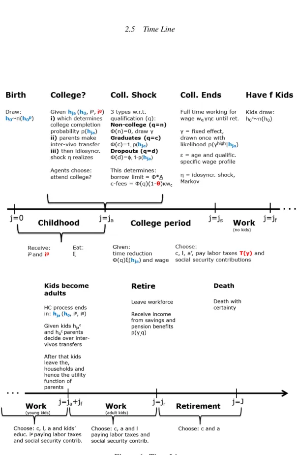
2.5 Time Line

(i) A child is born at age j = 0 with innate ability h

, drawn from a distribution that is dependent on parental innate ability, h

.

(ii) Childhood is described by ages j

, . . . , j

− 1 during which the human capital accumu-

26

Once we turn to the determination of optimal tax and subsidy policies we will treat G rather than gy as constant.

A change in policy changes output Y

and by holding G fixed we assume that the government does not respond to

the change in tax revenues by adjusting government spending (if we held gy constant it would).

lation process takes place. Parents decide on their investments into the education of their children as well as the per capita consumption of the household.

(iii) Turning j

-years old, children form an own adult household and make the college de- cision. Prior to the decision parents make inter-vivos transfers B, based on children’s acquired ability h

and innate ability h

. After these transfers have been made, children draw η from Π

(η) and make their college decision based on the state variables { j

, A = B/(1 + r(1 − τ

)), h

, h

, η}. After the decision is made non-college children (from now on households) draw the fixed e ff ect γ and start working. Households attending college draw the college completion shock, which depends on acquired human capital h

. Col- lege dropouts pay fewer college fees, face tighter borrowing limits and lower time losses from studying, all of which stands in for the shorter time period they attend college (which reflects the subperiod structure of the model at age j

for households that attend college).

Given time losses, both groups can work for non-college wages during their studies until age j

+ 1.

(iv) At age j

+ 1 college graduates and dropouts draw their productivity shock from a distri- bution contingent on qualification and acquired human capital and redraw their idiosyn- cratic income shock from a college specific distribution, η ∈ Π

(η). Ages between j

+ 1 and j

− 1 can be summarized as working without children: qualification q, productivity type γ, age-productivity profile

, and idiosyncratic shock η determine wages, w

γη

, and households face a standard labor-leisure choice in every period. This will change be- tween j

− 1 and j

when children enter the utility function.

(v) The age between j

, . . . , j

+ j

− 1 is referred to as working as parents of children. At the beginning of period j

kids enter the household and draw their innate ability based on the innate ability of parents following (8). Parents then maximize over per capita con- sumption of the household, their labor supply and their investments into their children’s human capital, i.e. i

, . . . , i

a−1

. Hence, a change of state variables takes place: par-

ent’s innate human capital is replaced by the innate human capital of their children and

acquired human capital of the child is added.

(vi) When parents are at the age of j

+ j

their children become adults. Observing the acquired human capital of their children parents transfer monetary resources B to their kids (inter-vivos transfer). Parents draw utility from the expected value function of their children at that age according to the altruism parameter ˜ ν. After that children are no longer part of parents’ value functions, implying the state space is reduced by h

and h

a

. (vii) While working as parents of adults at ages j

+ j

+ 1, . . . , j

− 1 the model reduces to

a standard consumption, labor-leisure choice model.

(viii) During retirement at ages j

, . . . , J households receive income from savings and social security p

(q, γ), which is dependent on their labor characteristics.

The timeline of the model is summarized in Figure 1.

27

The innate human capital of the child is still relevant, as its future children will draw their innate ability from

it.

Figure 1: Time Line