The Maastricht Criteria and the Euro:
Has the Convergence Continued?
Wolfgang Polasek
Christian Amplatz
The Maastricht Criteria and the Euro: Has the Convergence Continued?
ISSN: Unspecified
2003 Institut für Höhere Studien - Institute for Advanced Studies (IHS) Josefstädter Straße 39, A-1080 Wien
E-Mail: o ce@ihs.ac.at ffi Web: ww w .ihs.ac. a t
All IHS Working Papers are available online: http://irihs. ihs. ac.at/view/ihs_series/
This paper is available for download without charge at:
https://irihs.ihs.ac.at/id/eprint/1497/
The Maastricht Criteria and the Euro:
Has the Convergence Continued?
Wolfgang Polasek, Christian Amplatz
The Maastricht Criteria and the Euro:
Has the Convergence Continued?
Wolfgang Polasek, Christian Amplatz July 2003
Institut für Höhere Studien (IHS), Wien
Institute for Advanced Studies, Vienna
Contact:
Wolfgang Polasek
Department of Economics and Finance Institute for Advanced Studies Stumpergasse 56
1060 Vienna, Austria : +43/1/599 91-155 fax: +43/1/599 91-163 email: polasek@ihs.ac.at Christian Amplatz
Free University of Bozen-Bolzano e-mail: champ@dnet.it
Founded in 1963 by two prominent Austrians living in exile – the sociologist Paul F. Lazarsfeld and the economist Oskar Morgenstern – with the financial support from the Ford Foundation, the Austrian Federal Ministry of Education and the City of Vienna, the Institute for Advanced Studies (IHS) is the first institution for postgraduate education and research in economics and the social sciences in Austria.
The
Economics Series presents research done at the Department of Economics and Finance andaims to share “work in progress” in a timely way before formal publication. As usual, authors bear full responsibility for the content of their contributions.
Das Institut für Höhere Studien (IHS) wurde im Jahr 1963 von zwei prominenten Exilösterreichern –
dem Soziologen Paul F. Lazarsfeld und dem Ökonomen Oskar Morgenstern – mit Hilfe der Ford-
Stiftung, des Österreichischen Bundesministeriums für Unterricht und der Stadt Wien gegründet und ist
somit die erste nachuniversitäre Lehr- und Forschungsstätte für die Sozial- und Wirtschafts-
wissenschaften in Österreich. Die Reihe Ökonomie bietet Einblick in die Forschungsarbeit der
Abteilung für Ökonomie und Finanzwirtschaft und verfolgt das Ziel, abteilungsinterne
Diskussionsbeiträge einer breiteren fachinternen Öffentlichkeit zugänglich zu machen. Die inhaltliche
Verantwortung für die veröffentlichten Beiträge liegt bei den Autoren und Autorinnen.
to the introduction of the Euro on Jan. 1st 1999 as book currency. Defining 3 regimes, 1992- 97, 1997-1999 and 2000-2001, we analyse convergence properties, like a smooth or a rough transition in the mean or variance shifts between these 3 regimes. Given the regimes, we test the convergence in econometric models to see if the first and second moments of the convergence process are time dependent. Furthermore we check for a smooth transition process between the regimes and if the convergence process has stabilized around a target path. We find that the speed of the convergence processes for the monetary authority controlled variables (inflation and interest rates) were very different from the government controlled variables annual deficit and the public debt.
Keywords
EMU convergence, Maastricht criteria, heteroskedastic spline models, ARCH regime shifts, inflation, public deficits, interest rates and public debt
JEL Classifications
C2, E1
Comments
We thank Marco Delvai and Stefano Raffaelli for computing assistance. We also thank two anonymous
referees for the critical and valuable remarks.
1. Introduction 1
1.1 Modeling goals and caveats ... 2
2. The EMU and the Maastricht criteria 4 2.1 The Maastricht criteria ... 4
2.2 The modeling strategy ... 6
2.3 The data base... 7
3. The methodology 7 3.1 Testing in the convergence models ... 9
4. Main results 11 4.1 Inflation rates ... 11
4.2 Long-term interest rates... 15
4.3 Annual public deficit to GDP ... 19
4.4 Overall public debt ratio to GDP ... 21
5. Is there convergence in the 2
ndmoments? 26
6. Conclusions 28
References 30
Appendix: Heteroskedastic convergence models 31
1. Introduction
The EMU presently consists of 12 member states, including Greece, which joined the Eurozone in 2001, two years after the start of the new currency in 1999. The performance of the EMU countries according to the Maastricht criteria during the years before and after the formal launch of the Euro on Jan. 1
st1999 is an important threshold for a common European economic policy. With the planned enlargement of the EU, new candidates for Euro-Land will have to follow the Maastricht criteria as well. Clearly, the compliance of these prescriptions of the Pact on Stability and Growth (PSG: due to 1997) and the various discussions of these criteria are a highly political issue and are important for the future stability of the euro.
Therefore the analysis of the economic convergence process is an important issue that will serve as a benchmark for future discussion of the performance of countries in Euro-Land.
We will adopt an econometric view of the economic convergence process and we will analyze the joint time series behavior of the 4 crucial economic indicators (inflation, public deficits, interest rates and public debt) over the time period 1992-2001.
We will consider two models for the modeling of the convergence behavior over the period 1992-2001: a 2-regime and a 3-regime model. In addition, we will consider a smooth spline model and a piecewise regression model where the pieces might not be connected. The spline model preserves continuity at the break point while the piecewise regression model describes the trend lines independently in two or 3 regimes.
The description of the convergence process is a simple time trend model that could possibly have quite different trends in the consecutive regimes. The 3-regime model introduces a second break point at the end of 1999 to describe the performance of the last two years. We will test the convergence of the spline and the piecewise linear regression model.
Furthermore, we distinguish between the following types of convergence processes:
a) Simple mean convergence: The cross-sectional means of the time series are decreasing.
b) Targeted mean convergence: The cross-sectional means of the time series are decreasing to a target level and the cross-sectional variance of the process is also decreasing.
c) Simple variance convergence: The cross-sectional variances of the time series are decreasing.
Simple mean (or variance) divergence: The cross-sectional means (or variances) of the time
series are increasing.
1.1 Modeling goals and caveats
Clearly, our approach is merely an ex-post statistical measurement of the observed movement in the underlying time series for the Maastricht Criteria of the EU countries. Since no behavioral assumptions are present in our econometric models, we concentrate on and describe the phenomenon of convergence in a statistical sense. A driving role for the convergence process is played by expectations and policy credibility, which are rather complicated to impose in a descriptive approach and therefore are not considered explicitly in this paper.
Economically, we expect from the results that modeling the convergence process of inflation and long-term interest rates on the one side and annual deficits on the other side can be quite different. While the criteria for inflation and long-term interest rates were considered to be a strict entrance benchmark for the EMU, the criterion for government finances was less restrictive. Governments who had the intention to meet the government finance criteria were considered to be eligible for Euroland, too.
We expect that inflation and interest rates, two of the convergence criteria, will have similar convergence behavior because of their close economic interrelationship. Indeed, for several models inflation depends on the exogenously given level of nominal interest rates (e.g. see Dornbusch 1976). On the other hand Central Banks, especially the ECB (see Treaty on EU (1999), articles 105-124), set the level of nominal interest rates according to inflationary pressure. Moreover, debt ratios and annual deficits also are interrelated. On the other hand, convergence performance of these two groups of criteria is not necessarily related to each other, especially not in the beginning of the convergence procedure, i.e. in our notation for the Maastricht regime. The reason for this is that fiscal convergence is driven by business cycles and fiscal discipline.
Fiscal discipline, though, has certainly improved in the Eurozone by the PSG. Unfortunately, the problem of business cycles affecting government budgets was not taken into account by the PSG, since it focuses on annual deficits instead of business cycle independent structural deficits. This shows certain weaknesses of the two fiscal Maastricht criteria and the PSG.
Thus there is possibly room for improving rules of the PSG in the future.
Furthermore, we argue that the PSG is not necessarily satisfactory, neither for guaranteeing
stabilization of achieved convergence of interest rates and inflation nor for implementing a
consistent long-term trend towards perfect convergence of the Maastricht criteria nor for
necessarily achieving economic convergence. The reason is that the PSG may create
incentives for fiscal discipline and thus for fiscal convergence, but it does not necessarily
imply economic convergence (e.g. in the sense of similar income levels or growth rates) nor
convergence in the sense of converging interest rates and inflation.
Still concerning the PSG, we conclude that there is a principal-agency problem. Indeed, member countries have fewer incentives for further improving or at least stabilizing convergence, once they joined the Euro. Thus there is some evidence for divergence in the Euroland regime concerning several criteria. This is consistent with the hypothesis that the concept of convergence is highly time dependent. In fact we conclude that different time periods may show totally different convergence performance.
Greece is treated as a special case in this paper because of its different economic stage compared to other EMU members. Analysis without Greece deals with the fact of its being an outlier, but at the same time it allows classifying the convergence performance of Greece when comparing to results including Greece. In this sense Greece is somewhat like a pioneer for the coming eastern enlargement. Once the “eastern enlargement” of the EU has taken place, discussion about the adoption of the Euro in those new member countries will arise.
Furthermore we are interested in the question if the convergence process in the first moments (i.e. the mean equation of the spline model) was accompanied by a convergence process in the 2
ndmoments. This means that we fit a heteroskedastic 2- or 3-regime convergence model for the conditional variances of the piecewise regression models.
Thus, it is not surprising that after the introduction of the Euro not all the countries fulfill the restriction of the maximum 60% debt to GDP ratio: 5 and 6 countries are not able do so in 2000 and 2001 respectively. We will see that the convergence for inflation and interest rates, – these are the two criteria depending on efficient financial and goods and services markets – already took place in the first regime before 1997. This is a clear indication that real economic convergence can be achieved more quickly than fiscal discipline for the public sector.
We also want to emphasize that the proposed convergence model is motivated by the econometric technique of spline models and has nothing to do with the approaches to economic convergence as in Barro et al. (1995) or Ben-David (1993). Different ideas regarding economic convergence by index construction can be found in Hobijn and Franses (2000, 2001).
The plan of the paper is as follows: We start in section 1 with an introduction to the modeling
process; the data base and the Maastricht criteria are described in section 2. In section 3 we
briefly outline our econometric convergence approach while in section 4 we report the
results. Section 5 reports the results of the heteroskedastic convergence models. The last
section concludes. The appendix summarizes the heteroskedastic convergence models.
2. The EMU and the Maastricht criteria
First, let us consider a short historical overview of the EMU. The Maastricht treaty laid out three stages to arrange the EMU:
Stage 1, July 1990 – Dec 1993:
• Free movement of capital,
• Narrowing of ERM band,
• Closer co-operation between central banks,
• Closer co-ordination of economic policies.
Stage 2, Jan. 1994 – Dec 1998:
• Convergence of member states' economic and monetary policies,
• Establishment of European Central Bank,
• Independence of national banks,
• Participating countries fix their exchange rates.
Stage 3, Jan. 1999: Introduction of the Euro as a book currency,
• Jan. 2002: Launch of euro notes and coins.
In 1998, 11 of the 15 EU member states decided to form the European monetary union (EMU), leaving Denmark, Greece, Sweden and the UK outside the “eurozone”.
In January 1999, financial markets of the EMU countries began operating in euros. Two years later, Greece finally met the economic requirements for membership and at the Lisbon meeting in June 2000 Greece was allowed to join the euro in January 2001.
2.1 The Maastricht criteria
We consider the twelve countries belonging to the European Monetary Union (EMU):
Germany, France, Belgium, Luxembourg, Austria, Finland, Ireland, the Netherlands, Italy, Spain, Portugal are the founding states and Greece joined two years later. The other three EU states, Britain, Denmark, and Sweden have not joined the Euro.
The Maastricht Treaty (1992) contains important macro-economic requirements in order to
become a member of Euroland, i.e. to participate in the EMU. The treaty lists 4 types of
criteria that are slightly different from the 4 “Maastricht” criteria, which we will use for the analyses of the convergence process. The 3
rdpoint mentioned in the treaty deals with exchange rates, but this was only important before the official launch of the Euro on Jan. 1
st1999. Therefore we have not considered exchange rates for the present analysis, and we investigate the behavior of government budgets – according to common practice – by two important time series, the annual deficit and the debt ratio.
1. PRICE STABILITY
"The achievement of a high degree of price stability [...] will be apparent from a rate of inflation which is close to that of, at most, the three best-performing Member States in terms of price stability."
In practice, the inflation rate of a given member state must not exceed the inflation rate of the three best-performing member states in terms of price stability during the year preceding the examination of the situation in the given member state by more than 1½ percentage points.
2. GOVERNMENT FINANCES
"The sustainability of the government financial position [...] will be apparent from having achieved a government budgetary position without a deficit that is excessive [...]."
In practice, the Commission, when drawing up its annual recommendation to the Council of Finance Ministers, examines compliance with budgetary discipline on the basis of the following two criteria:
a) The annual government deficit: the ratio of the annual government deficit to gross domestic product (GDP) must not exceed 3% at the end of the preceding financial year.
If this is not the case, the ratio must have declined substantially and continuously and reached a level close to 3% (interpretation in trend terms) or, alternatively, must remain close to 3% while representing only an exceptional and temporary excess;
b) Government debt: the ratio of gross government debt to GDP must not exceed 60% at the end of the preceding financial year. If this is not the case, the ratio must have sufficiently diminished and must be approaching the reference value at a satisfactory pace (interpretation in trend terms).
3. EXCHANGE RATES
"The observance of the normal fluctuation margins provided for by the exchange-rate
mechanism of the European Monetary System, for at least two years, without devaluing
against the currency of any other Member State."
This criterion is not relevant for this study, as we only look at the performance of countries already being members with a common currency.
4. LONG-TERM INTEREST RATES
"The durability of convergence achieved by the Member State [...] being reflected in the long- term interest-rate levels."
In practice, the nominal long-term interest rate must not exceed that of the three best- performing Member States in terms of price stability by more than 2 percentage points. Note that this refers to the same Member States as in the case of the price stability criterion. The crucial period is the year preceding the examination of the Member State for joining the euro.
Therefore we will focus our analysis on the inflation rates, the nominal long-term interest rates, annual government deficits and total public debt of each member, while simply ignoring the criterion regarding exchange rates, as it is obsolete now.
2.2 The modeling strategy
The empirical strategy employed in the paper implicitly assumes that there is a common (across member states) 'generating mechanism'. The implicit assumption is a common cross-sectional time trend according to Quah (1993). According to this view, our modeling proposal considers the fact that the time series do not follow a uniform linear trend but perhaps a broken, segmented, possibly piecewise connected (“smooth”) trend. For each Maastricht criterion we will estimate a convergence model across the 12 EMU members and results of the convergence performance will be obtained independently for the four variables.
We will treat the convergence modeling as a model selection problem: We look for the best performing parsimonious convergence model. Thus, this approach requires many estimates because different piecewise linear regression models have to be compared to each other.
Furthermore, we have to cope with outliers? exceptions, since Greece in particular is a special case for the convergence models. Greek time series can be considered to document a previous unseen catching-up process and therefore it is not surprising that Greek time series are “outliers” in the sense of showing more extreme values in the first years of the convergence process if compared to other countries.
Unfortunately, from an econometric point of view, the Greek time series create a technical
difficulty in the assumption that the convergence process in the Maastricht regime stems
from a data generating process of the EU countries, which is “uniform”. That means they
agree at the same time to similar economic policy measures, they have the same time
horizon to meet their goals, and they have roughly comparable starting conditions. Therefore
the fact that Greece entered the EMU in 2001, after the introduction of the Euro by the other
countries, distorts the estimation of the convergence process (due to a single country) and has an “outlier bias” effect on the least squares estimates.
To find out how big this effect of distortion can be on the estimates, we will analyze the convergence in our models without Greece (and occasionally without other “outlying”
countries) to see its influence on the overall convergence behavior. Furthermore, we will check the analysis of overall public debt for outlying countries. As Luxembourg, Belgium, Italy and Greece all show extreme debt values compared to the other 8 countries (i.e.
Luxembourg has a very low one, the other three a very high one), we will estimate the regression model for the group of 8 middle or “core“ countries.
2.3 The data base
Data for EMU members are taken from Eurostat on a monthly or a yearly basis. The inflation rate is calculated from the price index (source: Datastream, IMF) from Sept. 1991 to Sept.
2001. For the interest rates we had to start the convergence analysis in April 1994 since the data were not available or comparable before 1994. The long-term interest rate for each country is the “Benchmark Bond 10 yr (DS)”.
The monthly time series on the interest rate and the inflation were available up to September 2001. Finally the annual time series on annual deficit to GDP and overall public debt to GDP are based on OECD forecasts for the year 2001, since they are the only annual data sets that are available.
After calculating the mean of the three best performing countries for inflation rates each month, we subtract it from all national inflation rates for comparative purposes. The same procedure is applied to interest rates. Data for annual and overall public debt are all in absolute percentage terms to GDP. They are due to an OECD database for forecasts, annual reports of the European Central Bank for 1998 to 2000 and Eurostat, covering the years from 1990 to 1997. These data sets for the four criteria are sufficient for our research objective.
3. The methodology
To find out whether the convergence process of the Maastricht treaty has not eroded but
continued in the two years since the introduction of the Euro, we suggest to model the
convergence path for the EMU member states over the last decade by a piecewise
regression model. By looking at the graphs of the individual time series for the convergence
models, it is quite evident that there was an important change in the convergence process at
the end of 1997. Indeed, there was a European Council meeting in Amsterdam on June 17
th1997, which agreed on the so-called Pact of Stability and Growth (PSG). This political
decision made clear that the admittance of countries into Euroland would be based on hard economic facts. The pact enforces also the fulfillment of EMU criteria over the next years.
Maybe it was not as important as the Maastricht Treaty (1992) was, but it provided market participants with really strong expectations for convergence to take place. We will show, though, that the convergence for inflation and interest rates of EMU members, which are the two criteria depending on efficient financial and goods & services markets, already approached a similar level in member countries before. This may partly be due to real economic convergence already starting before and partly due to expectations of market participants already anticipating real events.
Our convergence modeling is based on a separate and a continuous piecewise linear regression model for a pooled cross-section and time series data set. We first introduce the so-called continuous piecewise regression or spline model (see e.g. Pindyck and Rubinfeld, 1998) using dummy variables for the known break point x* which is assumed at the end of 1997.
The 2-regime spline model is given by
(1) y
t= b
0+ b
1x
t+ b
2(x
t– x*)D
t+ u
t, Var (u
t) = s
2, whereby the dummy variable is defined as
(2) D
t= 1 for x
t> x* and D
t= 0 else (for x
t< x*).
This leads to the two regression lines before and after the break point x* which has the property that
D
t= 0: y
t= b
0+ b
1x
t+ u
t, for x
t< x*, D
t= 1: y
t= b
0* + b
1* x
t+ u
t, for x
t> x*,
The coefficients for regime 2 are b
0* = b
0– b
2x* and b
1* = b
1+ b
2.
The 2-regime separate regression model has the form of a regression model with a
“multiplicative dummy” variable where we use the regressor x
t– x*:
(3) y
t= b’
0+ b
1(x
t– x*) + a
0D
t+ a
1(x
t– x*) D
t+ u
t, Var (u
t) = s
2,
In this model the regressor variable x
t– x* = t – t* is the break point adjusted time variable
and it shifts the coordinate system into the break point t*. Therefore a
0and b’
0are the
intercepts of the two independent trends while a
1and b
1are the slopes of the two regimes.
The 2-piece separate regression model (3) is the unrestricted model and it contains the 2- regime spline model (1) as special case. Therefore the hypothesis of a continuous trend can be tested if the coefficient a
0= 0, i.e. a simple t-test.
The 3-regime separate regression model has the form
(4) y
t= b
0+ b
1(x
t– x
a*) + a
0D
at+ a
1(x
t– x
a*) D
at+ c
0D
ct+ c
1(x
t– x
c*) D
ct+ u
t, Var (u
t) = s
2.
D
atis the dummy variable for the regime A, i.e. D
at= 1 for x
t> x
a* and D
at= 0 else; and D
ctis the dummy variable for the regime C, i.e. D
ct= 1 for x
t> x
c* and D
ct= 0 else. Now x
a* is the known break point for the regime A and x
c* is the known break point for the regime C.
Maastricht regime Amsterdam regime Euroland regime
|_______________________|___________________|___________________|
t = 1 97M12 = x
a* 99M12 = x
c* t = T
regime: A B C
Scheme 1: The regimes for testing the convergence model
One break point x
a* is only needed to estimate the two-regime model while two break points x
a* is x
c* are needed to estimate the 3-regime spline model. The first break point is assumed to be December 1997 as 1997 was the crucial year for the final decision on the countries that were allowed to adopt the Euro. This decision on the EMU was to be made in the middle of 1998 after the 1997 data for the convergence criteria being available. The second break point x
c* marks the starting point of the Euro as a book currency, and we choose for data compatibility reasons December 1999. We will call the first regime the “Maastricht regime”
and the second regime until the end of 1999 when the Euro was created as the “Amsterdam regime”. The third regime is the “Euroland regime”.
3.1 Testing in the convergence models
We will test the following 4 hypotheses for the piecewise regression models (continuous or separate):
Hypothesis 1: The EMU countries have reached convergence in the Maastricht regime.
Then the pooled trend coefficient has to be negative (and the intercepts should be positive).
If countries had had no interests in the Maastricht convergence process then on average
they would have maintained their old economic policy and the pooled trend coefficient would
be zero. This leads to the one-sided hypotheses that the countries have not reached convergence as being the null-hypothesis, and the hypotheses
H
0: b
1= 0 vs. H
1: b
1< 0.
Hypothesis 2: The EMU countries have stabilized the convergence process in the Amsterdam regime.
This implies a simple t-test for the slope coefficient in the 2
ndregime:
H
0: b
1* = 0 vs. H
1: b
1* ≠ 0.
Hypothesis 3: The EMU countries have not diverged in the Euroland regime.
Again, this implies a one-sided t-test for the slope coefficient in the 3
rdregime:
H
0: b
1* = 0 vs. H
1: b
1* > 0.
In contrast to the separate 3-regime regression model in (4) we can estimate the 3-regime continuous spline model:
(5) y
t= b
0+ b
1(x
t– x
a*) + a
1(x
t– x
a*) D
at+ c
1(x
t– x
c*) D
ct+ u
t, Var(u
t)= s
2,
Therefore we compare the separate 3-regime regression model with the continuous spline model by an F-test on:
Hypothesis 4: The EMU countries have stabilized convergence in the Amsterdam and the Euroland regime in a continuous way (smooth transition).
The compound hypothesis is that the restricted model holds:
H
0: a
0= 0 and c
0= 0 vs. H
1: a
0≠ 0 or c
0≠ 0 .
A smooth transition is preferred if the spline model is more likely than the piecewise 3-regime
model. Instead of the F-test we can also use a likelihood ratio test or we simply compare the
models by information criteria like AIC (Akaike 1973), or the Schwartz criterion. Thus, our
approach tries to find stylized facts in the spirit of a critical empirical analysis as proposed by
Popper (2000).
Hypothesis 5: The EMU countries have achieved a) convergence also with respect to the variance in the Maastricht regime and b) have not diverged in variance during the Amsterdam and Euroland regime.
Let α
time, β
timeand γ
timebe the coefficient of the TIME variable in the variance equation of the 3-regime ARCH regression model (see appendix), then the two hypotheses imply:
a) H
0: α
time<= 0 vs. H
1: α
time> 0 ; b) H
0: β
time= γ
time= 0 vs. H
1: β
time= γ
time≠ 0.
We shall denote a convergence process in a certain regime a “targeted convergence” if the TIME coefficients in both, the mean and the variance equation, are significantly different from zero and negative. If the regime dependent TIME coefficients are positive then the process is called in this regime divergent. If the TIME coefficients are not significantly different from zero then there is no convergence (or divergence) for the given partition of the process into regimes.
In the next section we report the main results of the convergence models.
4. Main results
In the following section we compare the estimation results of different convergence models for each Maastricht criterion.
4.1 Inflation rates
The estimates for the 2-regime spline regression that includes all the 12 members are (values within brackets are p-values):
Before 98M1: Infl.differential = 3.175 – 0.029*Time
(p-values) (0.0000) (0.0000)
After 97M12: Infl.differential = 0.773 + 0.002*Time
(p-values) (0.0001) (0.0000)
On average the inflation differential in Euroland with respect to the mean of the three best
performing countries decreased from 3.17 % to only 0.96% at the end of 1997 (about 3 basis
points per month). Surprisingly, there was no continued convergence in the second
Amsterdam regime. Since the regression coefficient is positive there was actually a small divergence, namely 0.2 basis points per month with the inflation rate differential increasing to 1.08% at the end of the second regime. Regression estimates are all significantly different from 0 (p-value = 0.0001).
Since Greece data behave like those of outlying countries/non-members, we have estimated the 2-regime model for 11 EMU countries.
Before 98M1: Infl.differential = 1.960 – 0.017*Time (p-values) (0.0000) (0.0000) After 97M12: Infl.differential = -0.047 + 0.010*Time
(p-values) (0.0000) (0.0000)
The estimates for the 11 countries show a lower pace of convergence (1.7 basis points compared to 2.9 per month) in the first regime. Again, we see a divergence of 1 basis point for the second regime which is considerably higher than for the first regime. The differential is 1.96% for September 1991, 0.68% for December 1997 and 1.11% for September 2001.
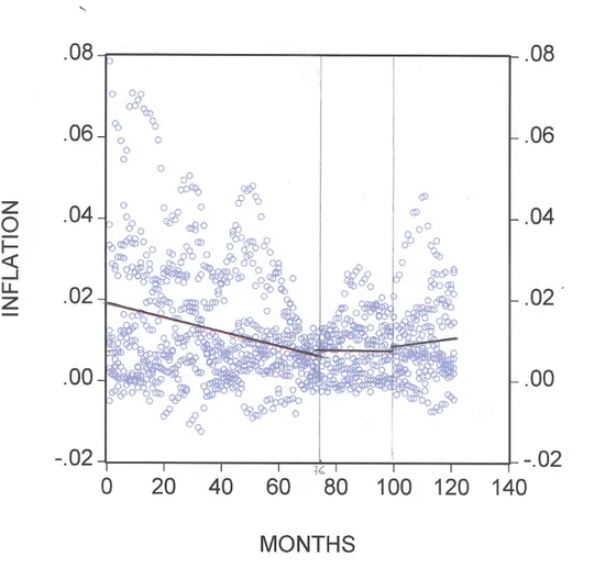
Next we want to check if the divergence process has continued for the 3
rdregime in Euroland between 2000 and 2001 (again without Greece) without Greece:
Before 98M1: Infl.differential = 1.956 – 0.017*Time
(p-values) (0.000) (0.000)
From 98M1 to 99M12: Infl.differential = 0.063 + .008*Time
(p-values) (0.000) (0.010)
After 99M12: Infl.differential = -0.392 + 0.013*Time
(p-values) (0.000) (0.7676)
While the slope coefficient in the 3
rdregime is not significant, the positive slope in the 2
ndregime is. This can be seen as the result of an increased spread in the inflation rates in the
Euroland regime. Note that hypothesis 3, i.e. the divergence of countries during the Euroland
regime, cannot be confirmed significantly by the t test.
Figure 1: Inflation differential for the 3-regime spline model (break points at 97M12 and 99M12) without Greece
Finally we test the hypothesis that the transition between the regimes was smooth for the inflation rates. The separate 3-regime model is estimated as:
Before 98M1: Infl.differential = 1.973 – 0.017*Time
(p-values) (0.000) (0.000)
From 98M1 to 99M12: Infl.differential = 0.589 + 0.003*Time
(p-values) (0.1915) (0.0970)
After 99M12: Infl.differential = -0.696 + 0.016*Time
(p-values) (0.1014) (0.0267)
Figure 2: Inflation differential for a separate 3-regime regression for 11 EMU countries
The estimates are rejecting the convergence hypothesis for the last regime and the 1.6 basis points divergence is significant. Moreover, note the divergence for the years 1998 and 1999.
Indeed, the slope coefficient is significantly different from 0 (α = 10%) and the F-test is significant as well (p-value < .0001).
Concerning the third hypothesis about the number of regimes, we see a clear preference for
the 3-regime model. (The AIC value for the 3-regime model is –5.884 while the AIC value for
the 2-regime model is –4.660). The likelihood ratio test between the 2 models is highly
significant, too. This means that the whole convergence process happened in the Maastricht
regime while the stabilisation process for the Amsterdam and the Euroland regime is quite
different.
For the 4
thhypothesis about the smooth transition we find almost identical AIC and log- likelihood values for both models. Therefore we will prefer the smooth transition model according to the principle of parsimony (i.e. the smallest number of parameters).
Conclusion 1: The convergence for the inflation rate in the EMU countries happened statistically significant during the Maastricht regime. For the 2
ndregime and the 3
rdregime we find a flat regression line (i.e. a levelling off) and the smooth transition model is supported by the data. From January ‘00 to September ’01 we detect a small but non-significant divergence between the inflation rates.
4.2 Long-term interest rates
The 2-regime spline model for the 12 EMU members is estimated as:
Before 98M1: Int.differential = 2.990 – 0.048*Time (p-values) (0.0000) (0.0000) After 97M12: Int.differential = 1.500 – 0.015*Time (p-values) (0.0000) (0.0015)
Thus, from April 1994 to December 1997, the monthly convergence was on average 4.8
basis points. The long-term interest rate differential – based on the mean of the three best
performing countries – has on average decreased from 3% to 0.8% at the end of the first
regime, 1997. There has been additional convergence for the second regime of 1.5 basis
points with the differential decreasing to quite a low value: less than 0.2%. The results are all
significant at a 1% level (including the F-statistic).
Figure 3: Convergence of the interest rate differential in the 2-regime spline model (of 12 EMU countries). The time series of Greece acts as an outlier. Note the bias of the trend in the second regime due to Greece.
The spline estimate without Greece is:
Before 98M1: Int.differential = 2.200 – 0.045*Time
(p-values) (0.0000) (0.0000)
After 97M12: Int.differential = 0.220 – 0.001*Time
(p-values) (0.0000) (0.0000)
The 11 countries of Euroland show a good convergence trend (4.5 basis points per month)
for the interest rates in the first regime. The convergence has stabilized over the last 2
regimes, and seemed to have been more constant than for the inflation rates. The estimated
differential with respect to the 3 best performing countries is 2.2% for April 1994, 0.2% for
December 1997 and about 0.15% for September 2001. As only the latter value is similar to
that of the regression including Greece, this shows the size of the distortion effect, although it is vanishing over time.
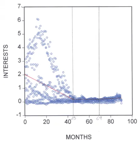
The 3-regime spline model (again without Greece) was estimated as:
Before 98M1: Int.differential = 2.177 – 0.043*Time (p-values) (0.0000) (0.0000)
From 98M1 to 99M12: Int.differential = 0.535 – 0.007*Time (p-values) (0.0000) (0.0000)
After 99M12: Int.differential = -0.585 + 0.009*Time (p-values) (0.0000) (0.2016)
The slope coefficient is (statistically) significant in the second regime but not so for the 3
rdregime. Practically the convergence process for the interest rates has already been flat in the 2
ndregime and has stabilized in the 3
rdregime. Clearly, the variance reduction is impressive for the Maastricht regime, as we see from Figure 4.
Figure 4: The 3-regime spline convergence model for interest rate differentials
The estimation for the separate 2-piece linear regression model without Greece is:
Before 98M1: Int.differential = 2.151 – 0.042*Time
(p-values) (0.0000) (0.0000)
From 98M1 to 99M12: Int.differential = 0.176 – 0.001*Time
(p-values) (0.0005) (0.0001)
After 99M12: Int.differential = -0.519 + 0.009*Time
(p-values) (0.0047) (0.0000)
Figure 5: Separate regression for the interest rate differential (breaks points at
97M12 and 99M12) without Greece
Now to the question: which model is preferred, the 2- or the 3-regime model? As with the inflation rate model, we see a clear preference for the 3–regime model. The AIC value for the 2-regime model is 2.888 while the AIC value for the 2-regime model is 4.346, and the likelihood ratio test is highly significant. (The difference of the log-likelihoods is about 150 which is distributed as a chi-square variable with 1 d.f., the difference of the numbers of parameters between model (2) and (5)). We find an impressive convergence process for the inflation rates during the Maastricht regime (see last section) that was matched by a similar process for the interest rate differentials. Note that the stabilization process for the Amsterdam and the Euroland regime is quite similar. While the slope of the 2
ndregime was slightly negative, it became positive in the 3
rdregime, although both slopes are non- significant. Concerning hypothesis 4 about the smooth transition, we find again almost identical AIC and log-likelihood values for both models. (The AIC value is 2.892). Thus, we prefer the smooth transition model for the interest rates convergence.
Conclusion 2: The convergence for long-term interest rates in the EMU for the first two regimes was similar to the convergence process of the inflation rates and has leveled off in the last two regimes from January ‘98 to September ’01. The smooth transition model is preferred by the data, and a slight divergence effect in mean and variances can be seen for the last regime.
4.3 Annual public deficit to GDP
The analysis for the annual public deficit is based on annual data. This implies shorter time series and the estimation of a 2-regime model, i.e. we will mainly learn about the convergence process before and after 1997. Because of pooling the data, we have enough d.f. to estimate a 2-regime model, but these yearly estimates are less reliable and interpretable than quarterly results. The spline estimates are
Before 1998: Ann.Deficit = 5.31% – 0.30%*Time
(p-values) (0.000) (0.0303)
After 1997: Ann.Deficit = 12.26% – 1.17%*Time (p-values) (0.000) (0.0134)
We see that the EMU countries reduced their annual deficits with an annual rate of 0.3%-
points (p-value = 0.0303). In the second regime the trend was even more evident (-1.2% per
year with a p-value of 1.3%). The estimated regression line crosses the 3% target line in
1997.
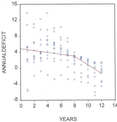
Figure 6: Spline model of the annual deficit for the 11 EMU members
2-regime regression estimates without Greece for the annual deficit:
Before 1998: Ann.Deficit = 4.35 – 0.21*Time,
(p-values) (0.000) (0.0994)
After 1997: Ann.Deficit = 11.52 – 1.10*Time.
(p-values) (0.000) (0.0063)
The slope in the first regime is flatter than before and is only significant at a 10% level. This
means that the hypothesis for non-convergence during the Maastricht regime cannot be
rejected. The estimated regression line again crosses the 3% line in 1997. In the second
regime the negative trend is significant, irrespective of Greece being included or not. This
means that the EMU countries started seriously reducing their annual deficit only in the last
regimes since 1997. The F-value is highly significant at a .001% level. Note that the general
trend has changed for most countries in the last regime, since all countries were still below the 3% line for their projected annual deficit in 2001.
Conclusion 3: On average the EMU members have decreased their annual public deficit (ratio to GDP) over the whole period since 1992. Before 1997, in the Maastricht regime, the reduction of the deficit was not statistically significant and in addition, no convergence in the variances can be seen. Since 1997 the time trend in the means is significant and the variance is smaller than in the Maastricht regime.
4.4 Overall public debt ratio to GDP
Finally we test if EMU members have decreased the overall public debt ratio on average in 2000 to 2001. The linear spline model including all the 12 members is estimated as:
Before 1998: Debt = 63.48 + 1.45*Time (p-values) (0.000) (0.2815) After 1997: Debt = 105.34 – 3.78*Time
(p-values) (0.000) (0.1315)
We see that convergence will not take place in the first regime: on the contrary, we see an increase of the overall public debt ratio for regime 1, on average with an annual rate of 1.45%. But this coefficient is not statistically significant (p-value = 0.2815), and in the second regime the countries tend to decrease their debt levels by 3.8% per annum; but the slope coefficient is also not significant: p-value = 13.15%. Since only 12 annual observations are available, this small number of observation can explain this low empirical evidence, i.e.
leading to insignificant results. Interestingly, the estimated regression line reaches the 60%
level at the end of our observation period in 2002.
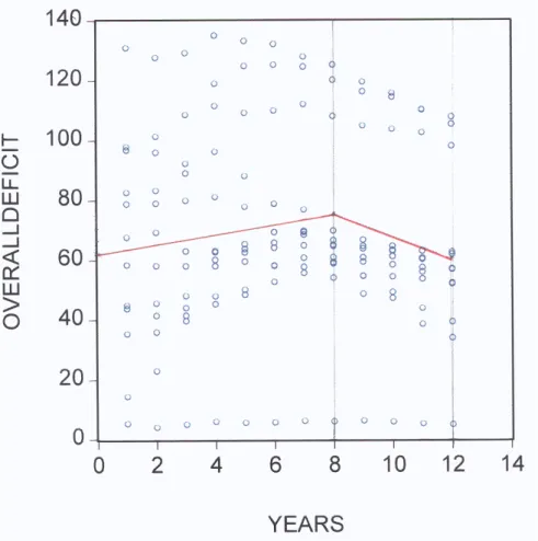
Figure 7: 2-regime spline model of the overall public debt ratio (12 EMU members)
The estimates of the 2-regime spline model for public debt (excluding Greece) are:
Before 1998: Debt = 61.86+1.20*Time (p-values) (0.0000) (0.3891) After 1997: Debt = 101.22-3.72*Time
(p-values) (0.0000) (0.1712)
All estimates and p-values do not change substantially from the previous regression
including Greece and the fit has not improved.
Figure 8: 2-regime model of the overall public debt for (11 EMU countries without Greece)
In order to find a significant trend model we have excluded those countries which might influence average behavior through extreme values. Such a country is Luxembourg because of its low debt ratios (see Figure 8), and Belgium, Italy and Greece with high debt levels on the other side. Thus we estimate the aggregate convergence model for the remaining 8
‘middle’ countries:
Before 1998: Debt = 55.57 + 1.25*Time
(p-values) (0.000) (0.0770)
After 1997: Debt = 94.95 – 3.67*Time
(p-values) (0.000) (0.0076)
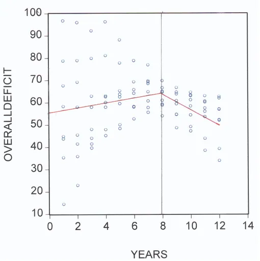
For these 8 countries the debt increases 1.25% annually (the p-value is 10%) during the first regime until 1997, the F-test is significant. The estimated debt in 1997 is about 65.5%, which is above the 60% ceiling target. The level was at 55.6% in 1990, therefore we see a divergence until 1997 but a significant debt decreases of 3.7% annually over the second regime. Therefore the estimated regression line for the 8 countries crosses the 60% line in 1999. This means that the 8 countries maintain the trend of reducing their annual deficit until 2002 with an estimated value of 50.9%.
Figure 9: Overall public debt for the ‘middle’ EMU members (without Belgium, Luxembourg, Greece and Italy)
Conclusion 4: The convergence analysis for annual debts reveals the most heterogeneous
behavior: during the Amsterdam regime until 1997 the debt ratio was slightly but not
significantly increasing for 8 “core” countries. Since 1997 the trend is significantly decreasing
for the remaining 4 countries, too. Overall, after a flat start during the Maastricht regime, a
general trend of reducing national debts since 1998 can be observed, which continued in
2000 and 2001.
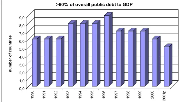
Additionally, the number of EMU members not meeting the 60% target on the overall public debt ratio has decreased in 2000 and 2001. Figure 10 shows a steadily decreasing number since 1996, particularly in 2000 and 2001. While there were 9 countries exceeding the 60%
ceiling in 1996, only 7, 6 and 5 did so for 1999, 2000 and 2001 respectively. This is a sign for a small improvement of the debt ratio, but the evidence for a rigorous debt convergence remains weak since all countries are required to have a debt ratio lower than 60%.
0,0 1,0 2,0 3,0 4,0 5,0 6,0 7,0 8,0 9,0
number of countries 1990 1991 1992 1993 1994 1995 1996 1997 1998 1999 2000 2001p