O R I G I N A L P A P E R
Risk, time pressure, and selection effects
Martin G. Kocher1,2• David Schindler3•Stefan T. Trautmann3,4 • Yilong Xu4
Received: 18 July 2017 / Revised: 26 April 2018 / Accepted: 2 May 2018 ÓThe Author(s) 2018
Abstract Time pressure is a central aspect of economic decision making nowadays.
It is therefore natural to ask how time pressure affects decisions, and how to detect individual heterogeneity in the ability to successfully cope with time pressure. In the context of risky decisions, we ask whether a person’s performance under time pressure can be predicted by measurable behavior and traits, and whether such measurement itself may be affected by selection issues. We find that the ability to cope with time pressure varies significantly across decision makers, leading to selected subgroups that differ in terms of their observed behaviors and personal traits. Moreover, measures of cognitive ability and intellectual efficiency jointly predict individuals’ decision quality and ability to keep their decision strategy under time pressure.
Keywords RiskCognitive abilitySelectionTime pressure
JEL Classification C91D81
& Stefan T. Trautmann
trautmann@uni-hd.de
1 University of Vienna, Josefstaedter Str. 39, 1080 Vienna, Austria
2 IHS Vienna, Vienna, Austria
3 Department of Economics and CentER, Tilburg University, P.O. Box 90153, 5000 LE Tilburg, The Netherlands
4 Alfred-Weber-Institute for Economics, University of Heidelberg, Bergheimer Str. 58, 69115 Heidelberg, Germany
https://doi.org/10.1007/s10683-018-9576-1
1 Introduction
Many, if not most, decisions in the workplace are made under time pressure today (Reid and Ramarajan 2016; Wheatley 2000). Consequently, research in decision making has recently started to investigate how a time constraint influences individuals’ preferences and choices (for an overview, Spiliopoulos and Ortmann 2017). By randomly allocating subjects into time pressure conditions, the literature has successfully identified its causal effects in a variety of domains, including risky, social, and strategic behavior (e.g., Sutter et al.2003, on bargaining; Kocher and Sutter2006, on beauty contests; Baillon et al.2013, on decisions under ambiguity;
Kirchler et al.2017, on risky decisions; Buckert et al.2017, on imitation in strategic games; Haji et al.2016, on bidding in auctions).
However, these causal effects should be interpreted with caution, because of two potentially serious problems, both relating to issues of self-selection. First, because people differ in their ability to cope with time pressure (e.g., Claessens et al.2017;
Eisenhardt1989; Maruping et al.2015, and references therein), we expect people self-select into decision environments with a different degree of time pressure. That is, outside the experimental laboratory, candidates self-select into activities and occupations and thus into job-related decision-making environments. In contrast, participants in experiments are exogenously assigned to treatment conditions that may not fit well with their tastes and skills (Omar and List2015). External validity of the observed experimental behavior thus cannot be taken for granted. Despite similarity of the experimental and the natural decision environments (in term of time pressure), the decision makers may systematically differ across the two settings in a self-selected way. Importantly, while external validity is an issue in any empirical study, it is a more central aspect in laboratory experiments that explicitly aim to mimic natural decision environments.1Understanding the personality traits associated with the ability to perform under time pressure in the lab would allow an assessment of such selection in the field, and thus of the external validity of (lab- measured) average causal effects based on the distribution of traits in actual decision environments. Identifying such traits is one aim of the current paper.
Second, if time pressure is substantial and relevant in an experiment, some people will violate the time constraint. This leads to problems of the internal, rather than the external validity of the time pressure effects, because the sample of decisions observed in the data set is self-selected.2Failure to take these selection effects into account may therefore result in a false interpretation of the observed behavior in terms of population averages. For example, Tingho¨g et al. (2013) argue that failures to replicate time pressure effects on cooperation in ethical dilemmas (Rand et al.2012) may be due to the original studies excluding about half of the participants because of a failure to meet the time constraint (Casari et al. (2007) make a similar observation in the context of auction bidding; Ambuehl et al. (2018)
1 External validity may be less of a problem in other contexts, for example time-limited offers to consumers (Sugden et al.2015), where self-selection is less likely.
2 A similar problem exists in studies on the effect of stress on decision making, where analyses of data are typically restricted to those participants who show a cortisol reaction under stress (Trautmann2014).
show how high incentives disproportionally lure cognitively disadvantaged agents to self-select into transactions of unclear consequences).
The current study aims to shed light on such heterogeneity and the resulting selection effects in the presence of exogenously imposed time pressure. To this end, we separately analyze subsamples of subjects who fail, respectively succeed, to react in time, in terms of their behavior and traits. We demonstrate that overlooking the selection issue in this context would result in a very different assessment of the performance under time pressure. We focus on the domain of risky decisions. In
‘‘Risky behavior under time pressure: summary of results’’ in ‘‘Appendix’’, we review the findings of the experimental literature in this domain. We indicate for each study whether there is a potential threat to internal validity because of substantial violations of the time constraints, or whether there is low time pressure, questioning relevance. Table8 in ‘‘Appendix’’ suggests that selection problems should be taken seriously in the interpretation of causal time pressure effects on risk taking.
Observing that selection issues are at the heart of experiments with time pressure and other adverse conditions, we are the first to (1) directly measure the empirical relevance of selection effects and (2) test whether there are individual-level correlates based on observable background variables that can be used as predictors for the ability of a decision maker to cope with time pressure, and thus the propensity to self-select into time-pressure environments. The fact that decision makers differ in their ability to deal with time pressure requires us to predict this ability if we aim to ensure that decision makers are allocated to environments in an efficient way.3We use the termtime pressure resistancefor such ability. It relates to differences in the decision process, including the decision maker’s time manage- ment. Our study aims to provide insights into these processes, and how they differ between decision makers. To this end, we collect data on risky decisions under time pressure, augmenting a design used in Kocher et al. (2013) to allow for both between-subject and within-subject analyses of behavior across time-constrained conditions. That is, we observe each decision maker’s risky choice behavior both in the presence and in the absence of time pressure for a similar set of risky alternatives. We choose to study risky decisions under time pressure because of the ubiquity of uncertainty in financial and managerial decision making. This, however, does not render other domains of deciding under time pressure such as decisions in social contexts less relevant (e.g., Cappelen et al.2016; Rand et al. 2012).
To test whether individual differences predict decision quality under time pressure, we assess participants’ scores on a measure of cognitive ability, on a measure of intellectual efficiency, and a set of personality traits. Importantly, while performance under time pressure can be measured in many ways, a risky decision task requires complex reasoning and has no obvious solution from the perspective of the decision maker (because optimal choices depend on preferences). Consequently, the decision maker has to choose a decision strategy, and this strategy may be affected by time pressure (Ordo´n˜ez and Benson1997). Our performance measures
3 E.g. HR managers of investments firms should be able to predict the ability to resist time pressure of prospective traders when making hiring decisions.
aim to detect such shifts in strategy. The details of the experimental design, including our measures of cognitive ability and intellectual efficiency are described in the next section.
Employing this design to study person-environment interactions in the context of time pressure, we observe the following results. First, we observe clear differences in decision styles across people in the absence of time pressure, which are then associated with the success in mastering the time constraint when it is present. That is, selection is highly relevant for internal validity. Second, in attempting to then predict the ability to perform under time pressure, we find that those who score high in cognitive measures and have high self-efficacy perform better and are less likely to miss the deadline, although cognitive measures only possess predictive power jointly. Moreover, individuals’ decision style (defined below) in the absence of time pressure correlates with performance under time pressure. Yet, we note that there is still an important role of unobserved factors. We discuss the implications of our findings for the external validity of time pressure effects in decision making in the wild.
2 Studying self-selection in an adverse time-pressure environment:
experimental design
We implement an experimental structure that allows us to observe both between- and within-subject differences in risky decision-making behavior in a time- constrained versus an unconstrained environment. This is how we can causally identify the effects of time pressure on risky decision making at the individual level.
As decision makers are likely to show different reactions to adverse decision environments, we measure potentially selection-relevant individual characteristics that may explain these differences. We can, for instance, examine how time pressure affects different groups of people, say people who can vis-a`-vis those who cannot cope with time pressure, and provide insights into their behaviors absent time pressure. Within time pressure or no time pressure conditions we can also correlate personal traits with our performance measures to understand why some people can cope with time pressure better than others.
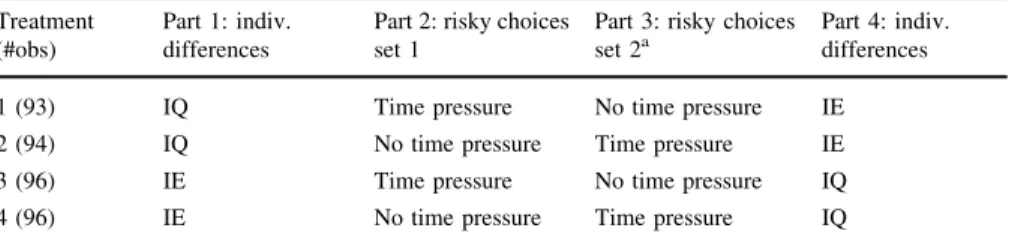
More specifically, for each participant we observe (a) risky choices in the absence of time pressure; (b) risky choices in the presence of time pressure; (c) a measure of cognitive ability (‘‘IQ’’); and (d) a measure of intellectual efficiency (‘‘IE’’). We discuss the different tasks and measures in detail below. The general structure of the experiment carefully counterbalances the order of the different parts as shown in Table1. The setup allows us to test the hypotheses (1) that those who violate the time constraint under time pressure make substantially different choices in the absence of time pressure; and (2) that behavior under the adverse influence of time pressure is predicted by decision makers’ behavior in the absence of time pressure and their observable traits.
Each set of risky choices (Set 1 and Set 2) consisted of 24 binary choices (see Table9 in ‘‘Appendix’’ for a full description). Time pressure was imposed by setting time limits for each of two 12-item subsets of choices within each of these
two sets of risky choices. In particular, each set consisted of (a) one subset of 12 binary choices that compared pure loss lotteries with mixed lotteries of lower expected value (‘‘prominent gain’’); and (b) one subset of 12 binary choices that compared pure gain lotteries with mixed lotteries of higher expected value (‘‘prominent loss’’). A detailed description and motivation of these choice tasks is given in Sect.2.3.4An important feature of the time pressure implementation is that the time limit was imposed on the subset level, not on each choice item.5That is, participants could go through the items in each subset at their own pace and therefore had to organize the allocation of time to the different choices efficiently.
However, subjects were not allowed to go back and reconsider earlier choices. In contrast to situations where time pressure is imposed on individual items, varying time pressure at the subset level adds an additional layer of complexity: Decision makers have to simultaneously allocate their time budget to the respective items, while considering the decision problem in the face of time pressure. This allows us to identify time management abilities and strategies to cope with time pressure of those who violate the time limit, and those who do not.
To make time pressure and no time pressure conditions as similar as possible in the presentation of the instructions and the task design, the unconstrained task also involved a time limit. However, this limit was selected such that it would not provide a binding constraint for subjects, namely at 420 s in all subsets. The extent of the time constraint in the time pressure conditions was calibrated in pre-test sessions such that there would be significant time pressure, while not making it impossible for the subjects to perform the decision task. In particular, under time pressure, the time limits were set at 120 s for the set with the prominent gains and at 80 s for the set with the prominent losses. In both cases, this value implied a 20%
Table 1 Treatment design Treatment
(#obs)
Part 1: indiv.
differences
Part 2: risky choices set 1
Part 3: risky choices set 2a
Part 4: indiv.
differences
1 (93) IQ Time pressure No time pressure IE
2 (94) IQ No time pressure Time pressure IE
3 (96) IE Time pressure No time pressure IQ
4 (96) IE No time pressure Time pressure IQ
IQ, measurement of cognitive ability; IE, measurement of intellectual efficiency; a, a set of pure gain choices was added after Set 2 to give subjects the possibility to earn back potential losses in sets 1 and 2 (see Sect.2.3). Note that the IQ and IE tasks allowed subjects to move back and forth across items while this was not possible in the risky choice tasks
4 Because losses were possible in the lottery choices, we included another set of lottery choices after the main task (Set 2/Part 3) that gave subjects the possibility to earn back any losses from sets 1 or 2. See Sect.2.3for details.
5 Both forms of time pressure are commonly observed in real-life and therefore important to study.
Gabaix et al. (2006) offer a good analogy of these two forms of time pressure in a context of a shopper at Walmart: time pressure imposed on individual items is analogue to buying a TV while considering its many attributes; time pressure imposed on set levels is similar to a situation where the shopper wants to buy other products (each with different attributes) within her time budget.
reduction of the median decision times in the absence of constraints that we observed in six pilot sessions (details about the pre-test sessions are given in the Web Appendix6).
2.1 Cognitive ability and intellectual efficiency
We employed Raven’s advanced progressive matrices (APM) test to measure cognitive ability(‘‘IQ’’) andintellectual efficiency(‘‘IE’’). Cognitive ability assesses a subject’s cognitive reasoning power, i.e. the extent to which complex information can be processed. Intellectual efficiency measures cognitive reasoning speed, i.e.
how fast incoming information can be processed (Raven et al. 1998). We hypothesized that IQ positively predicts decision quality, whereas lower IE predicts increases in the likelihood to violate the time constraint.
Cognitive ability constitutes a non-verbal estimate of fluid intelligence, the ability to reason and solve novel problems. Individuals with high fluid ability are thought to be able to better cope with time pressure, because they typically possess larger working memory (Shelton et al. 2010). In addition, De Paola and Gioia (2016) report that cognitive ability has a positive impact on performance under time pressure. Intellectual efficiency in turn imposes exogenous time pressure on the problem, such that we expect cognitive ability to be positively related to decision quality (defined in Sect.3), but intellectual efficiency to be predictive for the ability to complete all necessary decisions when time is scarce.
Raven’s advanced progressive matrices are aimed at subjects in the high cognitive ability ranges such as university students. In each item, subjects were presented with a 3-by-3 matrix of abstract symbols, with the symbol in the lower right corner missing. They were asked to choose, among eight possible alternatives, the one that completed the pattern in the matrix. We communicated to subjects that the items in the task were arranged in ascending order of difficulty and that they could go back and forth within the (possibly non-binding) time limit to revise their answers. An example can be seen in Fig.1, where the correct answer is option 3.
Instead of running the full 48-item test, a short-form7 containing 12 selected items from the APM test was administered to obtain a measure of IQ, as it has been argued that conducting the full APM does not add much predictive power (the correlation between the two formats isq= 0.88, see Bors and Stokes1998). As we are interested in the cognitive capacities of subjects, we allowed subjects to answer all twelve items at their own pace. To keep instructions as close as possible to our measure of intellectual efficiency (details below), we implemented a non-binding time constraint of 25 min, which was again calibrated in pre-tests.
6 The web appendix, data, and replication files will be made available athttps://heidata.uni-heidelberg.
de/dataverse/awiexeco.
7 The short form of the APM test we used here was introduced by Bors and Stokes (1998), consisting of items 3, 10, 12, 15, 16, 18, 21, 22, 28, 30, 31, and 34 of the APM (Set II). It is more difficult, and therefore suits university students better, than the other short version proposed earlier by Arthur and Day (1994).
We used the remaining 34 items8 from the APM to construct a measure of intellectual efficiency, i.e. the speed of cognitive reasoning, following Raven et al.
(1998, Section 4, APM15ff.) and Yates (1966). By imposing a severe time limit on subjects (13 min to solve all 34 items), we measure how fast and how efficiently they can process information. They could again reconsider earlier choices at any time. The timing constraint proved to be binding in pre-tests: no participant was able to finish all questions within the time limit.
Based on the tasks, we define our measures IQ and IE as the number of correct items in the cognitive ability and the intellectual efficiency tasks, respectively.
There was no additional reduction of the score for wrong answers or missing items.
Note that, as shown in Table1, the IQ and IE tasks were counterbalanced separately for each ordering of the time pressure tasks. The IQ and IE tasks were incentivized such that (1) a higher score yielded a higher chance to win a monetary prize, and (2) subjects could never identify their number of correct answers exactly. We provide more details on the rationale and the procedure in ‘‘Incentivization of cognitive ability tasks’’ in ‘‘Appendix’’.
2.2 Personality measures
At the end of the experiment, we elicited several personality measures that have often been linked to decision making (e.g., Nadkarni and Herrmann2010), and are potentially relevant to the ability of coping with time pressure. The generalized self- efficacy scale (Schwarzer and Jerusalem 1995) is a ten-item questionnaire which aims at measuring the ‘‘belief in one’s competence to tackle novel tasks and to cope
Fig. 1 A sample screen from Raven’s APM
8 We used the first two items in Set I of the APM test as instructional items, leaving 34 items for our intellectual efficiency measure. The items’ increasing difficulty was taken into account by preserving the items’ ordering.
with adversity in a broad range of stressful or challenging encounters’’ (Luszczyn- ska et al.2005, p. 80). Time pressure is thus a natural environment in which self- efficacy may have an effect on decision-making quality. In particular, in line with previous research showing a positive correlation between measures of self-efficacy and good financial planning behavior (Kuhnen and Melzer2014), we hypothesized that higher level of self-efficacy may be associated with better decision quality under time pressure. Rotter’s (1966) Locus of Control questionnaire is a 28-item survey that assesses the extent to which individuals believe that they have control over events that affect them in their lives. Whenever individuals feel to be in control, they might be less likely to perceive stress (e.g. generated by time pressure) as a threat (Chan1977). It has been shown that internally-oriented individuals are more likely to appraise stressful situations as a controllable challenge and focus on coping with stress, while externally-oriented individuals are more likely to be threatened by stressors (Bernardi1997; Folkman1984; Parkes1984). We therefore hypothesized that stronger internal orientation mitigates the effects of time pressure on decision making. A Big Five Ten Item questionnaire, measuring the Big Five personality characteristics with ten questions was also administered (see Gosling et al. (2003) for a comparison between this inventory and a widely used 44-item inventory). Here we predicted that traits such as neuroticism could become a burden under time pressure, as previous research has shown that this trait is positively associated with task avoidance (Matthews and Campbell1998), and Byrne et al.
(2015) have found that neuroticism is negatively correlated with performance in tasks with social and time pressure. Finally, we elicited general demographics and background data.
2.3 Risk preference measures
Our main task involved binary risky choices. We build on the design in Kocher et al.
(2013), who analyzed risky decisions under time pressure. That study found strong time pressure effects for lottery choices involving mixed gambles, i.e., including both gains and losses. In particular, under time pressure, decision makers seem to be prone to prefer mixed gambles over pure loss gambles with higher expected value (thus being drawn by the prominent gain in the mixed gambles); similarly, decision makers seem to prefer pure gain gambles over mixed gambles with a higher expected value (thus being repelled by the prominent loss in the mixed gamble).
Both Saqib and Chan (2015) and Conte et al. (2016) find similar prominence effects under time pressure. Because we want to study the role of selection effects under time pressure, we deliberately employed this particular structure of lottery choices, expecting to induce robust time pressure effects with the design. As described before, we presented subjects with two sets of choices, one set being time- constrained, and the other de facto unconstrained. Each set consisted of a subset of 12 choices of the prominent-gain format, and 12 choices of the prominent-loss format. The order of the two subsets was fixed, each subject first worked on the subset in the prominent-gain format, before moving on to the prominent-loss format.
The two subsets were separately time-constrained as described above. Within each subset, subjects had to proceed through the choice problems in a given order (fixed
over all subjects and conditions) and could not go back to revise previous choices. A list of all choices is given in ‘‘List of binary risky choices’’ in ‘‘Appendix’’. A screenshot of the presentation of the choices is given in ‘‘Graphical presentation of risky choices’’ in ‘‘Appendix’’.
Subjects made as many choices as possible within the time constraint. At the end of the experiment, one choice was selected randomly from all the potential choice problems in Set 1 and Set 2, and payoffs depended on the decision made, i.e. the lottery chosen, in this choice problem (this procedure prevented wealth or house money effects, which we considered relevant in the context of risky choice). If a subject violated the time constraint and thus failed to answer some of the questions, she would receive the lowest possible outcome (i.e., the highest possible loss) if one of the unanswered decision problems was selected for payment. This severe form of punishment encouraged subjects to always make a decision, and it is a common feature of many real-life decision environments with time pressure (e.g. air traffic control, emergency room doctors).9 For example, if the selected choice problem involved a choice between the lottery (15%:-€15, 85%:-€11) and (15%:€12, 85%:-€17) (see S1/G11 in Table9in ‘‘Appendix’’), the earnings for a person who did not submit a decision was-€17.
Because the risky choices of sets 1 and 2 involved potential losses, we needed to endow the participants with sufficient funds to cover any losses they might incur in parts 2 and 3 of the experiment. Therefore, an additional task was added after Set 2 that involved six risky choices between lotteries in which the lowest possible gain amounted to€20. By adding the endowment task after all Part 2 and Part 3 choices had been made, and by endowing with the help of risky choices, we prevented subjects from integrating the endowment easily with the loss outcomes in the choices in earlier parts. This method was adapted from Kocher et al. (2013). We did not impose a time limit on the endowment task. At the end of the experiment, one of the six choices was randomly selected for payment, and earnings were added to earnings from the lottery selected from sets 1 and 2. When working on Set 1 and Set 2, subjects were not aware how the subsequent task would look like; they only knew that other parts were to follow and that they would not incur overall net losses from the experiment. In the analyses below, we always report performance based on behavior in sets 1 and 2, thus not incorporating the endowment task.
2.4 Laboratory details
The experiment was programmed using z-Tree (Fischbacher2007) and recruitment was done with the help of ORSEE (Greiner2015). We conducted 16 experimental sessions at the MELESSA laboratory at the University of Munich in July and September 2014. In total, 379 subjects took part in the experiment, up to 24 in each
9 We intended to study an environment in which failing to meet the time constraint has clear and severe consequences. In particular, we wanted to implement a trade-off between making more thoughtful decisions and answering all decision problems. We did not want to add risky decision considerations to this trade-off by, for example, paying some metric like the expected value or selecting one option randomly. We observe that in most real world settings agents do not receive a randomly selected option, or an average payment, if they fail to choose in time.
session. 60% of the subjects were female with an average age of 24 years. They were mostly undergraduate and graduate students from the diverse set of programs that the university offers.10Payoffs were determined by randomly selecting one of the four parts for payment, with payment details then depending on the procedures described in the previous subsections. A typical session lasted for about 75 min, and subjects earned on average about€16.63 (approximately $21.32 at that time). In addition, we ran several pilot studies in Tilburg and Munich to calibrate the appropriate timing constraints. Information on the pilots, as well as the experimental instructions, can be found in the Web Appendix.
3 Time pressure and risky decisions: manipulation check
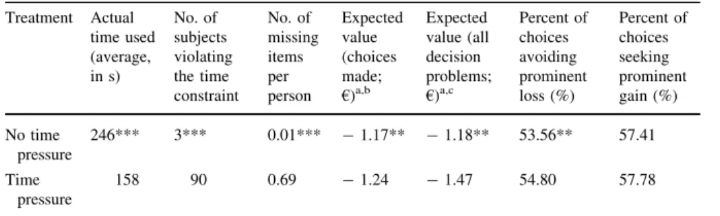
We first consider whether the time pressure manipulation for the risky decisions was effective in terms of time-use, in terms of the number of participants violating the time constraint, and in terms of the number of unanswered decision items. Table2 shows the results using the within-subject comparison.
Clearly, subjects made substantially faster decisions under time pressure, were more likely to violate the time constraint, and had more missing items. The manipulation of time pressure was successful in providing a highly adverse decision environment.
We next consider the effect of time pressure on risky decisions. The last four columns in Table2show, for time-unconstrained and for time-constrained choices, the average expected payoff that is implied by the choices the subject actually made, the average expected payoff that is implied by all choice problems including
Table 2 Time pressure manipulation for risky decisions Treatment Actual
time used (average, in s)
No. of subjects violating the time constraint
No. of missing items per person
Expected value (choices made;
€)a,b
Expected value (all decision problems;
€)a,c
Percent of choices avoiding prominent loss (%)
Percent of choices seeking prominent gain (%) No time
pressure
246*** 3*** 0.01*** -1.17** -1.18** 53.56** 57.41
Time pressure
158 90 0.69 -1.24 -1.47 54.80 57.78
Decision times reported show the sum of time used for the two subsets, S1 and S2. Total time constraint was 200 s under time pressure, and 840 s in the absence of time pressure
aAverages reported
bNumbers reflect the expected value implied by choices actually made
cNumbers reflect the expected value implied by all choice problems, including missing items
*, **, ***Significance of difference from time pressure condition at the 10, 5, and 1% level, Wilcoxon signed-rank test
1015% majored in economics, 16% in business administration, while 10% were enrolled in other social sciences programs. Furthermore, 4% were psychologists, 10% majored in the humanities, 5% in law, 21%
in the natural sciences or technology and the remaining rest 19% came from other fields.
missing items (which count as the highest loss),11 the percentage of choices that avoid a prominent loss, and the percentage of choices that seek a prominent gain.
The latter two percentages are conditional on the items that a person has answered.
We observe that overall, time pressure significantly reduces decision quality.12 The expected value (EV) implied by choices actually made is lower under time pressure. Additionally, missing items lead to losses and further reduce payoffs under time pressure. Under time pressure, participants make more choices that avoid a prominent loss (54.80%) than in the absence of time pressure (53.56%), at a loss of expected value (p\0.05). That is, choices are more heuristic under time pressure, being affected by salient attractive aspects of the lottery and sacrificing expected payoff. We observe that, despite the fact that the time constraint is imposed on the set level rather than the individual task level as in Kocher et al. (2013), our findings replicate the effects reported in their study.
Participants realize a lower expected value under time pressure. In the subsequent analyses, we consider expected value as a measure of decision quality. This interpretation is supported by the direct (inverse) link of expected value to heuristic choices (loss avoiding and gain seeking). Expected payoff is also a criterion that is applied in many professional settings outside the laboratory to assess decision success. However, participants may not necessarily aim to maximize expected value in the experiment. In the Web Appendix, we therefore present the main results also under the alternative assumption that participants’ decisions may reflect cumulative prospect theory preferences. In Sect.5.2, we report results taking the stability of the decision process (based on a fitted decision model) across settings as an alternative quality criterion.
4 Results: identifying selection
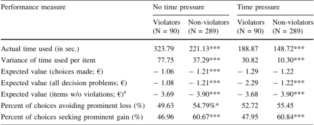
We first approach the question whether selection is relevant under time pressure. To this end, we compare those decision makers who violate the time constraint under time pressure (N = 90) to those who do not (N = 289). A violator is defined as a decision maker who ran out of time before making all 12 choices, in at least one of the two subsets of risky decisions in her time-constrained part.13Clearly, these two groups will thus differ under time pressure. However, the within-person design also allows us to study whether these groups differ when they arenottime-constrained.14
11As a benchmark for the subsequent analyses we observe that the highest realizable expected value was
€-0.39, and the lowest was€-2.28, if all choices were actually answered. Not answering any item would yield an expected payoff of€-11.23.
12Results are even more pronounced if we only consider data in Set 1 using between-subjects comparison. Set 2 behavior might be influenced by experience. We discuss possible learning effects in the Web Appendix, section B.5.
13We do not wish to invoke normative statements with respect to violating rules by choosing the term violator.
14In Sects.4and5, we report the average treatment effects of time pressure, pooling all decisions in Set 1 and Set 2 irrespective of order. Web Appendix B.5 provides additional analyses, reporting results based on either Set 1 or Set 2 data. Results do not differ qualitatively across the two sets. In Web Appendix B.4,
Table3 shows results of the comparison between the two groups for various measures. The left panel shows behavior in the absence of time pressure. Subjects who violate the time constraint differ substantially from those who do not violate the constraint in the way they approach the risky decision task. In terms of decision processes, violators use more time and distribute their time less evenly across choices. Moreover, violators are less affected by salient loss or gain features of the lotteries. They consequently perform significantly better on average in terms of the implied expected value of their choices than non-violators, when not exposed to time pressure. In the right panel of Table3, we compare the two groups in the presence of time pressure. Also, under a time constraint, violators use more time and have a higher variance of time used across choice problems. They perform significantly worse on the full set of choices. This effect is driven by the relatively strong punishment for not answering a choice problem, which they seem not to take sufficiently into consideration in their strategy. Moreover, under time pressure, violators do not perform better than non-violators on the choices they actually made.
However, violators do not perform significantly worse than non-violators on these items either.
Table3 also shows the expected value over the set of choices for which no subject violated the time constraint (row five).15This includes the first seven choices in the prominent gain sets and the first three choices in the prominent loss sets.
Table 3 Differences between time-constraint violators and non-violators
Performance measure No time pressure Time pressure
Violators (N = 90)
Non-violators (N = 289)
Violators (N = 90)
Non-violators (N = 289)
Actual time used (in sec.) 323.79 221.13*** 188.87 148.72***
Variance of time used per item 77.75 37.29*** 30.82 10.30***
Expected value (choices made;€) -1.06 -1.21*** -1.29 -1.22 Expected value (all decision problems;€) -1.08 -1.21*** -2.29 -1.22***
Expected value (items w/o violations;€)a -3.69 -3.90*** -3.68 -3.90***
Percent of choices avoiding prominent loss (%) 49.63 54.79%* 52.72 55.45 Percent of choices seeking prominent gain (%) 46.96 60.67*** 47.95 60.84***
Violator status for each subject is assigned if at least one item in at least one time-constrained subset was not answered
aExpected value calculated on the basis of those items in the prominent gain and prominent loss subsets thatallsubjects were able to answer under time pressure
*, **, ***at the entries for non-violators indicate that these values differ from those for violators, at the 10, 5, and 1% significance level, two-sided Mann–Whitney tests
Footnote 14 continued
we also report on a continuous measure number of items missed rather than the violator indicator. Results replicate results presented in the main text.
15For this row, we removed one subject, a violator, from the analysis in this table, as she is the only participant violating the time constraint already at the fourth item for the subset of prominent gain lotteries, while others violate only after the seventh item. The results remain the same if we include all subjects but we lose a substantial amount of information for the subset of prominent gain lotteries.
Apparently, on this subset of early choices, the violators perform much better than the non-violators do, and this holds true in both the time pressure and the no-time pressure condition. Moreover, comparing this performance measure across time pressure conditions, we observe that the expected payoffs do not differ for either group of decision makers (for both groups,p[0.7, Wilcoxon signed-rank test).
Thus, under time pressure, initially the violators can fully implement the same decision strategy as in the absence of time pressure. However, in later decision items when less time is available, they lose out, harming their overall performance for the choices they actually make (shown in row three in Table3) and even more so for the full set of choices (shown in row four in Table3).
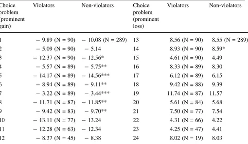
This dynamic pattern of performance is shown in more detail in Table4. The table shows for each item, in the order of appearance, the implied expected value of the choices made by violators and non-violators under time pressure. In the set of prominent gains (items 1–12), violators perform better early on. In the set of prominent losses (item 13–24), the effect is less pronounced, but points in the same direction. As they move on with the task, violators do not make better decisions than the non-violators anymore, possibly because time becomes scarce. This is especially true in the set with prominent gains. Additionally, violators at some point violate the time constraint (shown by the decrease in sample sizes indicated for each choice item), leading to significant losses in expected value over all decision problems. We also observe that violation of the time constraint for prominent-loss choices leads to
Table 4 Differences between time-constraint violators and non-violators across choice items under time pressure (expected value of choices made)
Choice problem (prominent gain)
Violators Non-violators Choice
problem (prominent loss)
Violators Non-violators
1 -9.89 (N = 90) -10.08 (N = 289) 13 8.56 (N = 90) 8.55 (N = 289)
2 -5.09 (N = 90) -5.14 14 8.93 (N = 90) 8.59*
3 -12.37 (N = 90) -12.56* 15 4.61 (N = 90) 4.49
4 -5.57 (N = 89) -5.75** 16 8.33 (N = 89) 8.30
5 -14.17 (N = 89) -14.56*** 17 6.12 (N = 89) 6.15
6 -8.94 (N = 89) -9.11** 18 9.42 (N = 88) 9.39
7 -3.22 (N = 89) -3.44*** 19 11.74 (N = 87) 11.57
8 -11.71 (N = 87) -11.85** 20 5.61 (N = 84) 5.68
9 -9.42 (N = 83) -9.70** 21 7.50 (N = 77) 7.54
10 -13.11 (N = 77) -13.24 22 4.31 (N = 66) 4.22
11 -12.28 (N = 63) -12.34 23 4.25 (N = 47) 4.41
12 -8.37 (N = 45) -8.38 24 8.02 (N = 19) 8.03
Entries are expected values (€) of choices made; averages over participants in the subgroup
*, **, ***at the entries for non-violators indicate that these values differ from those for violators, at the 10, 5, and 1% significance level, Mann–Whitney tests. Number of observations in parentheses (constant for non-violators)
an additional loss of expected payoffs for the set of choices made. This is caused by the fact that lotteries in this subset had positive expected payoffs, and thus a participant’s average expected payoff over choices made is harmed by simply reducing the number of prominent-loss choices that are completed. This effect leads to the negative effect on expected value for choices actually made under time pressure, shown in row three of Table3.
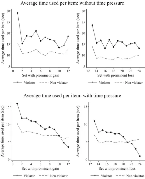
Figure2 further illustrates different time-use strategies employed by violators and non-violators by plotting the average decision time they spend on each item.
The strategy violators employed resembles the notion of ‘‘maximizer’’, first discussed by Simon (1955,1956) and formalized by Schwartz et al. (2002), in which decision makers only settle for the best option. On the other hand, non-violators seem to use a strategy in line with the notion of ‘‘satisficers,’’ who settle for an option that seems good enough. In the absence of time pressure (upper panel), violators clearly spend more time on each item than non-violators, and use a substantial amount of time for some items that might be perceived as more difficult by them, leading to higher variance in terms of the average time-used per item. In the Web Appendix (Section B3) we provide additional analyses. Using panel regressions to explain the time used on each item in the absence of a time constraint, we find that violators on average use 6 s more on each item and that they are much more sensitive to the difficulty of the expected value calculation than non-violators.
These results further support the notion that violators seem to behave as
‘‘maximizers’’. Under time pressure (lower panel in Fig.2), violators initially use much time and then almost monotonically reduce their time used per item as they progress through the task.16 Compared to the non-violators who remain relatively stable in their time use per item as they proceed through the task, violators thus initially use more time, and later have even less time than the (on average) non- violators take for the last few items. That is, given the significant punishment for violation of the time constraint, violators exhibit poor time management.
An important question regarding the external validity of experimental observa- tions of choice behavior concerns the correlation between time-constrained and unconstrained behavior at the individual level. We observe that behavior and outcomes are positively correlated across environments. Yet, correlations are larger for non-violators than for violators.17 While non-violators seem to be able to implement similar decision strategies both in the absence and in the presence of time pressure, violators are less able to sustain the same strategy in the different decision environments, especially for the last few items when they run out of time.
16All items that a person cannot answer because time ran out are counted as zero time used. This is consistent with the person having indeed used zero seconds to make the decision. Note that the non-zero time use for later items in each subset by each group of violators is caused by the definition of violator based on a violation inat leastone of the two subsets. Thus, not all violators run out of time in the prominent gain subset (prominent loss subset)
17Results can be found in the Web Appendix, Table W11.
To sum up, we document substantial selection effects under time pressure: those participants who cannot cope with the time constraint have very different time-use and decision strategies in the absence of time pressure. They make better decisions when sufficient time is available (i.e., under no-time pressure conditions) than those subjects who are not violating time-constraints under time pressure. However, under time pressure they are not able to sustain these strategies anymore and therefore lose out against the non-violators in terms of performance.
5 10 15 20 25 30
Average time used per item (sec)
0 2 4 6 8 10 12
Set with prominent gain Violator Non-violator
5 10 15 20 25 30
Average time used per item (sec)
12 14 16 18 20 22 24
Set with prominent loss Violator Non-violator
Average time used per item: without time pressure
0 5 10 15
Average time used per item (sec)
0 2 4 6 8 10 12
Set with prominent gain Violator Non-violator
0 5 10 15
Average time used per item (sec)
12 14 16 18 20 22 24
Set with prominent loss Violator Non-violator
Average time used per item: with time pressure
Fig. 2 Time use of violators and non-violators
5 Results: time pressure resistance—predicting who can better cope with time pressure
5.1 The effect of observable traits: non-parametric analyses
Having observed that there are systematic differences in behavior between those who can and those who cannot cope with time pressure well, we now investigate whether there are observable traits or characteristics that allow predicting time pressure resistance in risky decision making. We observe significant lower intellectual efficiency and self-efficacy among violators (IE: 22.47 vs. 23.27 for non-violators, SE: 28.36 vs. 29.80 for non-violators, Mann–Whitney tests, both p\0.05). While not significant on conventional levels, there exist suggestive differences in gender (29.31% male vs. 40.46% male for non-violators, Mann–
Whitney test,p = 0.14).18For none of the Big Five items were there any differences between violators and non-violators. Moreover, in the previous section we have already shown the pronounced differences in time use strategies between violators and non-violators. In the following we therefore study the differences between low and high IQ, low and high IE, low and high self-efficacy, and small and large amounts of time used/variance of time used (in the absence of time pressure).
Importantly, these differences are observed forallsubjects, irrespective of whether they violate the deadline under time pressure or not. That is, we can also make use of variation in performance within the groups of violators and non-violators. Below we will use these measures also jointly in a multivariate analysis as predictors of decision performance under time pressure.
5.1.1 Cognitive ability and intellectual efficiency
We consider the role of IQ and IE on risky behavior, in time-constrained and unconstrained settings. Despite being positively correlated (0.5760, p\0.01, Spearman rank correlation),19the correlation between IQ and IE is far from perfect, suggesting that the two measures capture separate traits. Since we are interested in outcomes and in selection effects, we report effects on the implied expected value from the choices made and from all choice problems, the percentage of time- constraint violators, the number of missing items per subject, and the incidence of avoiding prominent losses and seeking prominent gains. Columns 1–4 of Table5 report the results for IQ and IE.
To allow for direct group comparisons, we split the sample at the median values of IQ and IE.20As shown in the table, in the absence of time pressure, low IQ and
18We analyze gender effects in Web Appendix B.1.
19A related measure of intellectual efficiency was introduced by Gough (1957), as part of the California Psychological Inventory. Similar to our findings, their measure of IE also correlated with several measures of cognitive ability: It correlated 0.58 with scores on the Terman Concept Mastery Intelligence Test, 0.50 with scores on the Kuhlman-Anderson Intelligence Test, 0.44 with scores on the Miller Analogies Test.
20The median IQ is 10. We split the sample such that IQ\10 defines the ‘‘low’’ group. The median for IE is 23. We split the sample such that IE\23 defines ‘‘low’’ group. In Web Appendix B.4 we consider continuous measures as robustness checks replicating the results qualitatively.
Table5Effectsofpersonaltraitmeasuresandperformance PerformancemeasureNotimepressure (840s=420?420)Timepressure (200s=120?80)Notimepressure (840s=420?420)Timepressure (200s=120?80)Notimepressure (840s=420?420)Timepressure (200s=120?80) IQHighIQLowIQHighIQLowIEHighIELowIEHighIELowSEHighSELowSEHighSELow Actualtimeused(ins)257.72228.62159.29156.82250.96237.38157.44159.48357.02230.75158.38158.10 Expectedvalue(choicesmade; €)-1.10-1.27***-1.14-1.37***-1.13-1.24***-1.19-1.30-1.17-1.18-1.28-1.18 Expectedvalue(alldecision problems;€)-1.11-1.27***-1.41-1.56**-1.13-1.24***-1.42-1.54-1.17-1.18-1.47-1.48 Percenttime-constraint violators(%)1.36024.0923.271.32022.4725.660.471.2020.6627.71 Numberofmissingitemsper person0.0100.700.680.0100.630.780.0050.0120.620.78 Percentofchoicesavoiding prominentloss(%)49.1759.64***50.3361.00***49.7159.32***51.9259.11**52.8254.5254.5855.08 Percentofchoicesseeking prominentgain(%)52.1764.68***54.5662.24***54.5661.68**57.5758.0957.5257.2857.9957.50 *,**,***attheentriesforIQLow,IELow,andSELowindicatethatthesevaluesdifferfromthoseforIQHigh,IEHigh,SEHigh,atthe10,5,and1%significancelevel,two-sided Mann–Whitneytests.ThemedianIQscoreis10.ThemedianIEscoreis23.ThemedianSEscoreis29
low IE subjects perform worse in terms of expected payoffs, and they are affected more strongly by salient features of the lottery than high IQ and IE groups. These results are consistent with previous findings in the literature (e.g., Dohmen et al.
2010). The table also suggests that the amount of time used by high IQ/IE subjects and relatively low IQ/IE subjects is similar, in both conditions.21Interestingly, the table shows show that IQ is correlated with decision quality under time pressure, while IE is not. The fact that IQ effects remain significant under time pressure suggests that the absence of an effect for IE is not simply due to a larger noise under time pressure. Note that we consider univariate correlations, and IE and IQ may be differently affected by other variables that are related with behavior under time pressure (e.g., gender), which will be controlled for in the multivariate analyses below.
5.1.2 Self-efficacy
Columns 5 and 6 of Table5 show results for self-efficacy. Although self-efficacy directly measures individuals’ ability to cope with hassles, similar to IE, there is no raw correlation with behavior and performance under time pressure and without time pressure.
5.1.3 Time-use strategies
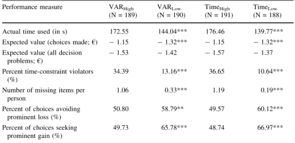
As seen before, time-use strategies differ strongly across subjects and correlate with violator status. Measuring the total time use and the variance across choice items in the conditions with no time pressure for all subjects, we confirm the importance of the measures. Table6 shows strong effects on violator status and missing items:
those who make more careful decisions (higher time use and variance) are more likely to violate the time constraint and miss out on answering items.22 However, these careful decision makers do not perform worse on average than the less careful ones. If they manage to meet the time constraint, they realize a higher performance.
Moreover, more careful decision makers are less prone to salience effects and obtain higher expected payoffs on the choices they make.
5.2 Fitting a cumulative prospect theory decision model
Tables5and6 demonstrate that observable characteristics are strongly associated with risky behavior in the presence and absence of time pressure. A natural question is whether we can link observable traits to a person’s ability to maintain her decision processes under a tight time constraint. To answer this question, we make use of the within-subject design to estimate a simplified cumulative prospect theory model (CPT, Tversky and Kahneman 1992) for each participant on the basis of her 24 time-unconstrained choices, assuming that these unconstrained reflect her
21This finding might derive from high-ability participants more carefully considering the decision, and low-ability participants taking more time to understand the problem.
22Similar to the previous analysis, we provide continuous measures in Web Appendix section B.4.
preferences. We then assess how successfully these preferences are implemented under time pressure. Predictive success is then related to observable characteristics.
Detailed methods and results are in Web Appendix A. Here we concisely state the main results. The fitted CPT model has good predictive power.23 The overall average success rate of predicting choices made under time pressure using time- unconstrained fitted parameters is above 65%, which is significantly better than a random prediction (p\0.01, Wilcoxon signed-rank tests). We find strong links between observables and predictive success. For decision makers with higher measures of IE, higher measures of self-efficacy, and less time-use in the absence of time pressure, the fitted model predicts behavior under time pressure more successfully than for those with lower measures in the respective comparison categories. For IQ and variance in decision times, we find insignificant results. Thus, there is clear evidence that observables relate to a person’s time pressure resistance.
Importantly, in contrast to an evaluation based on expected payoffs, the current approach presumes no normative measure of success apart from stability of preferences between the two environments; each person is evaluated on the basis of her own choice behavior in the absence of time pressure, possibly showing loss aversion and/or probability weighting.
Table 6 Effects of variance of time used per item and total time used (in the absence of time pressure) on outcomes under time pressure
Performance measure VARHigh
(N = 189)
VARLow
(N = 190)
TimeHigh
(N = 191)
TimeLow
(N = 188)
Actual time used (in s) 172.55 144.04*** 176.46 139.77***
Expected value (choices made;€) -1.15 -1.32*** -1.15 -1.32***
Expected value (all decision problems;€)
-1.53 -1.42 -1.57 -1.37 Percent time-constraint violators
(%)
34.39 13.16*** 36.65 10.64***
Number of missing items per person
1.06 0.33*** 1.19 0.19***
Percent of choices avoiding prominent loss (%)
50.80 58.79** 49.57 60.12***
Percent of choices seeking prominent gain (%)
49.73 65.78*** 48.74 66.97***
*, **, ***at the entries for VARLowand TimeLowindicate that these values differ from those for VARHigh
and TimeHigh, at the 10, 5, and 1% significance level, two-sided Mann–Whitney tests. The median variance of time used per item under no time constraint is 12.74. We split the sample such that VAR\12.74 is the low variance group; and time\201 s is the low time (faster) group. Total time was 200 s (in time pressure conditions)
23It turns out that violators are significantly more loss averse (p\0.001) and have a lower probability weighting parameter (p\0.06). This suggests another pathway through which violators may differ systematically from non-violators.
5.3 Multivariate analyses
We next provide multivariate analyses for our main dependent variables of interest.
We study the partial correlations of IE, IQ, self-efficacy, gender, as well as our two time-use measures with the expected payoffs for the choices made (columns 1 and 2 in Table7) and with the expected value over all choices (columns 3 and 4 in Table7), under time pressure. That is, we aim to identify whether using a set of observables allows us to predict outcomes under time pressure. In addition, we also conduct multivariate analyses for predictive success of the fitted CPT model under time pressure, both for choices made (column 5 in Table7) and for all decision problems (column 6 in Table7).
The results confirm our earlier findings but show overall modest explanatory power of background variables for variations in expected payoff and predictive power of individual decision models under time pressure. IQ and IE, which are positively correlated, are significant predictors of expected value and predictive success. As expected, IE seems more relevant for all choices (including missed items), while IQ is more relevant for choices made. F-tests suggest that IE and IQ jointly determine the decision quality, with higher ability participants making better choices (EV) and more consistent choice across time pressure settings. Total time used in the absence of time pressure predicts better decisions over choices made, but lower predictive success over all choices. We find no significant effect of gender.
Self-Efficacy has a significant effect only for predictive success over all choices made.
Overall, we can explain only a small amount of the variance in expected value and in predictive success of the fitted CPT model. Although IE, IQ and time used strategy under unconstrained conditions are helpful in predicting decisions, our results still emphasize the necessity of finding better instruments to predict the ability to perform under time pressure.
6 Discussion
We set out to study the role of selection in time-pressured decision environments, and how it is linked to observable characteristics of the decision maker, including those characteristics that can be made observable using survey and experimental techniques. Clearly, different decision styles play an important role. Those who can and those who cannot easily cope with the time constraint in risky decisions differ along various dimensions. People who violate time constraints, i.e. those with lower time pressure resistance, make more careful (more variance, more time used), and consequently more successful decisions (higher EV, less affected by salient outcomes) when unconstrained. They also initially perform better under time pressure. However, as they run out of time, they cannot implement their strategy anymore, leading to considerable losses. Consequently, their performance and behavior are also much less correlated between the time pressure and the no- pressure conditions than it is the case for non-violators. A fitted decision model on the basis of behavior in the absence of time pressure, is less predictive of their