Lifetime estimation and performance evaluation for offshore wind farms transmission cables

Lifetime estimation and performance evaluation for offshore wind farms transmission cables

Published in 15th IET international conference on AC and DC Power Transmission, Coventry

Feb 2019

Copyright:

Reproduction of this publication in whole or in part must include the customary bibliographic citation, including author attribution, report title, etc.

Cover photo: Copyright: Stiftung Offshore-Windenergie• Eon- Netz • Detlef Gehring • 2008

Published by: Baltic InteGrid Disclaimer:

The content of the report reflects the author’s/partner’s views and the EU Commission and the MA/JS are not liable for any use that may be made of the information contained therein. All images are copyrighted and property of their respective owners.

Lifetime estimation and performance evaluation for offshore wind farms transmission cables

Published in 15th IET international conference on AC and DC Power Transmission, Coventry

By Juan-Andrés Pérez-Rúa, Kaushik Das, Nicolaos A. Cutululis, Department of Wind Energy, Technical University of Denmark, Denmark

1

Lifetime estimation and performance evaluation for offshore wind farms transmission cables

Juan-Andrés Pérez-Rúa*, Kaushik Das*, Nicolaos A. Cutululis*

*Department of Wind Energy, Technical University of Denmark, Frederiksborgvej 399, 4000 Roskilde, Denmark. E-mail:

juru@dtu.dk Keywords: Offshore wind energy, transmission cables, dynamic temperature prediction, thermo-electrical stress, probabilistic lifetime estimation.

Abstract

A novel methodology for life estimation and performance evaluation of offshore wind farms high voltage AC export cables is presented. The method applies Dynamic Temperature Prediction (DTP) analysis using a Thermo-Electrical Equivalent model (TEE). Furthermore, it is suggested how the cable lifetime might be inferred based on the accumulated ageing effects. Afterwards, a sensitivity analysis of the seabed temperature variations is performed. Finally, a holistic procedure for calculating more accurately the electrical power losses of the cable is presented. Results show that an important increase of the total installed power, or cross-section reduction, can be achieved compared to traditional sizing methods.

1 Introduction

Offshore wind energy represents one of the fastest and most steadily growing renewable technologies. The penetration level has increased almost five times in the last seven years, reaching the impressive globally total installed power of nearly 19 GW [1]. The grid connection for Offshore Wind Farms (OWFs) contributes to around 15 % of the total system costs [2]. The export cable is one of the most important components in this concept, partly because of the increasingly longer distance from shore, and partly because of its direct impact on the overall availability [3].

Currently, the sizing of the offshore export cables is done according to the CIGRE and IEC standards [4]. However, such standards consider steady state conditions under rated operation, i.e., a continuous conductor temperature equal to 90 ℃ and nominal electric field. The limitation of the conductor temperature at this value is due to the close contact with the insulation material, which represents the most critical element in a cable.

In fact, in [5] is proved that other factors such as mechanical stress, and environmental stress, can be neglected thanks to the improvement of manufacturing techniques, and by the installation conditions of the cable itself (which is buried and protected by inner layers). Joints and terminals also deserve attention to maximize the lifetime of the export infrastructure.

Simultaneous electro-thermal stress represents the main ageing factor of the insulation, and consequently, of the whole cable.

These standards’ criterion may be intuitively too conservative considering that OWFs present a typical capacity factor of around 0.4-0.5. To cope with this issue, different concepts need to be combined in order to develop a methodology capable of estimating the lifetime of cables operating under real conditions, such as: time-varying cyclic power generation, thermal and electrical stress, thermal transients, capacity currents and failure probability.

This paper is divided in the following manner: The Section 2 describes the full model, then the TEE calibration is presented in the Section 3, and finally, it is reported the application of the Dynamic Temperature Prediction (DTP) model to a 245-kV cross-linked polyethylene (XLPE)-insulated cable, operating at realistic time-varying conditions. The potential cross-section reduction from the point of view of electro-thermal is pointed out. Conclusions extracted after this work close the article.

2 Model description

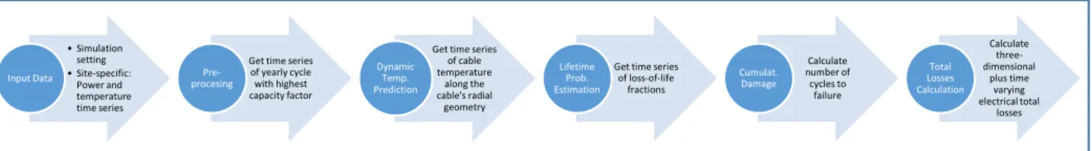
The scheme of the general proposed methodology is presented in the Figure 1. Input data is obtained after simulating offshore power generation, at a particular site, using the software described in [6].

Overall, this methodology is proposed aiming to develop a tool, which provides the first steps towards the offline dynamic loadability of transmission cables for offshore wind farm applications. In the next subsections, a descriptive explanation of each block will be presented. This paper focuses specially in the description, and analysis of the DTP model.

2.1 Pre-processing stage

In this stage is decided the period under which the cable is subject to operate. Different criteria might be defined in order to establish the basis cycle, one of them could be, for instance, the year with highest capacity factor, or that year with highest instantaneous conductor temperature. Studying on detail the best decision for selecting this period is out of scope in this paper, and future publications will deal with this matter.

2.2 Conductor dynamic temperature prediction

Reference [4] provides a set of equations that allow calculating the current to be transmitted in an infinite time period, in order to get a desired constant temperature, under given specific input conditions, such as buried depth, distance between phases, surrounding constant temperature, soil resistivity, etc.

Figure 1: Proposed general methodology.

However, for cases where the load current does not follow a constant profile, but rather a cyclic profile, the standard IEC-60853-2 defines mathematical expressions to correct a cable rating subject to these conditions, but the cycle is limited to some pre-defined discrete patterns, like pulse or triangular trains. On that account, dynamic loadability techniques calculate the current that can be carried for a limited period, without the physical limitations of any part of the cable being exceeded. Dynamic loadability requires the use of Dynamic Thermal Rating (DTR) in order to estimate the cable temperature either for real-time applications or for offline predictions given time series of forecasted load current (DTP). Nowadays, there are mainly three modelling principles for estimation of the cable temperature dynamically: finite elements (FEM), step response (SR) -used by CIGRÉ- and thermoelectric equivalent method (TEE). A comparison between those methods has been done in [7] and [8], where it is remarked that TEE provides results which are within an acceptable range of the FEM simulations (nearly 1℃) with a considerable computation time reduction. TEE models also have proved to exhibit a correct estimation of the temperature as compared to real measured data in experimental tests, with deviations of around 3℃ [9].

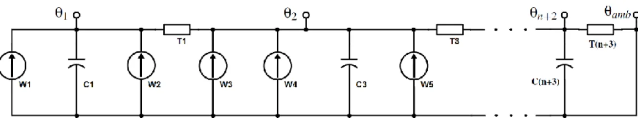
The TEE method is straightforward from an electrical engineering point of view. It basically consists in a direct translation of thermodynamic variables into electrical variables, i.e., considering the heat flow as electrical current and temperature as nodal voltages. Every layer of the cable is then represented with its thermal resistance 𝑇_𝑚 and its thermal capacitance 𝐶𝑚, along with the electrical losses; all together form the equivalent circuit presented in the Figure 2. The surrounding, which in the case of submarine cables is defined by the seabed where the cable is buried, can be also divided into multiple layers (𝑁), in order to obtain a more accurate DTP calculation, at cost of a higher computational time required. Equations for calculating the thermal parameters of the cable layers, and surroundings can be found in [8].

The mathematical expression of the system introduced in the Figure 2, under dynamic state applying Kirchhoff laws, is given in the Equation (1). In this equation the matrix 𝐴 is square and (𝑁 + 2)-dimensional, and its elements are dynamically defined by the total number of sublayers, 𝑁.

This expression consists of a system of ordinary differential

equations (ODE); 𝜃₁(𝑡) represents the time-varying conductor surface temperature, and 𝜃_𝑁+2(𝑡) correspondingly for the penultimate surrounding layer. It can be appreciated what was mentioned before: the system of equations, once solved, provide information of temperature along different points of radial distance from the cable's center. Additionally, it is inferred the fact that the conductor, screen and armature losses are dependent on the infeed power time series corresponding to the year selected in the pre-processing stage.

[ 𝜃_𝑛+2̇ (𝑡) 𝜃_𝑛+1̇ (𝑡)

⋮ 𝜃₃(𝑡)̇ 𝜃₂̇ (𝑡) 𝜃₁(𝑡)̇ ]

= 𝐴 [

𝜃_𝑛+2(𝑡) 𝜃_𝑛+1(𝑡)

⋮ 𝜃₃(𝑡) 𝜃₂(𝑡) 𝜃₁(𝑡) ]

+

[

𝜃_𝑎𝑚𝑏(𝑡) 𝑇(𝑛 + 3)𝐶(𝑛 + 3)

0

⋮ 0 𝑊2 + 𝑊4(𝑡) + 𝑊5(𝑡)

𝐶3 𝑊3 + 𝑊1(𝑡)

𝐶1 ]

(1)

Where the variables shown in the Figure 2 are:

• 𝑊1, 𝑊2, 𝑊3, 𝑊4, 𝑊5 = Conductor Joule losses (function of the input power), 50% of dielectric losses, 50% of dielectric losses, screen losses (function of the input power), and armature losses (function of the input power), respectively. All in (𝑊/𝑚).

• 𝐶1 = 𝐶𝑐+ 0.5𝐶𝑖. Where 𝐶𝑐 and 𝐶𝑖 are the conductor and insulation thermal capacitances, respectively. All in (𝐽/Km).

• 𝐶3 = 𝐶_𝑠+ 0.5𝐶_𝑖+ 𝐶_𝑎+ 𝐶_𝑗 . Where 𝐶_𝑠, 𝐶_𝑖, 𝐶_𝑎, and 𝐶_𝑗 are the screen, insulation, armature and jacket thermal capacitances, respectively. All in (𝐽/Km).

• 𝐶(𝑛 + 3)= Thermal capacitance of the surrounding sublayer 𝑛 in (𝐽/Km).

• 𝑇1, 𝑇3, 𝑇(𝑛 + 3) = Thermal resistance of the insulation, jacket and the surrounding sublayer 𝑛, respectively. All in (Km/W).

• 𝜃1, 𝜃2, 𝜃𝑛+2, 𝜃𝑎𝑚𝑏 = Instantaneous temperature at the surface of the conductor, insulation, surrounding sublayer 𝑛, and seabead, respectively.

All in (K).

The current along the cable is calculated with Equation (2), where 𝑉_𝑅(𝑧), 𝑉_𝑆, 𝛾, 𝑧, 𝑍_𝑐, 𝐼_𝑅(𝑧), and 𝐼_𝑠, are voltage vector at 𝑧 from the Offshore Substation (OSS), voltage vector at OSS, transmission coefficient, current vector at distance 𝑧 from the OSS, and current vector at OSS, respectively [10].

•Simulation setting

•Site-specific:

Power and temperature time series Input Data

Get time series of yearly cycle with highest capacity factor Pre-

procesing

Get time series of cable temperature

along the cable's radial

geometry Dynamic

Temp.

Prediction

Get time series of loss-of-life

fractions Lifetime

Prob.

Estimation

Calculate number of cycles to

failure Cumulat.

Damage

Calculate three- dimensional

plus time varying electrical total

losses Total Losses Calculation

3

Figure 2: Thermo-Electrical Equivalent (TEE) circuit model for a single-core high voltage submarine cable.

𝑉𝑅(𝑧) = 𝑉𝑠cosh(𝛾𝑧) − 𝐼𝑠𝑍𝑐sinh(𝛾𝑧) 𝐼_𝑅(𝑧) = 𝐼𝑠cosh(𝛾𝑧) −𝑉_𝑠

𝑍𝑐

sinh(𝛾𝑧) (2) Where 𝑉𝑠 is the nominal or maximum voltage level of the transmission system, and 𝐼𝑠= 𝑓(𝑉𝑠, 𝑃𝑠𝑒𝑟𝑖𝑒𝑠_𝑦). Therefore, 𝐼𝑅 can be calculated for a given distance 𝑧, and the inputs for Equation (1) are obtained: 𝑊1 = 𝑓(𝑅_𝑐(𝜃₁), 𝐼_𝑅(𝑧)), 𝑊4 = 𝑓(𝑅_𝑐(𝜃₁), 𝐼_𝑅(𝑧)), 𝑊5 = 𝑓(𝑅_𝑐(𝜃₁), 𝐼_𝑅(𝑧)). 𝑊2 and 𝑊3 are dependent only on the transmission voltage level.

The analysis must be carried out for the value of 𝑧 which brings the most critical thermal performance of the cable; in a AC system without series and parallel compensation, the most critical point is the onshore subestation due to the great capacitive currents typical in submarine cables.

2.3 Lifetime probabilistic estimation

There are several lifetime probabilistic models available in the literature, such as Zurkov, Crine, and Arrhenius-IPM, each within the probabilistic framework needed for associating time-to-failure to reliability. All these models present different analytical expressions and parameter values, however in general they all provide same indications regarding lifetime in function of time-varying electro- thermal stress. The Arrhenius-IPM model seems to be the most conservative over a wide operation range. By means of accelerated test experiments, the parameters of the Arrhenius-IPM model can be calculated accordingly, with subsequent updates considering new manufacturing processes and different cables [11].

2.4 Cumulative damage

One of the simplest models for quantifying cumulative damages for materials, is the one popularized by M.A.

Miner in 1945 [12]. See Equation (3), lifetime of a component is obtained when the sum of loss-of-life fractions is equal to one; this model makes use of stress- expected values, ignoring the probabilistic nature of the problem, and considering a linear life-stress relationship [13]. To overcome these limitations, in the framework of modern accelerated tests, and lifetime calculations, Miner’s law must be combined with proper failure-time probability density functions. Weibull distributions is usually the most appropriate for performing these studies.

∑𝑘 𝑊𝑖 𝑖=1

𝑊𝐹𝑎𝑖𝑙𝑢𝑟𝑒

= 1 (3)

2.5 Total losses calculation

The total losses calculation process allows a holistic estimation, taking into consideration the spatio-temporal variations of current along the cable [14]. The Dynamic Temperature Prediction explained in Section 2.2, includes the effects of conductor resistance variation in function of its temperature, which in turn changes with time and modifies the value of joule losses and other associated (screen and armature losses). Consequently, the total losses (𝑇𝐿) calculation is defined in the Equation (4).

𝑇𝐿 = ∫ ∫ 𝑅𝑐(𝑙, 𝑡) ∙ 𝐼(𝑙, 𝑘)²

𝑡 𝑙

≈ ∑ ∑ 𝑅𝑐(𝑙. 𝑘) ∙ 𝐼(𝑙, 𝑘)²

ℎ

𝑘=1 𝑙_𝐷𝑇

𝑙=1

(4)

In the Equation (4), 𝑙𝐷_𝑇, ℎ, 𝑅𝑐(𝑙, 𝑘), and 𝐼(𝑙, 𝑘) are the total number of sections that the cable is divided, total number of hours in a year, conductor resistance in ohms, and current in amperes, being the two last function of distance and time.

The higher 𝑙𝐷_𝑇 the more accurate the calculation but at the same time, more computational requirements; a proper balance between both parameters must be determined.

3 TEE model calibration

The value of the number of sublayers (𝑁) to divide the seabed is determined by means of a model calibration process, which consists in evaluating the computational time against the solution quality earned when 𝑁 is increased. To solve the system of equations, a non-stiff differential equations solver using medium order method is applied and performance indices are defined for quantifying the obtained solution quality. Let the Normalized Mean Absolute Error (𝑁𝑀𝐴𝐸_𝑁) [15], defined as (5), when using 𝑁 sublayers in total, and having as a reference the solution 𝑁_𝑚𝑎𝑥.

𝑁𝑀𝐴𝐸𝑁=1

ℎ∑ |𝜃1𝑘,𝑁− 𝜃1𝑘,𝑁_𝑚𝑎𝑥

𝜃1𝑘,𝑁_𝑚𝑎𝑥

|

ℎ

𝑘=1

(5)

To calibrate the TEE model a cable XLPE-245 kV-630 mm², buried at 1 meter, with synthetic hourly input power data for 80 days has been considered. Figure 3 presents both the test current time series (red step line) and the dynamic conductor prediction time series (calculated at sending-end and considering a constant surface seabed temperature of

20℃) for different sublayer numbers 𝑁. It can be seen how the temperature becomes smoother when the system of equations increases, however the profile tends to converge when 𝑁 approaches to a high value. Therefore, in the Figure 4 is displayed how the 𝑁𝑀𝐴𝐸𝑁 and computational times vary in function of 𝑁, where is noticed that for 𝑁 > 10 the different of slopes between the 𝑁𝑀𝐴𝐸𝑁 and computational time curves differs considerable. This is translated into a poor gain in solution quality but a great increase in processing time. Indeed, if one sets 𝑁𝑀𝐴𝐸𝑁= 1% and computational time equal to 30 seconds, 𝑁 = 10 provides the best balance.

Further experiments have been implemented, augmenting the time-window length from 80 days to a whole year with different time resolutions (5 minutes, 10 minutes, 20 minutes and so on), and a polynomial increase in computing time has been observed in contrast to the exponential impact of the total number of sublayers in the model. Therefore 𝑁 represents the more binding parameter, and according to the previous results its value is fixed to 10, as the obtained output is accurate enough.

Figure 3: Dynamic temperature prediction of the cable under analysis for synthetic input data.

Figure 4: NMAE vs computational time of the cable under analysis.

3 Simulation results

To validate the DTP model built upon a TEE model, a cable XLPE-245 kV-800 mm², with total length of 50 𝑘𝑚 has been evaluated with the proposed methodology. The input power has been set accordingly to the nominal current calculated by means of the static rating equation found in [4] (450 𝑀𝑊), and fixing the external (or known as well as ambient temperature) temperature to 20℃; both variables constant in time, in order to assess the conductor temperature on steady state conditions.

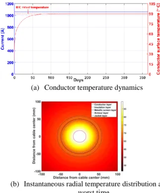
The results for the dynamic analysis under the aforementioned conditions are presented in the Figure 5. In the Figure 5a, the conductor temperature time series calculated at terminals of the offshore substation (curve red line), is showed along with the input current (blue line). It can be appreciated how the steady state value converges to 90℃ after approximately 116 days of operation. Refer to the Figure 5b to see the instantaneous temperature geometrical distribution along the cable cross section in the most critical hour of the year; it is noticeable that for these operating conditions the jacket temperature is around 60℃, value which can be used for recalibrating the model in real- time with on-line measuring, if dynamic temperature control systems should to be implemented.

From these results two main outcomes must be highlighted:

First, the dedicated dynamic model is validated under steady state conditions, since the resultant conductor temperature is consistent, and accurate compared to the one calculated by means of the static rating equation of [4]

(straight red line). Second, the slow time constant of the system is evident: it requires around 116 days overcoming the thermal transients, and reaching the steady state temperature. This shows that the static equation omits an important part regarding the system settling time, and points out a clear potential for allowing the operation of the cable beyond the nominal power for some periods.

(a) Conductor temperature dynamics

(b) Instantaneous radial temperature distribution at worst time

Figure 5: Dynamic temperature prediction of the cable under analysis for rated conditions evaluated at OSS terminals: 450 𝑀𝑊 and 𝜃𝑎𝑚𝑏 = 20℃.

Other important aspect not included in [4] and other references in the literature, is the effect of the capacitive currents on the cable temperature dynamic analysis and

5 lifetime. Simulations have been implemented at the onshore connection point terminals to calculate the DTP. The steady state temperature reached by the conductor is around 95℃

after roughly 120 days of operation; the current increase at this physical point causes a greater final temperature, a faster system response and similar settling time than the calculations performed at OSS’s terminals. These results reflect a key aspect to take into consideration when sizing a cable, which is the non-uniform degradation of the cable along its longitudinal dimension due to the current distribution. In this case, the terminal at onshore terminals will exhibit a faster degradation rate, and consequently, shorter lifetime expectancy due to accumulation of the capacitive currents.

After the evaluation of the model under rated conditions, the simulation for time-variable inputs is carried out. The main two stochastic variables involved in the analysis are showed in the Figure 6 and Figure 7. The Figure 6 presents the time variation of the external temperature at a particular OWF location (bottom of the seabed); the variable exhibits a considerable temperature spread between −1℃ and 21.5℃.

Likewise, for the same OWF location, the power generation time series has been simulated; the power histogram is available in the Figure 7, where it can be appreciated that 39.5% of the time the power generated falls in the 0.9 − 1.0 𝑝. 𝑢 bin of power (typical value for offshore sites).

Figure 6: 2-meters above-sea temperature time series.

Figure 7: Power generation histogram.

The Figure 8 shows the dynamic state of the conductor temperature, which exhibits a maximum temperature of 80℃. The main outcome is the considerable available margin of cable use exploitation, given that this value is lower than the recommended by manufacturers (90℃).

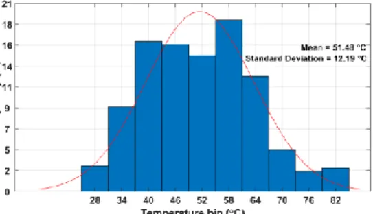
Indeed, it is still a conservative criterion to limit the conductor instantaneous maximum temperature to 90℃, considering that in other time periods the temperature can drop down to 30 ℃. In fact, as it can be seen in the Figure

9, less than 1% of the time the conductor experiences the peak temperature, and a value of 51.5 ℃ represents the mean in a normal pdf function.

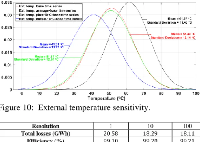
Regarding the effect of the external temperature over the dynamic performance of the cable, Figure 10 presents the results when considering a constant average profile (green line), a variable profile with positive 10℃ instantaneous deviation (black line), and variable profile with negative 10℃ instantaneous deviation (blue line), respect to the profile presented in the Figure 6 (base case, red line).

Figure 8: Dynamic temperature prediction of the cable under analysis for time variable conditions evaluated at onshore terminals.

The average-base profile presents a similar behaviour to the base case, however with a slight decrease on mean, and peak magnitudes. On the other hand, the plus-10℃-base profile, causes a greater mean value and lower spread on the temperature distribution, in contrast to the minus-10℃-base profile, which exhibits an opposite behaviour. In terms of temperature magnitude, the effects of the variation seems to cause a linear shift on the conductor temperature, however, it is more interesting to see the non-linear change on the standard deviation, which ultimately will cause a different degradation on the insulation material, and consequently, a pronounced impact over the lifetime of the cable. The effects are more complex when considering the combined changes on magnitude and spread. Lifetime models also demonstrate a considerable impact over the insulation ageing with, in principle, small variations of temperature magnitude.

Figure 9: Conductor surface temperature histogram and pdf fitting under base external temperature conditions.

Figure 10: External temperature sensitivity.

Resolution 1 10 100

Total losses (GWh) 20.58 18.29 18.11

Efficiency (%) 99.10 99.20 99.21

Computing time (h) 0.085 0.53 5.76

Table 1: Cable performance evaluation

Table 1 shows the results of the last block of the methodology (Figure 2), which applies the Equation (4), varying the cable sections 𝑙𝐷_𝑇, and fixing ℎ = 8760 ℎ𝑜𝑢𝑟𝑠 (carried out for the year with highest capacity factor). As it can be noted, after 10 sections, total losses variation is negligible and unnecessary in terms of the computing time growth, indeed, the efficiency variation is derisory;

therefore, a rough approximation of ten sections is more than acceptable. It is important to remark the value of an accurate total electric losses estimation for financial analysis, with more than 0.1% error in the losses calculations.

5 Conclusions

This paper introduced a comprehensive methodology, combining different concepts, to optimally size offshore wind farms AC export cables. The focus of this work has been to describe the basics on the formulated approach, and exploring the application of a TEE model for Dynamic Temperature Prediction (DTP).

The currently used criterion for sizing cables in weather- based systems generations is obsolete and over- conservative, results on this paper point out the over- dimensioning of cables by applying such methodologies, from a point of view of insulation ageing. Additionally, the effects of the variation of seabed temperature have been quantified, and the importance of accurate gathering of data is stressed by performing a sensitivity analysis.

Future work will present the full application of the methodology, in conceptual terms, and by analysing specific case studies.

Acknowledgements

The research leading to these results has received funding from the Baltic InteGrid Project (http://www.baltic- integrid.eu/).

References

[1] GWEC, “Global Wind Report. Annual Market Update 2017,” Glob. Wind Energy Counc., p. 72, 2017.

[2] X. Sun, D. Huang, and G. Wu, “The current state of offshore wind energy technology development,”

Energy, vol. 41, no. 1, pp. 298–312, 2012.

[3] ReNEWS, “Rampion suffers cable fault,” 2017.

[Online]. Available:

http://renews.biz/105889/rampion-suffers-cable- fault/.

[4] I. Standard, “IEC-60287-1-1: Electric cables - Calculation of the current rating,” 2001.

[5] V. K. Agarwal et al., “The Mysteries of Multifactor Ageing,” IEEE Electr. Insul. Mag., vol. 11, no. 3, pp. 37–43, 1995.

[6] P. Sørensen, M. Litong-palima, A. N. Hahman, S.

Heunis, M. Ntusi, and J. C. Hansen, “Wind power variability and power system reserves in South Africa,” J. Energy, vol. 29, no. 1, pp. 59–71, 2018.

[7] R. Olsen, G. J. Anders, J. Holboell, and U. S.

Gudmundsdottir, “Modelling of dynamic transmission cable temperature considering soil- specific heat, thermal resistivity, and precipitation,”

IEEE Trans. Power Deliv., vol. 28, no. 3, pp. 1909–

1917, 2013.

[8] R. S. Olsen, J. Holboll, and U. S. Gudmundsdottir,

“Dynamic temperature estimation and real time emergency rating of transmission cables,” IEEE Power Energy Soc. Gen. Meet., pp. 1–8, 2012.

[9] T. Kvarts, “Systematic Description of Dynamic Load for Cables for Offshore Wind Farms . Method and Experience,” no. August 2016, 2018.

[10] J. J. Grainger and W. D. J. Stevenson, Power System Analysis. 1994.

[11] G. Mazzanti and G. C. Montanari, “A comparison between XLPE and EPR as insulating materials for HV cables,” IEEE Trans. Power Deliv., vol. 12, no.

1, pp. 15–26, 1997.

[12] M. Miner, “Cumulative fatigue damage,” J. Appl.

Mech., vol. 12, no. 3, pp. A159--A164, 1945.

[13] H. Wire, “Miner’s Rule and Cumulative Damage Models,” 2018. [Online]. Available:

https://www.weibull.com/hotwire/issue116/hottopi cs116.htm.

[14] H. Brakelmann, “Loss determination for long three- phase high-voltage submarine cables,” Eur. Trans.

Electr. Power, vol. 13, no. 3, pp. 193–197, 2003.

[15] J. L. Aznarte and N. Siebert, “Dynamic Line Rating Using Numerical Weather Predictions and Machine Learning: A Case Study,” IEEE Trans. Power Deliv., vol. 32, no. 1, pp. 335–343, 2017.