Lectures on Supersymmetry

(1)

Lectures on Supersymmetry

Matteo Bertolini

SISSA

June 9, 2021

(2)

Foreword

This is a write-up of a course on Supersymmetry I have been giving for several years to first year PhD students attending the curriculum in Theoretical Particle Physics at SISSA, the International School for Advanced Studies of Trieste.

There are several excellent books on supersymmetry and many very good lecture courses are available on the archive. The ambition of this set of notes is not to add anything new in this respect, but to offer a set of hopefully complete and self- consistent lectures, which start from the basics and arrive to some of the more recent and advanced topics. The price to pay is that the material is pretty huge.

The advantage is to have all such material in a single, possibly coherent file, and that no prior exposure to supersymmetry is required.

There are many topics I do not address and others I only briefly touch. In particular, I discuss only rigid supersymmetry (mostly focusing on four space-time dimensions), while no reference to supergravity is given. Moreover, this is a theoretical course and phenomenological aspects are only briefly sketched. One only chapter is dedicated to present basic phenomenological ideas, including a bird eyes view on models of gravity and gauge mediation and their properties, but a thorough discussion of phenomenological implications of supersymmetry would require much more.

There is no bibliography at the end of the file. However, each chapter contains its own bibliography where the basic references (mainly books and/or reviews available on-line) I used to prepare the material are reported – including explicit reference to corresponding pages and chapters, so to let the reader have access to the original font (and to let me give proper credit to authors).

I hope this effort can be of some help to as many students as possible!

Disclaimer: I expect the file to contain many typos and errors. Everybody is welcome to let me know them, dialing at matteo.bertolini@sissa.it. Your help will be very much appreciated.

(3)

1 Supersymmetry: a bird eyes view

Coming years could represent a new era of unexpected and exciting discoveries in high energy physics, since a long time. For one thing, the CERN Large Hadron Collider (LHC) has been operating for some time, now, and many experimental data have already being collected. So far, the greatest achievement of the LHC has been the discovery of the missing building block of the Standard Model, the Higgs particle (or, at least, a particle which most likely is the Standard Model Higgs particle). On the other hand, no direct evidence of new physics beyond the Standard Model has been found, yet. Still, there are several reasons to believe that new physics should in fact show-up at, or about, the TeV scale.

The most compelling scenario for physics beyond the Standard Model (BSM) is supersymmetry. For this reason, knowing what is supersymmetry is rather important for a high energy physicist, nowadays. Understandinghowsupersymmetry can be realized (and then spontaneously broken) in Nature, is in fact one of the most important challenges theoretical high energy physics has to confront with. This course provides an introduction to such fascinating subject.

Before entering into any detail, in this first lecture we just want to give a brief overview on what is supersymmetry and why is it interesting to study it. The rest of the course will try to provide (much) more detailed answers to these two basic questions.

Disclaimer: The theory we are going to focus our attention in the (more than) three-hundred pages which follow, can be soon proved to be the correct mathematical framework where to understand high energy physics at the TeV scale, and become a piece of basic knowledge any particle physicist should have. But it can very well be that BSM physics is more subtle and Nature not so kind to make supersymmetry be realized at low enough energy that we can make experiment of. Or, it can also be that all this will eventually turn out to be just a purely academic exercise about a theory that nothing has to do with Nature. An elegant way mankind has worked out to describe in an unique and self-consistent way elementary particle physics, which however is not the one chosen by Nature (but can we ever safely say so?). As I will briefly outline below, and discuss in more detail in the second part of this course, even in such a scenario... studying supersymmetry and its fascinating properties might still be helpful and instructive in many respects.

(8)

1.1 What is supersymmetry?

Supersymmetry (SUSY) is a space-time symmetry mapping particles and fields of integer spin (bosons) into particles and fields of half integer spin (fermions), and viceversa. The generatorsQ act as

Q|F ermioni = |Bosoni and viceversa (1.1) From its very definition, this operator has two obvious but far-reaching properties that can be summarized as follows:

• It changes the spin of a particle (meaning that Q transforms as a spin-1/2 particle) and hence its space-time properties. This is why supersymmetry is not an internal symmetry but a space-time symmetry.

• In a theory where supersymmetry is realized, each one-particle state has at least a superpartner. Therefore, in a SUSY world, instead of single particle states, one has to deal with (super)multiplets of particle states.

Supersymmetry generators have specific commutation properties with other generators. In particular:

• Qcommutes with translations and internal quantum numbers (e.g. gauge and global symmetries), but it does not commute with Lorentz generators

[Q, P_µ] = 0 , [Q, G] = 0 , [Q, M_µν]6= 0 . (1.2) This implies that particles belonging to the same supermultiplet have different spin but same mass and same quantum numbers.

A supersymmetric field theory is a set of fields and a Lagrangian which exhibit such a symmetry. As ordinary field theories, supersymmetric theories describe particles and interactions between them: SUSY manifests itself in the specific particle spectrum a theory enjoys, and in the way particles interact between themselves.

A supersymmetric model which is covariant under general coordinate transformations is called supergravity (SUGRA) model. In this respect, a non-trivial fact, which again comes from the algebra, in particular from the (anti)commutation relation

{Q,Q¯} ∼P_µ , (1.3)

(9)

is that having general coordinate transformations is equivalent to have local SUSY, the gauge mediator being a spin 3/2 particle, the gravitino. Hence local supersymmetry and General Relativity are intimately tied together.

One can have theories with different number of SUSY generators Q: Q^I I = 1, ..., N. The number of supersymmetry generators, however, cannot be arbitrarily large. The reason is that any supermultiplet contains particles with spin at least as large as ¹₄N. Therefore, to describe local and interacting theories, N can be at most as large as 4 for theories with maximal spin 1 (gauge theories) and as large as 8 for theories with maximal spin 2 (gravity). Thus stated, this statement is true in 4 space-time dimensions. Equivalent statements can be made in higher/lower dimensions, where the dimension of the spinor representation of the Lorentz group is larger/smaller (for instance, in 10 dimensions, which is the natural dimension where superstring theory lives, the maximum allowedN is 2). What really matters is the number of single state supersymmetry generators, which is an invariant, dimension- independent statement.

Finally, notice that since supersymmetric theories automatically accomodate both bosons and fermions, SUSY looks like the most natural framework where to formulate a theory able to describe matter and interactions in a unified way.

1.2 What is supersymmetry useful for?

Let us briefly outline a number of reasons why it might be meaningful (and useful) to have such a bizarre and unconventional symmetry actually realized in Nature.

i. Theoretical reasons.

• What are the more general allowed symmetries of the S-matrix? In 1967 Cole- man and Mandula proved a theorem which says that in a generic quantum field theory, under a number of (very reasonable and physical) assumptions, like locality, causality, positivity of energy, finiteness of number of particles, etc..., the only possible continuos symmetries of the S-matrix are those gener- ated by Poincar´e group generators, P_µ andM_µν, plus some internal symmetry group G (where G is a semi-simple group times abelian factors) commuting with them

[G, P_µ] = [G, M_µν] = 0 . (1.4) In other words, the most general symmetry group enjoyed by the S-matrix is

(10)

Poincar´e × Internal Symmetries

The Coleman-Mandula theorem can be evaded by weakening one or more of its assumptions. One such assumptions is that the symmetry algebra only in- volvescommutators, all generators being bosonicgenerators. This assumption does not have any particular physical reason not to be relaxed. Allowing for fermionic generators, which satisfy anti-commutation relations, it turns out that the set of allowed symmetries can be enlarged. More specifically, in 1975 Haag, Lopuszanski and Sohnius showed that supersymmetry (which, as we will see, is a very specific way to add fermionic generators to a symmetry algebra) is the only possible such option. This makes the Poincar´e group becoming Su- perPoincar´e. Therefore, the most general symmetry group the S-matrix can enjoy turns out to be

SuperPoincar´e × Internal Symmetries

From a purely theoretical view point, one could then well expect that Nature might have realized all possible kind of allowed symmetries, given that we already know this is indeed the case (cf. the Standard Model) for all known symmetries, but supersymmetry.

• The history of our understanding of physical laws is an history of unification.

The first example is probably Newton’s law of universal gravitation, which says that one and the same equation describes the attraction a planet exert on another planet and on... an apple! Maxwell equations unify electromagnetism with special relativity. Quantumelectrodynamics unifies electrodynamics with quantum mechanics. And so on and so forth, till the formulation of the Stan- dard Model which describes in an unified way all known non-gravitational interactions. Supersymmetry (and its local version, supergravity), is the most natural candidate to complete this long journey. It is a way not just to describe in a unified way all known interactions, but in fact to describe matter and radiation all together. This sounds compelling, and from this view point it sounds natural studying supersymmetry and its consequences.

• Finally, I cannot resist to add one more reason as to why one could expect that supersymmetry is out there, after all. Supersymmetry is possibly one of the two more definite predictions of String Theory, the other being the existence of extra-dimensions.

(11)

Note: all above arguments suggest that supersymmetry maybe realized as a symmetry in Nature. However, none of such arguments gives any obvious indication on the energy scale supersymmetry might show-up. This can be very high, in fact.

Below, we will present a few more arguments, more phenomenological in nature, which deal, instead, with such an issue and actually suggest that low energy supersymmetry (as low as TeV scale or slightly higher) would be the preferred option.

ii. Elementary Particle theory point of view.

• Naturalness and the hierarchy problem. Three out of four of the fundamental interactions among elementary particles (strong, weak and electromagnetic) are described by the Standard Model (SM). The typical scale of the SM, the electroweak scale, is

M_ew∼250 GeV ⇔L_ew ∼10⁻¹⁶ mm . (1.5) The SM is very well tested up to such energies. This cannot be the end of the story, though: for one thing, at high enough energies, as high as the Planck scale M_pl, gravity becomes comparable with other forces and cannot be neglected in elementary particle interactions. At some point, we need a quantum theory of gravity. Actually, the fact that M_ew/M_pl << 1 calls for new physics at a much lower scale. One way to see this, is as follows. The Higgs potential reads

V(H)∼µ²|H|²+λ|H|⁴ where µ² <0 . (1.6) Experimentally, the minimum of such potential,hHi=p

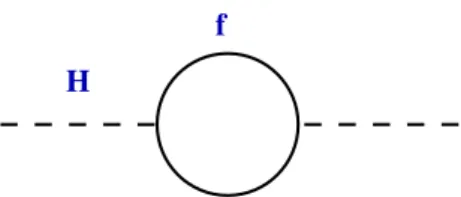
−µ²/2λ, is at around 174GeV. This implies that the bare mass of the Higgs particle is roughly around 100 GeV or so, m²_H = −µ² ∼ (100GeV)². What about radiative corrections? Scalar masses are subject to quadratic divergences in perturbation theory. The SM fermion coupling −λ_fHf f¯ induces a one-loop correction to the Higgs mass as

∆m²_H ∼ −2λ²_f Λ² (1.7)

due to the diagram in Figure 1.1. The UV cut-off Λ should then be naturally around the TeV scale in order to protect the Higgs mass, and the SM should then be seen as an effective theory valid atE < M_eff ∼TeV.

What can be the new physics beyond such scale and how can such new physics protect the otherwise perturbative divergent Higgs mass? New physics, if any,

(12)

H

f

Figure 1.1: One-loop radiative correction to the Higgs mass due to fermion couplings.

may include many new fermionic and bosonic fields, possibly coupling to the SM Higgs. Each of these fields will give radiative contribution to the Higgs mass of the kind above, hence, no matter what new physics will show-up at high energy, the natural mass for the the Higgs field would always be of order the UV cut-off of the theory, generically around∼M_pl. We would need a huge fine-tuning to get it stabilized at ∼ 100GeV (we now know that the physical Higgs mass is at 125 GeV, in fact)! This is known as thehierarchy problem: the experimental value of the Higgs mass is unnaturally smaller than its natural theoretical value.

In principle, there is a very simple way out of this. This resides in the fact that (as you should know from your QFT course!) scalar couplings provide one-loop radiative contributions which are opposite in sign with respect to fermions.

Suppose there exist some new scalar, S, with Higgs coupling −λ_S|H|²|S|². Such coupling would also induce corrections to the Higgs mass via the one- loop diagram in Figure 1.2.

S

H

Figure 1.2: One-loop radiative correction to the Higgs mass due to scalar couplings.

Such corrections would have opposite sign with respect to those coming from fermion couplings

∆m²_H ∼ λ_S Λ² . (1.8)

Therefore, if the new physics is such that each quark and lepton of the SM were accompanied by two complex scalars having the same Higgs couplings of the quark and lepton, i.e. λ_S = |λ_f|², then all Λ² contributions would automatically cancel, and the Higgs mass would be stabilized at its tree level value!

(13)

Such conspiracy, however, would be quite ad hoc, and not really solving the fine-tuning problem mentioned above; rather, just rephrasing it. A natural thing to invoke to have such magic cancellations would be to have a symmetry protecting m_H, right in the same way as gauge symmetry protects the mass- lessness of spin-1 particles. A symmetry imposing to the theory the correct matter content (and couplings) for such cancellations to occur. This is exactly what supersymmetry is: in a supersymmetric theory there are fermions and bosons (and couplings) just in the right way to provideexact cancellation between diagrams like the ones above. In summary, supersymmetry is a very natural and economic way (though not the only possible one) to solve the hierarchy problem.

Known fermions and bosons cannot be partners of each other. For one thing, we do not observe any degeneracy in mass in elementary particles that we know. Moreover, and this is possibly a stronger reason, quantum numbers do not match: gauge bosons transform in the adjoint reps of the SM gauge group while quarks and leptons in the fundamental or singlet reps. Hence, in a supersymmetric world, each SM particle should have a (yet not observed!) supersymmetric partner, usually dubbed sparticle. Roughly, the spectrum should be as follows

SM particles SUSY partners gauge bosons gauginos quarks, leptons scalars

Higgs higgsino

Notice: the (down) Higgs has the same quantum numbers as the scalar partner of neutrino and leptons, sneutrino and sleptons respectively, (H_d⁰, H_d⁻)↔ (˜ν,e˜_L). Hence, one can imagine that the Higgs is in fact a sparticle. This cannot be. In such scenario, there would be phenomenological problems, e.g.

lepton number violation and (at least one) neutrino mass in gross violation of experimental bounds.

In summary, the world we already had direct experimental access to, is not supersymmetric. If at all realized, supersymmetry should be a (spontaneously) broken symmetry in the vacuum state chosen by Nature. However, in order to solve the hierarchy problem without fine-tuning this scale should be lower than (or about) 1 TeV. Including lower bounds from present day experiments,

(14)

it turns out that the SUSY breaking scale should be in the following energy range

100 GeV≤SUSY breaking scale≤1000 GeV .

This is the basic reason why it is believed SUSY to show-up at the LHC.

Let us notice that these bounds are just a crude and rough estimate, as they depend very much on the specific SSM one is actually considering. In particular, the upper bound can be made higher by enriching the structure of the SSM in various ways, as well as defining the concept of naturalness in a less restricted way. There are ongoing discussions on these aspects nowadays, including the idea that naturalness should not be taken as a such important guiding principle, at least in this context.

• Gauge coupling unification. There is another reason to believe in supersymmetry; possibly stronger, from a phenomenological point of view, then that provided by the hierarchy problem. Forget about supersymmetry for a while, and consider the SM as it stands. Interesting enough, besides the EW scale, the SM contains in itself a new scale of order 10¹⁵GeV. The three SM gauge couplings run according to RG equations like

4π

g_i²(µ) = b_i 2πln µ

Λi

i= 1,2,3 . (1.9)

At the EW scale, µ = M_Z, there is a hierarchy between them, g₁(M_Z) <

g₂(M_Z) < g₃(M_Z). But RG equations make this hierarchy changing with the energy scale. In fact, supposing there are no particles other than the SM ones, at a much higher scale, M_{GU T} ∼ 10¹⁵GeV, the three couplings tend to meet! This naturally calls for a Grand Unified Theory (GUT), where the three interactions are unified in a single one, two possible GUT gauge groups being SU(5) and SO(10). The symmetry breaking pattern one should have in mind would then be as follows

SU(5) → SU(3)×SU(2)_L×U(1)_Y →SU(3)×U(1)_em

φ H

where φ is an heavy Higgs inducing spontaneous symmetry breaking at energies M_{GU T} ∼10¹⁵GeV, and H the SM light Higgs, inducing EW spontaneous symmetry breaking around the TeV scale. This idea poses several problems.

(15)

First, there is a new hierarchy problem (generically, the SM Higgs mass is expected to get corrections from the heavy Higgsφ). Second, there is a proton decay problem: some of the additional gauge bosons mediate baryon number violating transitions, allowing processes as p→e⁺+π₀. This makes the proton not fully stable and it turns out that its expected lifetime in such GUT framework is violated by present experimental bounds. On a more theoretical side, if we do not allow for new particles besides the SM ones to be there at some intermediate scale, the three gauge couplings only approximately meet.

The latter is an unpleasant feature: small numbers are unnatural from a theoretical view point, unless there are specific reasons (as symmetries) justifying their otherwise unnatural smallness.

Remarkably, making the GUT supersymmetric (SGUT) solves all of these problems in a glance! If one just allows for the minimal supersymmetric extension of the SM spectrum, known as MSSM, the three gauge couplings exactly meet, and the GUT scale is raised enough to let proton decay rate being compatible with present experimental bounds.

10

−1

−2

SU(2)

U(1)

Coupling

Energy

Coupling

Energy 10¹⁶

10 10⁻¹

−2

SU(3)

U(1) SU(2)

1016 SU(3)

Standard Model ... + SUSY

Disclaimer: the MSSM is not the only possible option for supersymmetry beyond the SM, just the most economic one. In the MSSM one just adds a superpartner to each SM particle, therefore introducing the higgsino, the wino, the zino, together with all squarks and sleptons, and no more. [There is in fact an exception. To have a meaningful model one has to double the Higgs sector, and have two Higgs doublets. One reason for that is gauge anomaly cancellation: the higgsinos are fermions in the fundamental rep of SU(2)_Lhence two of them are needed, with opposite hypercharge, not to spoil

(16)

the anomaly-free properties of the SM. A second reason is that in the SM the field H gives mass to down quarks and charged leptons while its charge conjugate,H^c(∼H) gives mass to up quarks. As we will see, in a SUSY model¯ H¯ cannot enter in the potential, which is a function of H, only. Therefore, in a supersymmetric scenario, to give mass to up quarks one needs a second, independent Higgs doublet.] There exist many non-minimal supersymmetric extensions of the Standard Model (which, in fact, are in better shape against experimental constraints with respect to the MSSM). One can in principle construct any SSM one likes. In doing so, however, several constraints are to be taken into account. For example, it is not so easy to make such non- minimal extensions keeping the nice exact gauge coupling unification enjoyed by the MSSM.

The important lesson we get out of all this discussion can be summarized as follows: in a SUSY quantum field theory radiative corrections are suppressed. Quan- tities that are small (or vanishing) at tree level tend to remain so at quantum level.

This is at the basis of the solutions of all problems we mentioned: the hierarchy problem, the proton life-time, and gauge couplings unification.

iii. Supersymmetry and Cosmology.

• Let me briefly mention yet another context where supersymmetry might play an important role. There are various evidences which indicate that around 26% of the energy density in the Universe should be made of dark matter, i.e. non-luminous and non-baryonic matter. The only SM candidates for dark matter are neutrinos, but they are disfavored by available experimental data.

Supersymmetry provides a valuable and very natural dark matter candidate:

the neutralino. Neutralinos are mass eigenstates of a linear superposition of the SUSY partners of the neutral Higgs and of the SU(2) and U(1) neutral gauge bosons

χ_i =α_i1B˜⁰+α_i2W˜⁰+α_i3H˜_u⁰+α_i4H˜_d⁰ . (1.10) Interestingly, in most SUSY frameworks the neutralino is the lightest supersymmetric particle (LSP), and fully stable, as a dark matter candidate should be.

iv. Supersymmetry as atheoretical laboratoryfor strongly coupled gauge dynamics.

(17)

• What if supersymmetry will turn out not to be the correct theory to describe (low energy) beyond the SM physics? Or, worse, what if supersymmetry will turn out not to be realized at all, in Nature (something we could hardly ever being able to prove, in fact)? Interestingly, there is yet another reason which makes it worth studying supersymmetric theories, independently from the role supersymmetry might or might not play as a theory describing high energy physics.

Let us consider non-abelian gauge theories, which strong interactions are an example of. Every time a non-abelian gauge group remains unbroken at low energy, we have to deal with strong coupling. The typical questions one should try and answer (in QCD or similar theories) are:

– The bare Lagrangian is described in terms of quark and gluons, which are UV degrees of freedom. Which are the IR (light) degrees of freedom of QCD? What is the effective Lagrangian in terms of such degrees of freedom?

– Strong coupling physics is very rich. Typically, one has to deal with phenomena like confinement, charge screening, the generation of a mass gap, etc.... Is there any theoretical understanding of such phenomena?

– The QCD vacuum is populated by vacuum condensates of fermion bilin- ears, hΩ|ψψ¯ |Ωi 6= 0, which induce chiral symmetry breaking. What is the microscopic mechanism behind this phenomenon?

Most of the IR properties of QCD have eluded so far a clear understanding, since we lack analytical tools to deal with strong coupling dynamics. Most results come from lattice computations, but these do not furnish a theoretical, first principle understanding of the above phenomena. Moreover, they are formulated in Euclidean space and are not suited to discuss, e.g. transport properties.

Because of their nice renormalization properties, supersymmetric theories are more constrained than ordinary field theories and let one have a better control on strong coupling regimes, sometime. Therefore, one might hope to use them as toy models where to study properties of more realistic theories, such as QCD, in a more controlled way. Indeed, as we shall see, supersymmetric theories do provide examples where some of the above strong coupling effects can be studied exactly! This is possible due to powerful non-renormalizations

(18)

theorems supersymmetric theories enjoy, and because of a very special property of supersymmetry, known as holomorphy, which in certain circumstances lets one compute several non-perturbative contributions to the Lagrangian. We will spend a sizeable amount of time discussing these issues in the second part of this course.

This is all we wanted to say in this short introduction, that should be regarded just as an invitation to supersymmetry and its fascinating world. Let us end by just adding a curious historical remark. Supersymmetry did not first appear in ordinary four-dimensional quantum field theories but in string theory, at the very beginning of the seventies. Only later it was shown to be possible to have supersymmetry in ordinary quantum field theories.

1.3 Some useful references

The list of references in the literature is endless. I list below few of them, including books as well as some archive-available reviews. Some of these references may be better than others, depending on the specific topic one is interested in (and on per- sonal taste). In preparing these lectures I have used most of them, some more, some less. At the end of each lecture I list those references (mentioning corresponding chapters and/or pages) which have been used to prepare it. This will let students having access to the original font, and me give proper credit to authors.

1. Historical references

• J. Wess and J. Bagger

Supersymmetry and supergravity

Princeton, USA: Univ. Pr. (1992) 259 p.

• P. C. West

Introduction to supersymmetry and supergravity Singapore: World Scientific (1990) 425 p.

• M. F. Sohnius

Introducing Supersymmetry Phys. Rep. 128 (1985) 2. More recent books

(19)

• S. Weinberg

The quantum theory of fields. Vol. 3: Supersymmetry Cambridge, UK: Univ. Pr. (2000) 419 p.

• J. Terning

Modern supersymmetry: Dynamics and duality Oxford, UK: Clarendon (2006) 324 p.

• M. Dine

Supersymmetry and string theory: Beyond the standard model Cambridge, UK: Cambridge Univ. Pr. (2007) 515 p.

• H.J. M¨uller-Kirsten and A. Wiedemann Introduction to Supersymmetry

Singapore: World Scientific (2010) 439 p.

3. On-line reviews: bases

• J. D. Lykken

Introduction to Supersymmetry arXiv:hep-th/9612114

• S. P. Martin

A Supersymmetry Primer arXiv:hep-ph/9709356

• A. Bilal

Introduction to supersymmetry arXiv:hep-th/0101055

• J. Figueroa-O’Farrill

BUSSTEPP Lectures on Supersymmetry arXiv:hep-th/0109172

• M. J. Strassler

An Unorthodox Introduction to Supersymmetric Gauge Theory arXiv:hep-th/0309149

• R. Argurio, G. Ferretti and R. Heise

An introduction to supersymmetric gauge theories and matrix models Int. J. Mod. Phys. A 19 (2004) 2015 [arXiv:hep-th/0311066]

4. On-line reviews: advanced topics

(20)

• K. A. Intriligator and N. Seiberg

Lectures on supersymmetric gauge theories and electric-magnetic duality Nucl. Phys. Proc. Suppl. 45BC (1996) 28 [arXiv:hep-th/9509066]

• A. Bilal

Duality in N=2 SUSY SU(2) Yang-Mills Theory: A pedagogical introduction to the work of Seiberg and Witten

arXiv:hep-th/9601007

• M. E. Peskin

Duality in Supersymmetric Yang-Mills Theory arXiv:hep-th/9702094

• M. Shifman

Non-Perturbative Dynamics in Supersymmetric Gauge Theories Prog. Part. Nucl. Phys. 39 (1997) 1 [arXiv:hep-th/9704114]

• P. Di Vecchia

Duality in supersymmetric N = 2,4 gauge theories arXiv:hep-th/9803026

• M. J. Strassler The Duality Cascade arXiv:hep-th/0505153

• P. Argyres

Lectures on Supersymmetry

available at http://www.physics.uc.edu/~argyres/661/index.html 5. On-line reviews: supersymmetry breaking

• G. F. Giudice and R. Rattazzi

Theories with Gauge-Mediated Supersymmetry Breaking Phys. Rept. 322 (1999) 419 [arXiv:hep-ph/9801271]

• E. Poppitz and S. P. Trivedi

Dynamical Supersymmetry Breaking

Ann. Rev. Nucl. Part. Sci. 48 (1998) 307[arXiv:hep-th/9803107]

• Y. Shadmi and Y. Shirman

Dynamical Supersymmetry Breaking

Rev. Mod. Phys. 72 (2000) 25 [arXiv:hep-th/9907225]

(21)

• M. A. Luty

2004 TASI Lectures on Supersymmetry Breaking arXiv:hep-th/0509029

• Y. Shadmi

Supersymmetry breaking arXiv:hep-th/0601076

• K. A. Intriligator and N. Seiberg Lectures on Supersymmetry Breaking

Class. Quant. Grav. 24 (2007) S741 [arXiv:hep-ph/0702069]

(22)

2 The supersymmetry algebra

In this lecture we introduce the supersymmetry algebra, which is the algebra encoding the set of symmetries a supersymmetric theory should enjoy.

2.1 Lorentz and Poincar´ e groups

The Lorentz group SO(1,3) is the subgroup of matrices Λ of GL(4, R) with unit determinant, detΛ = 1, and which satisfy the following relation

Λ^TηΛ =η (2.1)

whereη is the (mostly minus in our conventions) flat Minkowski metric

ηµν = diag(+,−,−,−) . (2.2) The Lorentz group has six generators (associated to space rotations and boosts) enjoying the following commutation relations

[Ji, Jj] =iijkJk , [Ji, Kj] =iijkKk , [Ki, Kj] =−iijkJk . (2.3) Notice that while theJ_i are hermitian, the boostsK_i are anti-hermitian, this being related to the fact that the Lorentz group is non-compact (topologically, the Lorentz group isR³×S₃/Z², the non-compact factor corresponding to boosts and the doubly connected S₃/Z² corresponding to rotations). In order to construct representations of this algebra it is useful to introduce the following complex linear combinations of the generators J_i and K_i

J_i^± = 1

2(J_i±iK_i) , (2.4)

where now theJ_i^± are hermitian. In terms of J_i^± the algebra (2.3) becomes

[J_i^±, J_j^±] =i_ijkJ_k^± , [J_i^±, J_j^∓] = 0 . (2.5) This shows that the Lorentz algebra is equivalent to twoSU(2) algebras. As we will see later, this simplifies a lot the study of the representations of the Lorentz group, which can be organized into (couples of) SU(2) representations. This isomorphism comes from the theory of Lie Algebra which says that at the level of complex algebras SO(4)'SU(2)×SU(2) . (2.6)

(23)

In fact, the Lorentz algebra is a specific real form of that of SO(4). This difference can be seen from the defining commutation relations (2.3): for SO(4) one would have had a plus sign on the right hand side of the third such commutation relations.

This difference has some consequence when it comes to study representations. In particular, while in Euclidean space all representations are real or pseudoreal, in Minkowski space complex conjugation interchanges the two SU(2)’s. This can also be seen at the level of the generatorsJ_i^±. In order for all rotation and boost param- eters to be real, one must take all the J_i and K_i to be imaginary and hence from eq. (2.4) one sees that

(J_i^±)^∗ =−J_i^∓ . (2.7)

In terms of algebras, all this discussion can be summarized noticing that for the Lorentz algebra the isomorphism (2.6) changes into

SO(1,3)'SU(2)×SU(2)^∗ . (2.8) For later purpose let us introduce a four-vector notation for the Lorentz generators, in terms of an anti-symmetric tensorM_µν defined as

M_µν =−M_νµ with M_0i =K_i and M_ij =_ijkJ_k , (2.9) whereµ= 0,1,2,3. In terms of such matrices, the Lorentz algebra reads

[Mµν, Mρσ] =−iηµρMνσ−iηνσMµρ+iηµσMνρ+iηνρMµσ . (2.10) Another useful relation one should bear in mind is the relation between the Lorentz group andSL(2,C), the group of 2×2 complex matrices with unit determinant. More precisely, there exists a homomorphism betweenSL(2,C) and SO(1,3), which means that for any matrix A ∈ SL(2,C) there exists an associated Lorentz matrix Λ, and that

Λ(A) Λ(B) = Λ(AB) , (2.11)

where A and B are SL(2,C) matrices. This can be proved as follows. Lorentz transformations act on four-vectors as

x^0µ= Λ^µ_νx^ν , (2.12)

where the matrices Λ’s are a representation of the generators M_µν defined above.

Let us introduce 2×2 matrices σ_µ where σ₀ is the identity matrix and σ_i are the Pauli matrices defined as

σ₁ = 0 1 1 0

!

, σ₂ = 0 −i i 0

!

, σ₃ = 1 0 0 −1

!

. (2.13)

(24)

Let us also define the matrices with upper indices, σ^µ, as

σ^µ= (σ⁰, σⁱ) = (σ₀,−σ_i) . (2.14) The matricesσ_µ are a complete set, in the sense that any 2×2 complex matrix can be written as a linear combination of them. For every four-dimensional vector x^µ let us construct the 2×2 complex matrix

ρ:x^µ→x^µσ_µ=X . (2.15)

The matrix X is hermitian, since the Pauli matrices are hermitian, and has determinant equal to x^µx_µ, which is a Lorentz invariant quantity. Therefore, ρ is a map from Minkowski space to H, the space of 2×2 hermitian complex matrices

M₄ −→

ρ H . (2.16)

Let us now act on X with aSL(2,C) transformation A

A:X →AXA^† =X⁰ . (2.17)

This transformation preserves the determinant since detA = 1 and also preserves the hermicity of X since

X^0† = (AXA^†)^†=AX^†A^† =AXA^†=X⁰ . (2.18) ThereforeA is a map between H and itself

H −→

A H . (2.19)

We finally apply the inverse map ρ⁻¹ to X⁰ and get a four-vector x^0µ. The inverse map is defined as

ρ⁻¹ = 1

2Tr[• σ¯^µ] (2.20)

(where, as we will later see more rigorously, as a complex 2×2 matrix ¯σ^µ is the same asσµ). Indeed

ρ⁻¹X = 1

2Tr[Xσ¯^µ] = 1

2Tr[xνσ^νσ¯^µ] = 1

2Tr[σ^νσ¯^µ]xν = 1

22η^µνxν =x^µ . (2.21) Assembling everything together we then get a map from Minkowski space into itself via the following chain

M₄ −→_ρ H −→

A H −→

ρ⁻¹

M₄ x_ν −→

ρ x_νσ^ν −→

A Ax_νσ^νA^† −→

ρ⁻¹ 1

2Tr[Ax_νσ^νA^†σ¯^µ] =x^0µ (2.22)

(25)

This is nothing but a Lorentz transformation obtained by the SL(2,C) transformation A as

Λ^µ_ν(A) = 1

2Tr[¯σ^µA σ_νA^†] . (2.23) It is now a trivial exercise, provided eq. (2.23), to prove the homomorphism (2.11).

Notice that the relation (2.23) can in principle be inverted, in the sense that for a given Λ one can find a corresponding A ∈ SL(2,C). However, the relation is not an isomorphism, since it is double valued. The isomorphism holds between the Lorentz group and SL(2,C)/Z2 (in other words SL(2,C) is a double cover of the Lorentz group). This can be seen as follows. Consider the 2×2 matrix

M(θ) = e^−iθ/2 0 0 e^iθ/2

!

(2.24) which corresponds to a Lorentz transformation producing a rotation by an angle θ about the z-axis. Taking θ = 2π which corresponds to the identity in the Lorentz group, one getsM =−1 which is a non-trivial element ofSL(2,C). It then follows that the elements of SL(2,C) are identified two-by-two under a Z2 transformation in the Lorentz group. Note that thisZ2 identification holds also in Euclidean space:

at the level of groupsSU(2)×SU(2) =Spin(4), whereSpin(4) is a double cover of SO(4) as a group (it has an extraZ2).

The Poincar´e group is the Lorentz group augmented by the space-time transla- tion generators P_µ. In terms of the generatorsP_µ, M_µν the Poincar´e algebra reads

[P_µ, P_ν] = 0

[M_µν, M_ρσ] = −iη_µρM_νσ −iη_νσM_µρ+iη_µσM_νρ+iη_νρM_µσ (2.25) [Mµν, Pρ] = −iηρµPν+iηρνPµ .

2.2 Spinors and representations of the Lorentz group

We are now ready to discuss representations of the Lorentz group. Thanks to the isomorphism (2.8) they can be easily organized in terms of those of SU(2) which can be labeled by the spins. In this respect, let us introduce two-component spinors as the objects carrying the basic representations of SL(2,C). There exist two such representations. A spinor transforming in the self-representationMis a two complex component object

ψ = ψ₁ ψ₂

!

(2.26)

(26)

whereψ₁ and ψ₂ are complex Grassmann numbers, which transform under a matrix M ∈SL(2,C) as

ψ_α →ψ_α⁰ =Mα^βψ_β α, β = 1,2 . (2.27) The complex conjugate representation is defined from M^∗, where M^∗ means complex conjugation, as

ψ¯_α_˙ →ψ¯⁰_α_˙ =M^∗α˙^β^˙ψ¯β˙ α,˙ β˙ = 1,2. (2.28) These two representations are not equivalent, that is it does not exist a matrix C such thatM=CM^∗C⁻¹.

There are, however, other representations which are equivalent to the former.

Let us first introduce the invariant tensor of SU(2), _αβ, and similarly for the other SU(2), _α_˙β˙, which one uses to raise and lower spinorial indices as well as to construct scalars and higher spin representations by spinor contractions

_αβ =_α_˙β˙ = 0 −1

1 0

!

^αβ =^α^˙^β^˙ = 0 1

−1 0

!

. (2.29)

We can then define

ψ^α =^αβψ_β , ψ_α =_αβψ^β , ψ¯_α_˙ =_α_˙β˙ψ¯^β^˙ , ψ¯^α^˙ =^α^˙^β^˙ψ¯β˙ . (2.30) The convention here is that adjacent indices are always contracted putting the epsilon tensor on the left.

Using above conventions one can easily prove that ψ^0α = (M^−1T)^α_βψ^β. Since M^−1T ' M(the matrix C being in fact the epsilon tensor _αβ), it follows that the fundamental (ψ_α) and anti-fundamental (ψ^α) representations ofSU(2) are equivalent (note that this does not hold forSU(N) withN >2, for which the fundamental and anti-fundamental representations are not equivalent). A similar story holds for ¯ψ^α^˙ which transforms in the representation M^∗−1T, that is ¯ψ⁰^α^˙ = (M^∗−1T)^α^˙_β_˙ψ¯^β^˙, which is equivalent to the complex conjugate representation ¯ψ_α_˙ (the matrix C connecting M^∗−1T and M^∗ is now the epsilon tensor _α_˙β˙). From our conventions one can easily see that the complex conjugate matrix (Mα^β)^∗ (that is, the matrix obtained fromMα^β by taking the complex conjugate of each entry), once expressed in terms of dotted indices, is not M^∗α˙^β^˙, but rather (Mα^β)^∗ = (M^∗−1T)^α^˙_β_˙. Finally, lower undotted indices are row indices, while upper ones are column indices. Dotted indices follow instead the opposite convention. This implies that (ψ_α)^∗ = ¯ψ^α^˙, while

(27)

under hermitian conjugation (which also includes transposition), we have, e.g. ¯ψ_α_˙ = (ψ_α)^†, as operator identity.

Due to the homomorphism betweenSL(2,C) andSO(1,3), it turns out that the two spinor representationsψ_α and ¯ψ^α^˙ are representations of the Lorentz group, and, because of the isomorphism (2.8), they can be labeled in terms of SU(2) representations as

ψα ≡ 1

2,0

(2.31) ψ¯^α^˙ ≡

0,1

2

. (2.32)

To understand the identifications above just note that P

i(J_i⁺)² and P

i(J_i⁻)² are Casimir of the two SU(2) algebras (2.5) with eigenvalues n(n+ 1) and m(m+ 1) with n, m = 0,¹₂,1,³₂, . . . being the eigenvalues of J₃⁺ and J₃⁻, respectively. Hence we can indeed label the representations of the Lorentz group by pairs (n, m) and since J₃ = J₃⁺ +J₃⁻ we can identify the spin of the representation as n +m, its dimension being (2n+ 1)(2m+ 1). The two spinor representations (2.31) and (2.32) are just the basic such representations.

Recalling that Grassmann variables anticommute (that isψ₁χ₂ =−χ₂ψ₁,ψ₁χ¯_˙2 =

−χ¯_˙2ψ₁, etc...) we can now define a scalar product for spinors as

ψχ ≡ ψ^αχ_α =^αβψ_βχ_α =−^αβψ_αχ_β =−ψ_αχ^α =χ^αψ_α =χψ (2.33) ψ¯χ¯ ≡ ψ¯_α_˙χ¯^α^˙ =_α_˙β˙ψ¯^β^˙χ¯^α^˙ =−_α_˙β˙ψ¯^α^˙χ¯^β^˙ =−ψ¯^α^˙χ¯_α_˙ = ¯χ_α_˙ψ¯^α^˙ = ¯χψ .¯ (2.34) Under hermitian conjugation we have

(ψχ)^†= (ψ^αχ_α)^† =χ_α^†ψ^α†= ¯χ_α_˙ψ¯^α^˙ = ¯χψ .¯ (2.35) In our conventions, undotted indices are contracted from upper left to lower right while dotted indices from lower left to upper right (this rule does not apply when raising or lowering indices with the epsilon tensor). Recalling eq. (2.17), namely that under SL(2,C) the matrix X =x^µσµ transforms as AXA^† and that the index structure ofA and A^† is A_α^β and A^∗^β^˙_α_˙, respectively, we see that σµ naturally has a dotted and an undotted index and can be contracted with an undotted and a dotted spinor as

ψσ^µχ¯≡ψ^ασ_α^µ_α_˙χ¯^α^˙ . (2.36)

(28)

Similarly one can define ¯σ^µ as

¯

σ^µ ^αα^˙ =^α^˙^β^˙^αβσ^µ

ββ˙ = (σ0, σi) , (2.37) and define the product of ¯σ^µ with a dotted and an undotted spinor as

ψ¯σ¯^µχ≡ψ¯_α_˙σ¯^µ^αβ^˙ χ_β . (2.38) A number of useful identities one can prove are

ψ^αψ^β = −1

2^αβψψ , (θφ) (θψ) = −1

2(φψ) (θθ) χσ^µψ¯ = −ψ¯¯σ^µχ , χσ^µσ¯^νψ =ψσ^νσ¯^µχ

(χσ^µψ)¯ ^† = ψσ^µχ ,¯ (χσ^µσ¯^νψ)^†= ¯ψσ¯^νσ^µχ¯ (θψ) θσ^µφ¯

= −1

2(θθ) ψσ^µφ¯

, θ¯ψ¯ θ¯σ¯^µφ

=−1 2

θ¯θ¯ ψ¯σ¯^µφ (φψ)·χ¯_α_˙ = 1

2(φσ^µχ) (ψσ¯ _µ)_α_˙ . (2.39) As some people might be more familiar with four component spinor notation, let us close this section by briefly mentioning the connection with Dirac spinors. In the Weyl representation Dirac matrices read

γ^µ= 0 σ^µ

¯ σ^µ 0

!

, γ₅ =iγ₀γ₁γ₂γ₃ = 1 0 0 −1

!

(2.40) and a Dirac spinor is

ψ = ψ_α

¯ χ^α^˙

!

implying r(ψ) = 1

2,0

⊕

0,1 2

. (2.41)

This shows that a Dirac spinor carries a reducible representation of the Lorentz algebra. Using this four component spinor notation one sees that

ψ_α 0

!

and 0

¯ χ^α^˙

!

(2.42) are Weyl (chiral) spinors, with chirality +1 and −1, respectively. One can easily show that a Majorana spinor (ψ^C = ψ) is a Dirac spinor such that χ_α = ψ_α. To prove this, just recall that in four component notation the conjugate Dirac spinor

(29)

is defined as ¯ψ = ψ^†γ₀ and the charge conjugate is ψ^C = Cψ¯^T with the charge conjugate matrix in the Weyl representation being

C = −αβ 0 0 −^α^˙^β^˙

!

. (2.43)

Finally, Lorentz generators are Σ^µν = i

2γ^µν , γ^µν = 1

2(γ^µγ^ν −γ^νγ^µ) = 1 2

σ^µσ¯^ν −σ^ν¯σ^µ 0 0 σ¯^µσ^ν −σ¯^νσ^µ

!

(2.44) while the 2-index Pauli matrices are defined as

(σ^µν)_α^β = 1

4 σ_α^µ_γ_˙(¯σ^ν)^γβ^˙ −(µ↔ν)

, (¯σ^µν)^α^˙_β_˙ = 1 4

(¯σ^µ)^αγ^˙ σ_γ^ν_β_˙−(µ↔ν)

(2.45) From the last equations one then sees that iσ^µν acts as a Lorentz generator on ψ_α while i¯σ^µν acts as a Lorentz generator on ¯ψ^α^˙.

2.3 The supersymmetry algebra

As we have already mentioned, a no-go theorem provided by Coleman and Mandula implies that, under certain assumptions (locality, causality, positivity of energy, finiteness of number of particles, etc...), the only possible symmetries of the S-matrix are, besides C, P, T,

• Poincar´e symmetries, with generators Pµ, Mµν

• Some internalsymmetry group with generators B_l which are Lorentz scalars, and which are typically related to some conserved quantum number like electric charge, isopin, etc...

The full symmetry algebra hence reads

[P_µ, P_ν] = 0 (2.46)

[M_µν, M_ρσ] = −iη_µρM_νσ −iη_νσM_µρ+iη_µσM_νρ+iη_νρM_µσ (2.47) [M_µν, P_ρ] = −iη_ρµP_ν+iη_ρνP_µ (2.48)

[B_l, B_m] = if_lmⁿB_n (2.49)

[Pµ, Bl] = 0 (2.50)

[M_µν, B_l] = 0 , (2.51)

(30)

where f_lmⁿ are structure constants and the last two commutation relations simply say that the full algebra is the direct sum of the Poincar´e algebra and the algebra Gspanned by the scalar bosonic generators B_l, that is

ISO(1,3)×G . (2.52)

at the level of groups (a nice proof of the Coleman-Mandula theorem can be found in Weinberg’s book, Vol. III, chapter 24.B).

The Coleman-Mandula theorem can be evaded by weakening one (or more) of its assumptions. For instance, the theorem assumes that the symmetry algebra involves only commutators. Haag, Lopuszanski and Sohnius generalized the notion of Lie algebra to include algebraic systems involving, in addition to commutators, also anticommutators. This extended Lie algebra goes under the name of Graded Lie algebra. Allowing for a graded Lie algebra weakens the Coleman-Mandula theorem enough to allow for supersymmetry, which is nothing but a specific graded Lie algebra.

Let us first define what a graded Lie algebra is. Recall that a Lie algebra is a vector space (over some field, say R or C) which enjoys a composition rule called product

[ , ] :L×L→L (2.53)

with the following properties [v₁, v₂]∈L

[v₁,(v₂+v₃)] = [v₁, v₂] + [v₁, v₃] [v₁, v₂] =−[v₂, v₁]

[v₁,[v₂, v₃]] + [v₂,[v₃, v₁]] + [v₃,[v₁, v₂]] = 0 ,

where v_i are elements of the algebra. A graded Lie algebra of grade n is a vector space

L=⊕ⁱ⁼ⁿi=0 L_i (2.54)

whereLi are all vector spaces, and the product

[ , }:L×L→L (2.55)

(31)

has the following properties

[Li, Lj} ∈Li+j mod n+ 1 [L_i, L_j}=−(−1)^ij[L_j, L_i}

[L_i,[L_j, L_k}}(−1)^ik+ [L_j,[L_k, L_i}}(−1)^ij + [L_k,[L_i, L_j}}(−1)^jk = 0 . First notice that from the first such properties it follows thatL₀is a Lie algebra while all otherL_i’s withi6= 0 are not. The second property is called supersymmetrization while the third one is nothing but the generalization to a graded algebra of the well known Jacobi identity any algebra satisfies.

The supersymmetry algebra is a graded Lie algebra of grade one, namely

L=L₀⊕L₁ , (2.56)

where L₀ is the Poincaré algebra and L₁ = (QÎ_α , Q¯Î_α_˙) with I = 1, . . . , N where QÎ_α , Q¯Î_α_˙ is a set ofN +N = 2N anticommuting fermionic generators transforming in the representations (¹₂,0) and (0,¹₂) of the Lorentz group, respectively. Haag, Lopuszanski and Sohnius proved that this is the only possible consistent extension of the Poincaré algebra, given the other (very physical) assumptions one would not like to relax of the Coleman-Mandula theorem. For instance, generators with spin higher than one, like those transforming in the (¹₂,1) representation of the Lorentz group, cannot be there.

The generators of L1 are spinors and hence they transform non-trivially under the Lorentz group. Therefore, supersymmetry is not an internal symmetry. Rather it is an extension of Poincar´e space-time symmetries. Moreover, acting on bosons, the supersymmetry generators transform them into fermions (and viceversa). Hence, this symmetry naturally mixes radiation with matter.

The supersymmetry algebra, besides commutators (2.46)-(2.51), contains the