Signature of Superfluid Density in the Single-Particle Excitation

(1)

26. Marker Hs. 11974 in P. Deloukaset al.,Science282, 744 (1999).

27. A. E. Hugheset al.,Hum. Mol. Genet.4, 1225 (1995).

28. L. J. Andrewet al.,Am. J. Hum. Genet.64, 136 (1999).

29. K. Rojaset al.,Genomics62, 177 (1999).

30. G. Lust, G. Faure, P. Netter, J. E. Seegmiller,Science 214, 809 (1981).

31. Skin samples were removed from pairs of age- and sex-matched wild-type andankmice, minced, and dissociated at 37°C in medium containing 0.05%

trypsin, 0.53 mM EDTA, dispase (2.5 U/ml), and col- lagenase (200 U/ml). Attached skin fibroblasts were grown in Dulbecco’s minimum essential medium (DMEM) containing 15% FBS, 2 mM GlutaMax, 0.1 mM nonessential amino acids, penicillin G (100 U/ml), streptomycin (100␮g/ml), and amphotericin B (0.25 ␮g/ml). Intracellular pyrophosphate levels were determined by coupled enzymatic and fluori- metric assay [G. Lust and J. E. Seegmiller,Clin. Chim.

Acta66, 241 (1976)]. Extracellular pyrophosphate was determined by incubating cells in 3 ml of DMEM (10% FBS, 2 mM GlutaMax, 0.1 mM nonessential amino acids, no phenol red) for 48 hours. Condi- tioned medium (500␮l) was pre-cleared by centrif- ugation, adjusted to 1 M perchloric acid, and centrifuged. The supernatant was neutralized with 4 M

KOH, centrifuged to remove KClO4precipitate, and assayed for pyrophosphate as above. Sample means were compared with the use of the Student’st test.

32. H. Fleisch,Metab. Bone Dis. Relat. Res.3, 279 (1981).

33. 㛬㛬㛬㛬and S. Bisaz,Nature195, 911 (1962).

34. Primary mouse fibroblasts (0.5⫻10⁶to 1⫻10⁶) or simian COS-7 cells (1⫻10⁶to 2⫻10⁶) were plated in 100-mm dishes, grown for 6 to 12 hours, and incubated for 4 to 6 hours in serum-free medium with DNA (5␮g), Plus reagent (18␮l), and Lipo- fectamine (18 ␮l)(Gibco-BRL). Following transfec- tion, cells were grown in fresh antibiotic-free medium for 36 to 48 hours before assay. Control experiments with a pCMV-lacZ plasmid showed about fivefold higher expression levels in COS-7 cells than in mouse fibroblasts under these conditions.

35. S. E. Guggino, G. J. Martin, P. S. Aronson, Am. J.

Physiol.244, F612 (1983).

36. A. K. Rosenthal and L. M. Ryan,J. Rheumatol.21, 896 (1994).

37. H. Fleisch, D. Schibler, J. Maerki, I. Frossard,Nature 207, 1300 (1965).

38. H. Fleischet al.,Am. J. Physiol.211, 821 (1966).

39. A. M. Caswell, M. P. Whyte, R. G. Russell,Crit. Rev.

Clin. Lab. Sci.28, 175 (1991).

40. A. Okawaet al.,Nature Genet.19, 271 (1998).

41. I. Nakamuraet al.,Hum. Genet.104, 492 (1999).

42. D. J. Whiteet al.,J. Clin. Dent.7, 46 (1996).

43. W. P. Tewet al.,Biochemistry19, 1983 (1980).

44. H. E. Kruget al.,Arthritis Rheum.36, 1603 (1993).

45. P. Dieppe and I. Watt,Clinics Rheum. Dis.11, 367 (1985).

46. D. T. Felsonet al.,J. Rheumatol.16, 1241 (1989).

47. P. A. Gibilisco, H. R. Schumacher, Jr., J. L. Hollander, K. A. Soper,Arthritis Rheum.28, 511 (1985).

48. A. Swanet al.,Ann. Rheum. Dis.53, 467 (1994).

49. M. Doherty, I. Watt, P. A. Dieppe, Lanceti, 1207 (1982).

50. A. L. Concoff and K. C. Kalunian,Curr. Opin. Rheu- matol.11, 436 (1999).

51. L. M. Ryan and H. S. Cheung,Rheum. Dis. Clin. North Am.25, 257 (1999).

52. We thank M. Wagener for excellent assistance with animal experiments and G. Barsh and members of the Kingsley lab for helpful comments on the manuscript.

A.M.H. is a trainee of the Medical Scientist Training Program at Stanford, supported by NIH training grant 5T32GM07365 (NIGMS). The initial stages of the genetic cross were supported by a Stanford- SmithKline Beecham research award. D.M.K. is an HHMI assistant investigator.

18 April 2000; accepted 6 June 2000

Causes of Climate Change Over the Past 1000 Years

Thomas J. Crowley

Recent reconstructions of Northern Hemisphere temperatures and climate forcing over the past 1000 years allow the warming of the 20th century to be placed within a historical context and various mechanisms of climate change to be tested. Comparisons of observations with simulations from an energy balance climate model indicate that as much as 41 to 64% of preanthropogenic (pre-1850) decadal-scale temperature variations was due to changes in solar irradiance and volcanism. Removal of the forced response from reconstructed temperature time series yields residuals that show similar variability to those of control runs of coupled models, thereby lending support to the models’ value as estimates of low-frequency variability in the climate system. Removal of all forcing except greenhouse gases from the⬃1000-year time series results in a residual with a very large late-20th-century warming that closely agrees with the response predicted from greenhouse gas forcing. The combination of a unique level of temperature increase in the late 20th century and improved constraints on the role of natural variability provides further evidence that the greenhouse effect has already established itself above the level of natural variability in the climate system. A 21st-century global warming projection far exceeds the natural variability of the past 1000 years and is greater than the best estimate of global temperature change for the last interglacial.

The origin of the late-20th-century increase in global temperatures has prompted consid- erable discussion. Detailed comparisons of climate model results with observations (1) suggest that anthropogenic changes, particu- larly greenhouse gas (GHG) increases, are probably responsible for this climate change.

However, there are a number of persistent questions with respect to these conclusions that involve uncertainties in the level of low- frequency unforced variability in the climate system (2) and whether factors such as an

increase in solar irradiance or a reduction in volcanism might account for a substantial amount of the observed 20th-century warming (1, 3–10). Although many studies have ad- dressed this issue from the paleoclimate perspective of the past few centuries (3–10), robust conclusions have been hampered by inadequate lengths of the time series being evaluated. Here I show that the agreement between model results and observations for the past 1000 years is sufficiently compelling to allow one to con- clude that natural variability plays only a sub- sidiary role in the 20th-century warming and that the most parsimonious explanation for most of the warming is that it is due to the anthropogenic increase in GHG.

Data

The data used in this study include physically based reconstructions of Northern Hemi- sphere temperatures and indices of volcanism, solar variability, and changes in GHGs and tropospheric aerosols.

Northern Hemisphere temperatures.Four indices of millennial Northern Hemisphere temperature have been produced over the past 3 years (11–14). The analysis here uses the mean annual temperature reconstructions of Mannet al.(11) and of Crowley and Lowery (CL) (12), because the energy balance model used in this study calculates only this term [the other records (13, 14) are estimates of warm-season temperature at mid-high lati- tudes]. The Mann et al.reconstruction was determined (8) by first regressing an empiri- cal orthogonal function analysis of 20th-century mean annual temperatures against various proxy indices (such as tree rings, corals, and ice cores). Past changes in temperature are estimated from variations in the proxy data (15). The Mannet al.reconstruction has a varying number of records per unit of time (although the number in the earlier part of the record is still greater than in CL). The CL reconstruction is a more heterogeneous mix of data than the Mann et al.reconstruction, but the number of records is nearly constant in time. It is a simple composite of Northern Hemisphere climate records and was scaled (12) to temperature using the instrumental record (16) in the overlap interval 1860 – 1965. The instrumental record was substituted for the proxy record after 1860 for two reasons: (i) there were too few proxy data in the CL time series after 1965 to reconstruct temperatures for this interval, and (ii) the original CL reconstruction indicated a

“warming” over the interval 1885–1925 that is at variance with the instrumental record.

This difference has been attributed (11,17) to Department of Oceanography, Texas A&M University,

College Station, TX 77843, USA. E-mail: tcrowley@

ocean.tamu.edu

(2)

an early CO₂ fertilization effect on tree growth. The significance of this decision will be further discussed below; model-data correlations presented in the study include both the original proxy record and the substituted instrumental time series.

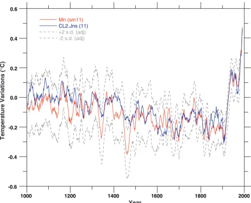
Despite the different number and types of data and different methods of estimating temperatures, comparison of the decadally smoothed variations in each reconstruction (Fig. 1) indicates good agreement (r⫽0.73 for 11-point smoothed correlations over the preanthropogenic interval 1005–1850, with P ⬍0.01). Both records [and the Joneset al. (13) and Briffa (14) reconstructions]

show the “Medieval Warm Period” in the interval ⬃1000 –1300, a transition interval from about 1300 –1580, the 17th-century cold period, the 18th-century recovery, and a cold period in the early 19th century.

Even many of the decadal-scale variations in the Medieval Warm Period are reproduc- ible (12), and both reconstructions [and (13,14)] indicate that peak Northern Hemi- sphere warmth during the Middle Ages was less than or at most comparable to the mid-20th-century warm period (⬃1935–1965).

This result occurs because Medieval temperature peaks were not synchronous in all records (12). The two temperature reconstructions also agree closely in estimating an⬃0.4°C warming between the 17th-century and the mid-20th-century warm period (18).

Volcanic forcing. There is increasing evidence (3, 7–10) that pulses of volcanism significantly contributed to decadal-scale climate variability in the Little Ice Age.

Although some earlier studies (9, 10) of forced climate change back to 1400 used a composite ice core index of volcanism (19), which has a different number of records per unit of time, the present study primarily uses two long ice core records from Crete (20) and the Greenland Ice Sheet Project 2 (GISP2) (21) on Greenland, with a small augmentation from a study of large eruptions recorded in ice cores from both Greenland and Antarctica (22). This approach avoids the potential for biasing model results versus time because of changes in the number of records. Because Southern Hemisphere volcanism north of 20°S influences Northern Hemisphere temperatures, the ice core volcano census samples records down to this latitude. The volcanism record is based on electrical con- ductivity (20) or sulfate measurements (21), and a catalog of volcanic eruptions (23) was used to remove local eruptions (24) and identify possible candidate eruptions in order to weight the forcing accord- ing to latitude. Eruptions of unknown origin were assigned a high-latitude origin unless they also occurred in Antarctic ice

core records (22).

The relative amplitude of volcanic peaks was converted to sulfate concentration by first scaling the peaks to the 1883 Krakatau peak in the ice cores. Although earlier studies (9,10) linearly converted these concentration changes to radiative forcing changes, subse- quent comparison (25) of the very large 1259 eruption [eight times the concentration of sulfate in ice cores from Krakatau and three times the size of the Tambora (1815) eruption (21)] with reconstructed temperatures (11–

14) failed to substantiate a response com- mensurate with a linearly scaled prediction of an enormous perturbation of⬃25 W/m²(26).

Calculations (27) suggest that for stratospheric sulfate loadings greater than about 15 megatons (Mt), increasing the amount of sulfate increases the size of aerosols through coagulation. Because the amount of scattered radiation is proportional to the cross-sectional area, and hence to the 2/3 power of volume (or mass), ice core concentrations estimated as⬎15 Mt were scaled by this amount (25).

Aerosol optical depth was converted to changes in downward shortwave radiative forcing at the tropopause, using the relation- ship discussed in Sato et al.(28). There is significant agreement (29) between the 1000- year-long volcano time series and the concentration-modified Robock and Free (19) times

series (Fig. 2A). Both proxy records show the general trends estimated from ground-based observations of aerosol optical depth (28): the pulse of eruptions in the early 20th century and the nearly 40-year quiescent period of volcanism between about 1920 –1960. Be- cause volcano peaks are more difficult to determine in the expanded firn layer of snow/

ice cores, updated estimates of Northern Hemisphere radiative forcing from Satoet al.

were used to extend proxy time series from 1960 to 1998.

Solar forcing.There has been much discussion about the effect of solar variability on decadal-to-centennial–scale climates (3, 6, 8 –10). An updated version of a reconstruc- tion by Leanet al.(5) that spans the interval 1610 –1998 was used to evaluate this mech- anism [for reference, Free and Robock (10) obtained comparable solar-temperature correlations for the interval 1700 –1980 using the Leanet al. and alternate Hoyt and Schatten (4) solar reconstructions]. The Lean et al.

time series has been extended to 1000 by splicing in different estimates of solar variability based on cosmogenic isotopes. These estimates were derived from ice core measurements (30) of ¹⁰Be, residual ¹⁴C from tree ring records (31), and an estimate of¹⁴C from¹⁰Be fluctuations (30). The justification for including the latter index is that neither of

Fig. 1.Comparison of decadally smoothed Northern Hemisphere mean annual temperature records for the past millennium (1000–1993), based on reconstructions of Mannet al.(Mn) (11) and CL (12). The latter record has been spliced into the 11-point smoothed instrumental record (16) in the interval in which they overlap. CL2 refers to a new splice that gives a slightly better fit than the original (12). The autocorrelation of the raw Mannet al.time series has been used to adjust (adj) the standard deviation units for the reduction in variance on decadal scales.

(3)

the first two splices yields a Medieval solar maximum comparable to that of the present.

Because of concerns about biasing results too much by the latter period, which has much more information than the former, the Bard

14C calculation was included so as to obtain a greater spread of potential solar variations and to allow testing of suggestions (32) that solar irradiance increases could explain the Medieval warming.

Once the splices were obtained, the records were adjusted to yield the potential

⬃0.25% change in solar irradiance on longer time scales (33). Because two of the solar proxies indicate that minimum solar activity occurred in the 14th century, the 0.25% range was set from that time to the present rather than from the 17th century, as was done by Leanet al.[the adjustment is very small for the different solar indices in the 14th century (⬃0.05 W/m²)]. The 20th-century increase in estimated net radiative forcing from low-frequency solar variability is about 10 to 30%

greater than estimated from an independent

method (34). An example of one of the splices is illustrated in Fig. 2B, and the three composites (Fig. 2C) show the pattern of potential solar variability changes used in this study.

Anthropogenic forcing. The standard equivalent radiative forcing for CO₂and other well-mixed trace gases (methane, nitrous oxides, and chlorofluorocarbons) is used after 1850 (Fig. 2D). Pre-1850 CO₂ variations, including the small minimum from about 1600 –1800, are from Etheridge et al.(35).

Radiative forcing effects were computed based on updated radiative transfer calculations (36). The well-constrained change in GHG forcing since the middle of the last century is about four times larger than the potential changes in solar variability based on the reconstructions of Lean et al. (5) and Lockwood and Stamper (34).

Tropospheric aerosols consider only the direct forcing effect (that is, no cloud feed- back), whose global level has been estimated as being about – 0.4 W/m² (37), with the Northern-to-Southern–Hemisphere ratio being in the range of 3 to 4 (38). Because there is an approximate offset in the radiative effects of stratospheric and tropospheric ozone (37), and its total net forcing is on the order of⫹0.2 W/m²(37) and is applicable only to the late 20th century, this GHG was not further considered. Other anthropogenic forcing was not included because evaluations by the Intergovernmental Panel for Climate Change (IPCC) (37) indicate that the confidence in these estimates is very low.

Model

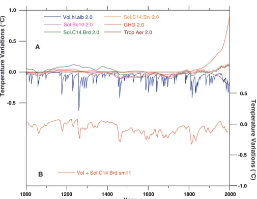
A linear upwelling/diffusion energy balance model (EBM) was used to calculate the mean annual temperature response to estimated forcing changes. This model (39) calculates the temperature of a vertically averaged mixed-layer ocean/atmosphere that is a function of forcing changes and radiative damping. The mixed layer is coupled to the deep ocean with an upwelling/diffusion equation in order to allow for heat storage in the ocean interior. The radiative damping term can be adjusted to embrace the standard range of IPCC sensitivities for a doubling of CO₂. The EBM is similar to that used in many IPCC assessments (40) and has been validated (39) against both the Wigley-Raper EBM (40) and two different coupled ocean-atmosphere general circulation model (GCM) simulations (41). All forcings for the model runs were set to an equilibrium sensitivity of 2°C for a doubling of CO₂. This is on the lower end of the IPCC range (42) of 1.5° to 4.5°C for a doubling of CO₂and is slightly less than the IPCC “best guess” sensitivity of 2.5°C [the inclusion of solar variability in model calculations can decrease the best fit sensitivity (9)]. For both the solar and volcanism runs, Fig. 2.Forcing time series used in the model runs (note scale changes for different panels). (A) (Red)

Ice core millennial volcanism time series from this study (multiplied by –1 for display purposes);

(blue) ice-core Robock and Free (19) reconstruction from 1400 to the present after adjustments discussed in (9) and (25); and (green) Sato et al.(28) Northern Hemisphere radiative forcing, updated to 1998 and multiplied by⫺1 for display purposes. (B) Example of splice for solar variability reconstructions, using the¹⁰Be-based irradiance reconstruction of (30) (red) and the reconstruction of solar variability from Leanet al.(5) (blue). (C) Comparison of three different reconstructions of solar variability based on¹⁰Be measurements (30) (blue),¹⁴C residuals (31) (red), and calculated

14C changes based on ¹⁰Be variations (30) (green). (D) Splice of CO₂radiative forcing changes 1000–1850 (35) (red) and post-1850 anthropogenic changes in equivalent GHG forcing and tropospheric aerosols (blue).

(4)

the calculated temperature response is based on net radiative forcing after adjusting for the 30% albedo of the Earth-atmosphere system over visible wavelengths.

Results

The modeled responses to individual forcing terms (Fig. 3A) indicate that the post-1850 GHG and tropospheric aerosol changes are similar to those discussed in IPCC (42).CO₂ temperature variations are very small for the preanthropogenic interval, although there is a 0.05°C decrease in the 17th and 18th centuries that reflects the CO₂decrease of⬃6 parts per million in the original ice core record (35). Solar variations are on the order of 0.2°C, and volcanism causes large cooling (43) in the Little Ice Age (3–7,9,10). Aver- aged over the entire preanthropogenic interval (Table 1), 22 to 23% of the decadal-scale variance can be explained by volcanism (P⬍ 0.01). However, over the interval 1400 –1850, the volcanic contribution increases to 41 to 49% (P ⬍ 0.01), thereby indicating a very important role for volcanism during the Little Ice Age.

The sun-climate correlations for the interval 1000 –1850 vary substantially by choice of solar index (Table 1), with explained variance ranging from as low as 9% (P⬍0.01) for the¹⁴C residual index (31) to as high as 45% (P⬍0.01) for the Bardet al.(30)¹⁴C solar index, which reconstructs a Medieval solar warming comparable to the present century but only about 0.1°C greater than predicted by the other solar indices (Fig. 3A).

The large range in correlations for the solar records emphasizes the need to determine more precisely the relative magnitude of the real Medieval solar warming peak.

The joint effects of solar variability and volcanism (Fig. 3B) indicate that the combination of these effects could have contributed

0.15° to 0.2°C to the temperature increase (Fig. 1) from about 1905–1955, but only about one-quarter to the total 20th-century

warming. The combined warmth produced by solar variability and volcanism in the 1950s is similar in magnitude but shorter in duration

Fig. 3.(A) Model response to different forcings, calculated at a sensitivity of 2.0°C for a doubling of CO₂. (B) Example of the combined effect of volcanism and solar variability (with 11-point smoothing), using the Bardet al.(30)¹⁴C index.

Fig. 4.Comparison of model response (blue) using all forcing terms (with a sensitivity of 2.0°C) against (A) the CL (12) data set spliced into the 11-point smoothed Joneset al.(16) Northern Hemisphere instrumental record, with rescaling as discussed in the text and in the Fig. 1 caption;

and (B) the smoothed Mannet al. (11) reconstruction. Both panels include the Jones et al.

instrumental record for reference. To illustrate variations in the modeled response, the ¹⁴C calculation from Bardet al.(30) has been used in (A) and the¹⁰Be estimates from (30) have been used in (B).

Table 1. Correlations of volcanism (volc.) and solar variability (sol.) for the preanthropogenic interval, with percent variance shown in parentheses. The different solar time series reflect the three different solar indices used in this study. The Mann et al.time series (11) has been smoothed with an 11-point filter. CL was smoothed in the original analysis (12). Different abbreviations for solar forcing refer to the different indices discussed in the text:¹⁰Be and¹⁴C calculations are from Bard et al. (30);¹⁴C residuals are from Stuiveret al.

(31).

Volc. vs. Mannet al. (1000–1850) 0.48 (23%) Volc. vs. CL (1000–1850) 0.47 (22%) Volc. vs. Mannet al. (1400–1850) 0.70 (49%) Volc. vs. CL (1400–1850) 0.64 (41%) Sol (¹⁰Be) vs. Mannet al. 0.45 (20%) Sol (¹⁴C Bard) vs. Mannet al. 0.56 (31%) Sol (¹⁴C Stuiver) vs. Mannet al. 0.37 (14%) Sol (¹⁰Be) vs. CL 0.42 (18%) Sol (¹⁴C Bard) vs. CL 0.67 (45%) Sol (¹⁴C Stuiver) vs. CL 0.30 ( 9%)

(5)

than the warmth simulated by these mechanisms in the Middle Ages. The variations in the past few decades resulting from the com-

bination of solar variability and volcanism is 0.2°C less than the 1955 peak.

Combining all forcing (solar, volcanism,

GHG, and tropospheric aerosols) results in some striking correspondences between the model and the data over the preanthropogenic interval (Fig. 4). Eleven-point smoothed correlations (44) for the preanthropogenic interval (Table 2) indicate that 41 to 64% of the total variance is forced (P⬍0.01). The high- est correlations are obtained for the CL time series, which has slightly more Medieval warmth than the Mannet al.reconstruction, and for the forcing time series that includes the largest solar estimate of Medieval warmth. Forced variability explains 41 to 59% of the variance (P ⬍ 0.01) over the entire length of the records. Although simulated temperatures agree with observations in the late 20th century, simulations exceed observations by⬃0.1° to 0.15°C over the intervals 1850 –1885 and 1925–1975, with a larger discrepancy between ⬃1885–1925 that reaches a maximum offset of ⬃0.3°C from

⬃1900 –1920. However, decadal-scale pat- terns of warming and cooling are still simulated well in these offset intervals. A sensitivity test (45) comparing forcing time series with and without solar variability indicates that changes caused by volcanism and CO₂ are responsible for the simulated temperature increase from the mid- to late 19th century to the early 20th century, thereby eliminating uncertainties in solar forcing as the explanation for the temperature differences between the model and the data. Also shown in Fig.

4A is the CL reconstruction with the “anom- alous” warm interval (⬃1885–1925) discussed above. For this reconstruction, 55 to 69% of the variance from 1005–1993 can be explained by the model (P⬍0.01).

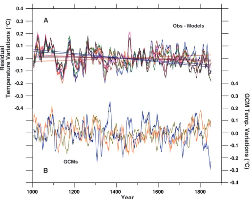
Another means of evaluating the role of forced variability is to determine residuals by subtracting the different model time series from the two paleo time series over the preanthropogenic interval (Fig. 5A). The trend lines for three of these residuals are virtually zero, and there is only about a⫾0.1°C trend for the other three residuals. Because the pre-1850 residuals represent an estimate of the unforced variability in the climate system, it is of interest to compare the smoothed residuals with smoothed estimates of unforced variability in the climate system from control runs of coupled ocean-atmosphere models. There is significant agreement (Fig.

5B and Table 3) between the smoothed standard deviations of the GCMs (46) and paleo residuals (47). These results support a basic assumption in optimal detection studies (1) and previous conclusions (48) that the late- 20th-century warming cannot be explained by unforced variability in the ocean-atmosphere system. However, a combination of GHG, natural forcing, and ocean-atmosphere variability could have contributed to the 1930 –1960 warm period (1,9,10,49).

One way to highlight the unusual nature Fig. 5.Analysis of preanthropogenic residuals in the paleo records. (A) Estimates of residuals using

all combinations of temperature reconstructions and total forcing (including three different solar indices), with trend lines fitted for each of the six residuals. (B) Control runs (detrended) from three different coupled ocean-atmosphere models (46): the NOAA/GFDL model (NOAA Geophysical Fluid Dynamics Laboratory) (orange), the HadCM3 model (Hadley Centre at the UK Meteorological Office, Bracknell, UK) (blue), and the ECHAM3/LSG model (European Centre/University of Ham- burg/Max Planck Institute fu¨r Meteorologie) (brown). For the sake of comparison with the paleo data, the GCM runs have been truncated to the same length as the paleo residuals and have been plotted using the arbitrary starting year of 1000.

Table 2.Correlations between model runs with combined forcing and the Mannet al. (11) and CL (12) time series. Correlations have been subdivided into the following three categories: Top set: Correlations for all the preanthropogenic interval 1005–1850 of model response to combined forcing (“All”) with different solar indices (Table 1) and the 11-point smoothed Mannet al. time series and CL2 record spliced into the 11-point smoothed Joneset al. (16) time series. Middle set: Correlations over the entire interval analyzed. Bottom set: Correlations and variance explained for the interval 1005–1993 using the original CL2 reconstruction from 1005–1965, with the smoothed Joneset al. (16) record added from 1965–1993.

Summary of pre-1850 correlations, with variance shown in parentheses

All¹⁰Be (solar) vs. Mann (sm11) 0.64 (41%)

All¹⁴C Brd (solar) vs. Mann (sm11) 0.68 (46%)

All¹⁴C Stv (solar) vs. Mann (sm11) 0.65 (42%)

All¹⁰Be (solar) vs. CL2.Jns11 0.69 (48%)

All¹⁴C Brd (solar) vs. CL2.Jns11 0.80 (64%)

All¹⁴C Stv (solar) vs. CL2.Jns11 0.68 (47%)

Summary of correlations for 1005–1993, with variance shown in parentheses

All¹⁰Be (solar) vs. Mann (sm11) 0.68 (46%)

All¹⁴C Brd (solar) vs. Mann (sm11) 0.73 (53%)

All¹⁴C Stv (solar) vs. Mann (sm11) 0.67 (45%)

All¹⁰Be (solar) vs. CL2.Jns11 0.66 (43%)

Summary of correlations for 1005–1993 against unfiltered CL time series, with 11-point smoothed Jones et al. (16) record spliced in from 1965–1993

All¹⁰Be (solar) vs. CL2.Jns 11 0.75 (57%)

(6)

of the late-20th-century warmth is to subtract all forcing other than CO₂(solar, volcanism, and tropospheric aerosols) and examine the late-20th-century residuals within the context of the previous 1000 years (Fig. 6). There is an unprecedented residual warming in the late 20th century that matches the warming predicted by GHG forcing. Projection of the

“Business As Usual” (BAU) scenario into the next century using the same model sensitivity of 2.0°C indicates that, when placed in the perspective of the past 1000 years, the warming will reach truly extraordinary levels (Fig.

6). The temperature estimates for 2100 also exceed the most comprehensive estimates (50) of global temperature change during the last interglacial (⬃120,000 to 130,000 years ago)—the warmest interval in the past 400,000 years.

Discussion

Forcing a linear energy balance model with independently derived time series of volcanism and solar variability indicates that 41 to 64% of the preanthropogenic low-frequency variance in temperature can be accounted for by external factors. These results were obtained without any retuning of the climate model. When the same sensitivity for the preanthropogenic interval is used for the past 150 years, there is good agreement with temperatures in the late 20th century. Some cau- tion is needed in interpreting the agreement between models and data for a 2.0°C sensitivity, because a more detailed analysis of uncertainties (47) might yield slightly different sensitivities than simulated here (51).

Also, statistical methods better constrain the minimum than the maximum sensitivity (52).

If paleo records are shown to have had larger amplitude than used in this study (18), model-data correlations should still be valid but the best fit sensitivity would be greater.

The largest model-data discrepancy over the entire past 1000 years is from ⬃1885–

1925, peaking in ⬃1900 –1920. Although such differences could reflect random uncertainties in the paleo reconstructions (Fig. 1) or forcing fields, the consistent offset between model and data suggests the need to identify one or more specific explanations for the differences. For example, two factors that could be contributing to the model-data differences in this interval are: (i) mid-latitude land clearance may have increased albedo and caused slightly greater cooling than simulated (53), and (ii) warming may be under- estimated in the early stage of the instrumental record because of sparse data coverage (16). As discussed above, there is evidence for warming in some of the high-elevation data in the original CL (12) reconstruction and in the comprehensive Overpecket al.(6) Arctic synthesis. Many alpine glaciers started to retreat around 1850 (54). There is also

some evidence for warming of tropical oceans in the late 19th century (16), but the data are very sparse. More data and model analyses would be required to test these and other possible explanations.

Analysis of residuals in the pre-1850 interval reveals little or no trend. If the pre-

1850 temperature reconstructions, forcing estimates, and model responses are correct, the model-data agreement in this study suggests that factors such as thermohaline circulation changes (55) may have played only a second- ary role with respect to modifying hemispher- ic temperatures over the past 1000 years (56).

Fig. 6.Comparison of the GHG forcing response (from Fig. 3) with six residuals determined by removing all forcing except GHG from the two different temperature reconstructions in Fig. 1. As in Fig. 5, the three different estimates of solar variability were used to get one estimate of the uncertainty in the response. This figure illustrates that GHG changes can explain the 20th-century rise in the residuals; ⫾2 standard deviation lines (horizontal dashed lines) refer to maximum variability of residuals from Fig. 5A (inner dashes) and maximum variability (outer dashes) of the original pre-1850 time series (Fig. 1). The projected 21st-century temperature increase (heavy dashed line at right) uses the IPCC BAU scenario (the “so-called IS92a forcing”) for both GHG and aerosols (sulfate and biomass burning, including indirect effects), and the model simulation was run at the same sensitivity (2.0°C for a doubling of CO₂) as other model simulations in this article. The IS92a scenario is from (59).

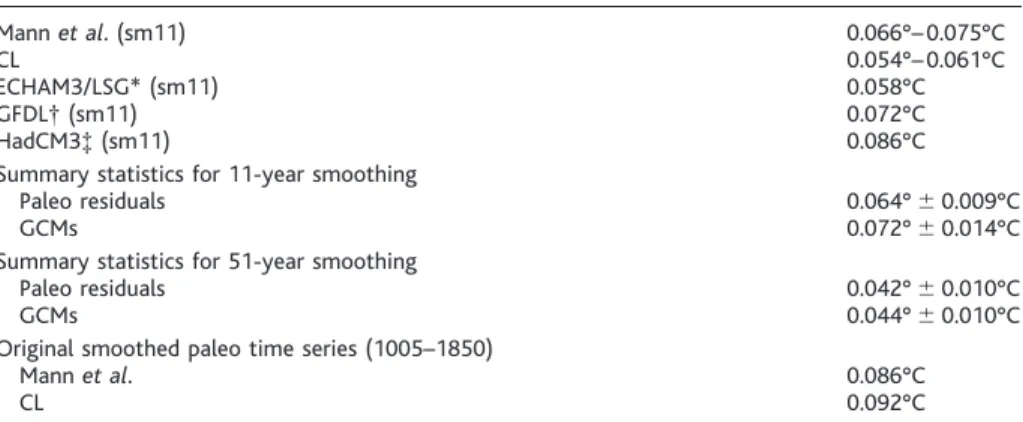
Table 3. Comparison of smoothed standard deviations (in °C) of 850-year Northern Hemisphere preanthropogenic residuals from observations with smoothed 850-year coupled ocean-atmosphere GCM control runs (46). All records were detrended except for the original smoothed paleo time series.

Mannet al. (sm11) 0.066°–0.075°C

CL 0.054°–0.061°C

ECHAM3/LSG* (sm11) 0.058°C

GFDL†(sm11) 0.072°C

HadCM3‡(sm11) 0.086°C

Summary statistics for 11-year smoothing

Paleo residuals 0.064°⫾0.009°C

GCMs 0.072°⫾0.014°C

Summary statistics for 51-year smoothing

Paleo residuals 0.042°⫾0.010°C

GCMs 0.044°⫾0.010°C

Original smoothed paleo time series (1005–1850)

Mannet al. 0.086°C

CL 0.092°C

*The European Centre/University of Hamburg/Max Planck Institute fu¨r Meteorologie model. †The NOAA Geophysi- cal Fluid Dynamics Laboratory model, Princeton, New Jersey. ‡The Hadley Centre model at the UK Meteorological Office, Bracknell, UK.

(7)

Mannet al.(11) suggested that the decrease in summer insolation since the early Holo- cene (57) also could have contributed to the cooling between the Middle Ages and the Little Ice Age. However, calculations (58) do not support this suggestion.

There are therefore two independent lines of evidence pointing to the unusual nature of late-20th-century temperatures. First, the warming over the past century is unprecedented in the past 1000 years. Second, the same climate model that can successfully explain much of the variability in Northern Hemisphere temperature over the interval 1000 –1850 indicates that only about 25% of the 20th-century temperature increase can be attributed to natural variability. The bulk of the 20th-century warming is consistent with that predicted from GHG increases. These twin lines of evidence provide further support for the idea that the greenhouse effect is already here. This assertion may seem sur- prising to some because of continuing uncertainties with respect to the dynamical response of the ocean-atmosphere system and radiative forcing feedbacks (both direct and indirect) of, for example, clouds, biomass burning, and mineral dust. Although regional climate change is almost certainly influenced by these complex dynamic and thermody- namic feedbacks, the striking agreement seen in this study between simple model calculations and observations indicates that on the largest scale, temperature responds almost linearly to the estimated changes in radiative forcing. The very good agreement between models and data in the preanthropogenic interval also enhances confidence in the overall ability of climate models to simulate temperature variability on the largest scales.

References and Notes

1. B. D. Santeret al., Nature382, 39 (1996); G. C.

Hegerlet al.,Clim. Dyn.13, 613 (1997); G. R. North and M. J. Stevens,J. Clim.11, 563 (1998); S. F. B. Tett et al.,Nature399, 569 (1999); T. P. Barnettet al., Bull. Am. Meteorol. Soc. 80, 2631 (1999); G. C.

Hegerlet al.,Clim. Dyn., in press.

2. T. P. Barnett, B. D. Santer, P. D. Jones, R. S. Bradley, K. R. Briffa,Holocene6, 255 (1996).

3. A. Robock,Science206, 1402 (1979); T. M. L. Wigley and S. C. B. Raper,Nature344, 324 (1990); P. M. Kelly and T. M. L. Wigley, Nature360, 328 (1992); E.

Friis-Christensen and K. Lassen, Science254, 698 (1991); T. J. Crowley and K.-Y. Kim,Quat. Sci. Rev.12, 375 (1993); D. Rind and J. Overpeck,Quat. Sci. Rev.

12, 357 (1993); U. Cubaschet al.,Clim. Dyn.13, 757 (1997); P. E. Damon and A. N. Peristykh,Geophys.

Res. Lett.26, 2469 (1999); J. Lean and D. Rind,J.

Atmos. Sol. Terr. Phys.61, 25 (1999).

4. D. V. Hoyt and K. H. Schatten,J. Geophys. Res.98, 18895 (1993).

5. J. Lean, J. Beer, R. Bradley, Geophys. Res. Lett.22, 3195 (1995).

6. J. Overpecket al.,Science278, 1251 (1997).

7. K. R. Briffa, P. D. Jones, F. H. Schweingruber, T. J.

Osborn,Nature393, 450 (1998).

8. M. E. Mann, R. S. Bradley, M. R. Hughes,Nature392, 779 (1998).

9. T. J. Crowley and K.-Y. Kim,Geophys. Res. Lett.26, 1901 (1999).

10. M. Free and A. Robock,J. Geophys. Res.104, 19057 (1999).

11. M. E. Mann, R. S. Bradley, M. K. Hughes,Geophys. Res.

Lett.26, 759 (1999).

12. T. J. Crowley and T. S. Lowery,Ambio29, 51 (2000).

13. P. D. Joneset al.,Holocene8, 467 (1998).

14. K. R. Briffa,Quat. Sci. Rev.19, 87 (2000).

15. Although it is well known that many proxy climate indices are strongly influenced by seasonal variations, such variations map into and influence mean annual temperatures [T. J. Crowley and K.-Y. Kim,Geophys.

Res. Lett.23, 359 (1996); G. C. Jacoby and R. D.

D’Arrigo,Geophys. Res. Lett.23, 2197 (1996); T. J.

Crowley and K.-Y. Kim,Geophys. Res. Lett.23, 2199 (1996)].

16. P. D. Jones, M. New, D. E. Parker, S. Martin, I. G. Rigor, Rev. Geophys.37, 173 (1999).

17. D. A. Graybill and S. B. Idso, Global Biogeochem.

Cycles7, 81 (1993).

18. Although borehole estimates of temperature change over the past few centuries are greater in magnitude than surface proxy data [S. Huanget al.,Nature403, 756 (2000)], there are concerns about the potential effects of changes in land use on borehole records [W. R. Skinner and J. A. Majorowicz,Clim. Res.12, 39 (1999)]. (See the “Discussion” section of this paper for further comments on this issue.)

19. A. Robock and M. P. Free, inClimatic Variations and Forcing Mechanisms of the Last 2000 Years, R. S.

Bradley, P. D. Jones, J. Jouzel, Eds. (Springer-Verlag, Berlin, 1996), pp. 533–546.

20. C. U. Hammer, H. B. Clausen, W. Dansgaard,Nature 288, 230 (1980); T. J. Crowley, T. A. Christe, N. R.

Smith,Geophys. Res. Lett.20, 209 (1993).

21. G. A. Zielinski,J. Geophys. Res.100, 20937 (1995).

22. C. C. Langway Jr., K. Osada, H. B. Clausen, C. U.

Hammer, H. Shoji, J. Geophys. Res. 100, 16241 (1995).

23. T. Simkin and L. Siebert, Volcanoes of the World (Geoscience Press, Tucson, AZ, ed. 2, 1994).

24. An exception is the June 1783–January 1784 Laki (Iceland) eruption, which had an estimated Northern Hemisphere sulphur loading comparable to the combined effect of the three Caribbean eruptions in 1902 (21). Although this eruption primarily increased the tropospheric aerosol loading, the persistence and magnitude of the eruption may have approached anthropogenic troposphere sulfur emission values and had a discernible influence on Northern Hemi- sphere temperatures [C. Hammer,Nature270, 482 (1977); H. Sigurdsson,Eos63, 601; (7); G. J. Jacoby, K. W. Workman, R. D. D’Arrigo,Quat. Sci. Rev.18, 1365 (1999)].

25. W. T. Hyde and T. J. Crowley, J. Clim.13, 1445 (2000).

26. An informal survey of published historical records also failed to yield any clear evidence for extremely severe agricultural disruptions at this time (as would be expected if linear scaling of the ice core sulphate concentration applies). The study by Langwayet al.

(22) clearly indicates that evidence of this eruption occurs in both Greenland and Antarctic ice cores.

27. J. P. Pinto, R. P. Turco, O. B. Toon,J. Geophys. Res.94, 11165 (1989).

28. M. Sato, J. E. Hansen, M. P. McCormick, J. B. Pollack,J.

Geophys. Res.98, 22987 (1993).

29. Because of the noisy nature of the volcanic series, EBM runs were used to correlate the two long volcano time series illustrated in Fig. 2A. The 11-point smoothed correlation for the interval 1405–1960 is 0.78 (P⬍0.01).

30. Beryllium-10 measurements are from E. Bardet al., Earth Planet. Sci. Lett.150, 453 (1997); the irradiance estimates derived from the¹⁰Be measurements are from E. Bardet al.,Tellus B52, 985 (2000).

31. M. Stuiver and T. F. Braziunas,Radiocarbon35, 137 (1993).

32. G. H. Denton and W. Karle´n,Quat. Res.3, 155 (1973).

33. J. Lean, A. Skumanich, O. White,Geophys. Res. Lett.

19, 1591 (1992).

34. M. Lockwood and R. Stamper,Geophys. Res. Lett.26, 2461 (1999).

35. D. M. Etheridgeet al.,J. Geophys. Res.101, 4115 (1996).

36. G. Myhre, E. J. Highwood, K. P. Shine, F. Stordal, Geophys. Res. Lett.25, 2715 (1998).

37. D. Schimel et al., in Climate Change 1995, J. T.

Houghtonet al., Eds. (Cambridge Univ. Press, Cam- bridge, 1996), pp. 65–132.

38. J. M. Haywood and V. Ramaswamy,J. Geophys. Res.

103, 6043 (1998); J. E. Penner, C. C. Chuang, K. Grant, Clim. Dyn.14, 839 (1998); J. T. Kiehl, T. L. Schneider, P. J. Rasch, M. C. Barth, J. Wong,J. Geophys. Res.105, 1441 (2000).

39. K.-Y. Kim and T. J. Crowley,Geophys. Res. Lett.21, 681 (1994).

40. T. M. L. Wigley and S. C. B. Raper,Nature330, 127 (1987).

41. U. Cubaschet al.,Clim. Dyn.8, 55 (1992); S. Manabe and R. J. Stouffer,Nature363, 215 (1993).

42. A. Kattenberget al., inClimate Change 1995, J. T.

Houghtonet al., Eds. (Cambridge Univ. Press, Cam- bridge, 1996), pp. 285–358.

43. Although the effects of volcanism are primarily man- ifested in the summer hemisphere, these changes map into mean annual temperature variations at a reduced level, and the EBM is tuned to simulate mean annual temperatures. The reliability of this approach is supported by good agreement between the EBM and recent GCM studies (P. Stottet al.,Clim. Dyn., in press) of a decadally averaged cooling effect from volcanism during the late 20th century. The EBM predicts a 0.2°C cooling; the GCM predicts a 0.3°C cooling. Given the facts that the ensemble GCM run has noise in it and that the GCM has a sensitivity greater than the EBM, the EBM-GCM results are not considered to be significantly different.

44. An alternate approach using 8-point smoothing fol- lowed by 5-point smoothing yields virtually identical correlations (such sequential smoothing can substantially improve the filter characteristics of a running average).

45. T. J. Crowley, data not shown.

46. S. Manabe and R. J. Stouffer,J. Clim.9, 376 (1996); R.

Voss, R. Sausen, U. Cubasch,Clim. Dyn.14, 249 (1998); M. Collins, S. F. B. Tett, C. Cooper,Clim. Dyn., in press.

47. There are a number of uncertainties with respect to the estimate of unforced variability from proxy data.

Because proxy reconstructions do not correlate per- fectly with temperature, proxy variance may differ from the true variance. Also, residuals may include some component of forced variability due to errors in the forcing or temperature reconstructions. If multi- regression is used to best fit the model to observations, the residuals will also differ slightly.

48. R. J. Stouffer, S. Manabe, K. Y. Vinnikov,Nature367, 634; R. J. Stouffer, G. Hegerl, S. Tett,J. Clim.13, 513 (2000).

49. T. L. Delworth and T. R. Knutson,Science287, 2246 (2000); T. L. Delworth and M. E. Mann,Clim. Dyn., in press.

50. Despite clear evidence for seasonal and regional temperature changes greater than the present during the last interglacial (120,000 to 130,000 years ago), there are few quantitative estimates of global temperature change for this time. The most comprehensive assessment is based on an analysis of sea surface temperature (SST) variations [W. F. Ruddiman and CLIMAP Members,Quat. Res.21, 123 (1984)], which indicate an average SST for the last interglacial within 0.1°C of the mid-20th-century calibration period.

This result agrees closely with that produced from a coupled ocean-atmosphere simulation [M. Montoya, T. J. Crowley, H. von Storch,Paleoceanography13, 170 (1998)]. The same model yields global temperatures only 0.3°C warmer than the control run [M.

Montoya, H. von Storch, T. J. Crowley,J. Clim.13, 1057 (2000)]. The reason why regional temperatures greater than at present during the last interglacial do not translate into a large global temperature difference is because winter cooling offsets summer warming in some time series and because there are significant phase offsets between the timing of peak warmth in different regions [T. J. Crowley,J. Clim.3, 1282 (1990)].

51. Preliminary results suggest that a 2.0°C sensitivity slightly overestimates the response (G. C. Hegerl and T. J. Crowley, in preparation), but it is not yet clear