M.Sc., Carleton University, Ottawa, Ontario, 2010

Measurement of the Top Quark Mass in the All-Hadronic Top-Antitop Decay Channel Using Proton-Proton Collision Data from the ATLAS Experiment at a Centre-of-Mass Energy of 8 TeV

by

Thomas G. McCarthy

B.Sc. Honours, Trent University, Peterborough, Ontario, 2005 B.Ed., Queen’s University, Kingston, Ontario, 2006

M.Sc., Carleton University, Ottawa, Ontario, 2010

A thesis submitted to the

Faculty of Graduate and Post Doctoral Affairs in partial fulfillment of the requirements for the degree of

Doctor of Science

Ottawa-Carleton Institute for Physics Department of Physics

Carleton University Ottawa, Ontario, Canada

September, 2015

copyright c

Thomas G. McCarthy, 2015

Abstract

A measurement of the top quark mass (m

) is presented using top quark candidates re- constructed from the jets in all-hadronic t ¯ t decays. The analysis makes use of the full ATLAS dataset collected over the 2012 period at a centre-of-mass energy of √

s = 8 TeV and with a total integrated luminosity of R

Ldt = 20.6 fb

. A five-jet trigger, together with an offline cut requiring five central jets with a transverse momentum of at least 60 GeV, was used to pre- select candidate signal events. A series of selection cuts are subsequently employed to increase the signal fraction in data events, motivated by both measured data and simulation. These cuts, as well the analytic χ

reconstruction algorithm to designate which jets are to be used to reconstruct the top quarks, aim to select those events and candidate top quarks deemed most consistent with an all-hadronic t ¯ t decay topology. The most discriminating cut involves the output of a b-tagging algorithm employed to identify jets suspected as having been initiated by a bottom-type quark – a key signature of top quark decays.

The measurement is made using a one-dimensional template method, in which a series of distributions are produced for an observable sensitive to the top quark mass by using simulated signal samples with varying input m

values. The ratio of the three- to two-jet invariant masses of candidate top quark - W boson pairs is selected as the m

-sensitive observable, as it is less susceptible to uncertainties arising from the jet energy scale, thereby reducing the corresponding systematic uncertainty on m

. The contributions from backgrounds, including the dominant QCD multi-jet production but also t ¯ t events with at least one leptonic W boson decay, are estimated using a mix of simulation and data-driven methods.

The final measurement is made via a binned χ

minimization procedure which takes into account uncertainties in the bin contents from the measured data as well as uncertainties in the parameterization for both signal and background shapes.

The final measured value is found to be m

= 174.29 ± 0.52 (stat) ± 1.03 (syst) GeV, consistent both with recent LHC measurements in the same and orthogonal decay channels and the current world average. The fraction of background events within the range of the final distribution, measured simultaneously, is found to be F

= 0.517 ± 0.015 (stat)±0.075 (syst).

ii

Acknowledgements

Many thanks to my supervisor Gerald Oakham for his patience, his absolute trust, and his unwavering support throughout my years at Carleton. You were the calm and steady voice of reason, and were always there when I needed you. Whenever I had any doubts, I knew I could count on you to support me 100% of the time. Thank you.

A great deal of thanks also to the various members of Carleton’s ATLAS group present throughout my M.Sc. and Ph.D. programs for all the feedback and fruitful discussions. In particular I wish to thank Manuella Vincter for her support in promoting outreach work, and Alain Bellerive for sharing his expertise in statistics. To the ATLAS graduate students who have been with me over the years, thanks for the many chats, the coffee breaks, and of course the arguments we got into over assignments earlier in our program – likely where we learned the most.

To Teresa Barillari, Sven Menke, Andi Wildauer and the members of the HEC group at the Max Planck Institute for Physics in Munich: my year in Germany was certainly a defining time for me, and working with your group and the time I spent in Bavaria marked the highlight of my program. I can’t thank you enough for everything. A particular thank you to Gerald, to Sven and to Teresa for providing me with this opportunity.

Thanks also to my family: to my parents Richard and Marilyn for always supporting me in whatever decision I made, whether personal or professional, and to my siblings Brian, Matthew

& Kathy. I really appreciate you all being there for me since I started my M.Sc. program.

I would also like to acknowledge the generous support of the Natural Sciences and Engineering Research Council of Canada.

iii

Contents

Abstract ii

Acknowledgments iii

Table of Contents iv

List of Tables x

List of Figures xi

Glossary of Terms xv

1 Introduction 1

2 Theoretical Background 3

2.1 The Standard Model of Particle Physics . . . . 3

2.2 The Top Quark . . . . 5

2.2.1 Role in the Standard Model . . . . 5

2.2.2 Production Mechanisms . . . . 5

2.2.3 The Partonic Structure of the Proton . . . . 7

2.2.4 Decay Modes . . . . 14

2.2.5 Properties . . . . 18

2.2.6 Mass . . . . 19

3 The ATLAS Experiment 22 3.1 CERN and the Large Hadron Collider . . . . 22

iv

3.2 The ATLAS Detector . . . . 22

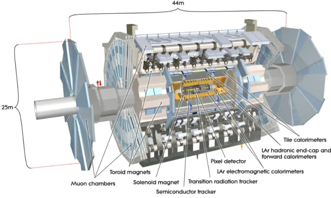
3.2.1 Coordinate System and Useful Collider Physics Formulae . . . . 23

3.2.2 Interaction of Particles with Matter . . . . 26

3.2.3 Overview of the Various Detector Components . . . . 27

3.2.4 Inner Detector . . . . 27

3.2.5 Electromagnetic and Hadronic Calorimeters . . . . 28

3.2.6 Muon Spectrometer . . . . 32

3.2.7 Particle Signatures in ATLAS . . . . 32

3.2.8 High-Level Trigger System . . . . 34

3.2.9 ATLAS 2012 Dataset . . . . 34

4 Quarks & Jets 36 4.1 Quark Signatures in ATLAS . . . . 36

4.2 The Anti-k

Jet Reconstruction Algorithm . . . . 37

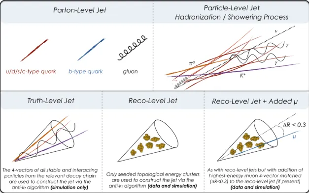
4.3 Levels of Jet Reconstruction . . . . 38

4.4 Jet Flavour and Tagging . . . . 42

4.4.1 Jet Flavour . . . . 42

4.4.2 b-Tagging Efficiencies and Rejection Rates . . . . 45

4.5 Jet Energy Response and Resolution . . . . 48

4.5.1 Jet Energy Response Relative to Quarks . . . . 48

4.5.2 Jet Energy Response Relative to Truth Jets . . . . 49

4.5.3 Semileptonic Quark Decays and Matched Muons . . . . 52

4.6 Standard Corrections to Reconstructed Jets . . . . 54

4.6.1 Area and Offset Corrections Due to Pile-Up Activity . . . . 54

4.6.2 Origin Correction . . . . 55

4.6.3 Absolute Jet Energy Scale (JES) Correction . . . . 55

4.6.4 Global Sequential Calibration . . . . 56

4.6.5 Residual In-Situ Correction . . . . 56

4.6.6 Summary of Jet Corrections . . . . 56

5 All-Hadronic t t ¯ Signal and Associated Background Processes 57 5.1 All-Hadronic t t ¯ Signal Processes . . . . 57

v

5.1.1 Simulated Monte Carlo Datasets . . . . 57

5.1.2 Kinematics of All-Hadronic t t ¯ Events . . . . 59

5.2 Background Processes . . . . 64

5.2.1 QCD Multi-Jet Production . . . . 64

5.2.2 Non All-Hadronic t ¯ t . . . . 65

5.2.3 Combinatorial Background from Signal Events . . . . 65

6 Top Quark Reconstruction 67 6.1 Jet-Quark Assignment in Reconstruction Algorithms . . . . 67

6.2 Levels of Top Quark Reconstruction . . . . 70

6.3 Reconstruction Purity in Simulated Signal Events . . . . 72

6.4 Event Reconstruction Using a χ

Minimization . . . . 74

6.4.1 Reconstruction χ

Definition . . . . 75

6.4.2 Detector Response and Resolution Reference Terms . . . . 77

6.4.3 Reconstruction Goodness of Fit Probability (P

) . . . . 79

6.5 Performance of χ

Reconstruction on Signal Events . . . . 79

6.6 Summary of Top Quark Decay and Reconstruction . . . . 82

7 Event Selection 83 7.1 Introduction . . . . 83

7.2 Object Definitions . . . . 85

7.2.1 Jets . . . . 85

7.2.2 Leptons (e/µ) . . . . 86

7.2.3 Missing Transverse Energy (E

) . . . . 87

7.3 Summary of Full Event Selection . . . . 88

7.4 Descriptions of Event Selection Cuts . . . . 92

7.4.1 Motivation Using Normalized Shape Comparisons . . . . 92

7.4.2 Pre-Selection (C1) . . . . 94

7.4.3 Trigger and Offline p

Requirement (C2) . . . . 94

7.4.4 Jet Isolation (C3) . . . . 95

7.4.5 Six Central Jet Requirement (C4) . . . . 96

7.4.6 Five Central Jet and Offline p

Requirement (C5) . . . . 96

vi

7.4.7 Missing Transverse Energy (C6) . . . . 96

7.4.8 Gluon Splitting (g → b ¯ b) Suppression (C7) . . . . 97

7.4.9 Top Reconstruction Goodness of Fit (C8) . . . . 97

7.4.10 Number of Tagged Jets (C9) . . . . 98

7.4.11 Angular Separations of Reconstructed Objects (C10) . . . . 98

8 Signal Templates of the R

Observable 100 8.1 Template Method Overview . . . 100

8.2 R

as the Top Quark Mass-Sensitive Observable . . . 101

8.3 Parameterization of R

Signal Template Shapes . . . 104

8.4 Extracted Signal Template Parameters . . . 108

8.4.1 Extracted Parameters from Individual Fits . . . 108

8.4.2 Extracted Parameters from a Global Fit . . . 111

8.5 Summary of Constructed Signal Templates . . . 112

9 Background Modelling Using the ABCD Method 113 9.1 QCD Multi-jet Background Estimation . . . 113

9.2 Control Plots of Event Kinematic Variables . . . 120

9.2.1 Agreement in Control Plots . . . 121

9.3 Estimated QCD Background for the R

Observable . . . 128

9.4 Use of the Estimated QCD Multi-Jet Background . . . 131

10 Top Quark Mass Determination 132 10.1 χ

Minimization and Linear Algebra Framework . . . 132

10.2 Propagation of R

Shape Uncertainties . . . 134

10.2.1 Correlations in Signal and Background Shape Parameters . . . 135

10.3 Extracting the Measured Top Quark Mass . . . 140

10.3.1 Accounting for Correlation Between R

Values . . . 141

10.3.2 Extracted Values of m

and F

. . . 142

11 Sources of Systematic Uncertainty 143 11.1 Introduction . . . 143

11.2 Template Method Closure . . . 145

vii

11.3 Statistical Component of Systematic Uncertainties . . . 153

11.4 Optimization of Event Selection Cuts . . . 154

11.5 Theory- and Modelling-Related Uncertainties . . . 154

11.5.1 Monte Carlo Generator . . . 154

11.5.2 Hadronization Modelling . . . 155

11.5.3 Proton Parton Distribution Functions . . . 155

11.5.4 Initial and Final State Radiation . . . 156

11.5.5 Underlying Event . . . 156

11.5.6 Colour Reconnection . . . 156

11.6 Method-Dependent Uncertainties . . . 157

11.6.1 Non-Closure of Template Method . . . 157

11.6.2 Signal and Background Parameterization . . . 157

11.6.3 Inclusion of Non All-Hadronic t ¯ t Background . . . 157

11.6.4 Variation in the Number of Control Regions . . . 159

11.7 Calibration- and Detector-Related Uncertainties . . . 162

11.7.1 Trigger Efficiency . . . 162

11.7.2 Fast vs. Full-Simulation for Monte Carlo Signal Samples . . . 164

11.7.3 Pile-up Reweighting Scale . . . 165

11.7.4 Dependence on Pile-Up Activity . . . 165

11.7.5 Lepton and E

Soft Term Calibrations . . . 166

11.7.6 b-Tagging Scale Factors . . . 167

11.7.7 Jet Energy Scale (JES) . . . 167

11.7.8 b-Jet Energy Scale (bJES) . . . 169

11.7.9 Jet Energy Resolution . . . 169

11.7.10 Jet Reconstruction Efficiency . . . 169

12 Results & Conclusions 171 12.1 Potential for Improved Precision . . . 172

12.2 Future Top Quark Mass Measurements . . . 176

A Personal Contributions to the Analysis 178

viii

B Summary of Simulated Datasets and Monte Carlo Event Weights 181

B.1 Monte Carlo Samples . . . 181

B.2 Monte Carlo Event Weights . . . 182

B.3 Normalization of Simulated Distributions . . . 186

C Additional Analysis Plots and Studies 187 C.1 Signal Shape Jacobian Transformation Matrices . . . 187

C.2 Additional Template Method Closure Plots . . . 189

C.3 Drawing Pseudo Events from 2D Distributions . . . 192

C.4 Correction to the Statistical Uncertainty . . . 195

C.5 Top Reconstruction Performance . . . 197

C.6 Normalized R

Shape Comparisons . . . 201

C.7 Comparison of b-Tagging Working Points . . . 201

D Additional Jet Energy Response and Resolution Plots 202 D.1 Energy Response Relative to Quarks . . . 204

D.2 Energy Response of b-Flavoured Jets . . . 205

D.3 Energy Response Relative to Truth Jets . . . 207

D.4 Flavour Fractions and Average Response . . . 208

E Parton-Level Jet Energy Correction 209 E.1 Theoretical Motivation . . . 210

E.2 Derived Corrections from Simulated Signal Events . . . 214

References 220

ix

List of Tables

2.1 Branching ratios of the three dominant t ¯ t decay channels . . . . 15 4.1 Jet-quark matching and b-tag efficiencies in simulated signal events . . . . 47 4.2 Fraction of reconstructed jets with matched muons by flavour . . . . 54 6.1 Numbers of possible jet-quark permutations for varying jet multiplicities . . . . 69 7.1 Event yields for each sequential event selection cut . . . . 89 8.1 Extracted signal shape template parameters for both individual and global fits . 112 9.1 Estimated signal fractions in each of the four ABCD control and signal regions . 116 9.2 Overall data vs. estimation summary in final signal region D . . . 129 9.3 Extracted R

template parameter values for the QCD multi-jet background . . 131 11.1 Summary of sources of statistical and systematic uncertainties on m

and F

144 11.2 Relevant values for oversampling corrections for the template closure tests . . . 150 11.3 Breakdown of contributions to the JES systematic uncertainty . . . 168 11.4 Breakdown of the bJES, b-tagging, and lepton/E

systematic uncertainties . . 170 12.1 Expected gains in performance with a b-tagging requirement . . . 175 B.1 Summary of all simulated Monte Carlo samples used in the analysis (I) . . . 183 B.2 Summary of all simulated Monte Carlo samples used in the analysis (II) . . . 184 C.1 Comparison of signal fraction and efficiency for various b-tagging working points 201

x

List of Figures

2.1 Standard Model quarks and leptons . . . . 4

2.2 Standard Model bosons . . . . 4

2.3 Peak instantaneous luminosity values during ATLAS Run I data-taking . . . . . 7

2.4 Sample parton distribution functions and t ¯ t production thresholds . . . . 8

2.5 Standard Model top quark production modes at the LHC . . . . 9

2.6 Measured and theoretical production cross-sections at ATLAS . . . . 11

2.7 Recent LHC and Tevatron t t ¯ production cross section measurements . . . . 13

2.8 Recent ATLAS single top quark production cross section measurements . . . . . 13

2.9 Decay channel categorizations of Standard Model W bosons . . . . 14

2.10 Standard Model single top quark and top-antitop quark pair (t ¯ t) decay modes . 17 2.11 Illustrations of some of the roles played by the top quark . . . . 19

2.12 Recent LHC and Tevatron top quark mass measurements . . . . 20

2.13 Updated top quark mass measurements from LHC experiments . . . . 21

3.1 A cutaway view of the ATLAS detector at CERN’s Large Hadron Collider . . . 23

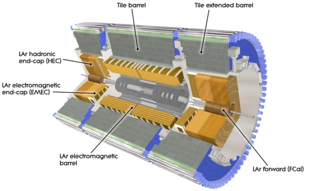
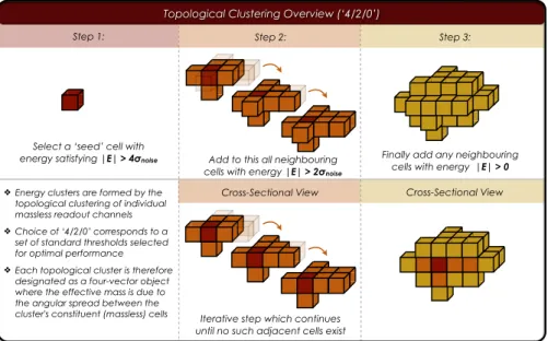
3.2 Relations between the rapidity, pseudorapidity, and the polar angle in ATLAS . 25 3.3 A cutaway view of the ATLAS electromagnetic and hadronic calorimeter system 29 3.4 Illustration of the topological clustering algorithm for readout channels . . . . . 30

3.5 The interactions of various particle types in the ATLAS detector . . . . 33

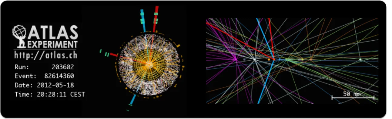
3.6 A candidate ATLAS event display for the process H → ZZ

→ e

e

e

e

. . . . 35

3.7 ATLAS integrated luminosity and average interactions per bunch crossing in 2012 35 4.1 Illustrations of jet reconstruction at various levels . . . . 39

4.2 Illustrations of key jet flavour-tagging variables . . . . 41

xi

4.3 Jet-quark matching efficiency vs. pseudorapidity in simulated signal events . . . 43

4.4 Flavour decomposition of jet energy and pseudorapidity in simulated signal events 44 4.5 Jet b-tagging efficiency as a function of pseudorapidity in simulated signal events 46 4.6 Series of representative plots used to evaluate b-jet energy response and resolution 50 4.7 Jet energy response and resolution for jets of various flavour from signal events . 51 4.8 Jet energy response and fractional resolution based on matches to muons . . . . 53

5.1 Leading-order production diagram for the all-hadronic t ¯ t signal process . . . . . 58

5.2 Sensitivity of truth-level quantities to √ ˆ s and γ

in simulated signal events . . 60

5.3 Sensitivity of truth-level quantities to m

in simulated signal events . . . . 60

5.4 Distributions associated with bottom-type quarks in simulated signal events . . 63

5.5 Leading-order diagrams for the various background processes . . . . 63

6.1 Illustration of top quark reconstruction at various levels . . . . 70

6.2 W boson and top quark invariant mass distributions in simulated signal events . 71 6.3 Illustration of the three reconstruction purity classifications . . . . 73

6.4 Reference mass terms used as inputs to the χ

top reconstruction method . . . . 76

6.5 Reconstruction χ

output for correct-permutation simulated signal events . . . . 78

6.6 Purity decomposition of invariant mass distributions in simulated signal events . 80 6.7 Evolution of Reconstruction: Energy Deposits to Top Quarks . . . . 82

7.1 Depiction of event selection cuts C1 through C10 . . . . 84

7.2 Event yields following each sequential event selection cut . . . . 91

7.3 Pass-through event yields as a function of each omitted event selection cut . . . 91

7.4 Normalized shape comparisons for several key event selection variables . . . . . 93

7.5 Trigger efficiency vs. fifth jet offline p

in simulated signal events . . . . 95

8.1 Sensitivity of the R

observable to m

. . . 102

8.2 Sensitivity of m

and R

to JES in simulated signal events . . . 102

8.3 Parton-level R

distribution in simulated signal events . . . 103

8.4 Reconstruction-level R

distributions in simulated signal events . . . 105

8.5 Results of individual fits to R

distributions for various m

samples . . . 107

8.6 R

signal template Gaussian mean parameter as a function of m

. . . 109

xii

8.7 Remaining R

signal template parameters as a function of the generator m

. 109 8.8 Signal R

distribution for m

= 172.5 GeV together with overlaid global fit . 110 8.9 Results of a global fit to all signal R

distributions for various m

samples . . 110 9.1 Classification of four ABCD regions used in the background estimation method . 115 9.2 Signal contribution in ABCD regions used in the background estimation method 115 9.3 Correlation plots for the data-driven QCD background estimation method. . . . 117 9.4 Control plots showing the p

distributions of the six leading jets . . . 122 9.5 Control plots showing the η distributions of the six leading jets . . . 123 9.6 Control plots showing the φ distributions of the six leading jets . . . 124 9.7 Additional control plots of two- and three-jet invariant mass distributions . . . . 126 9.8 Additional control plots of jet multiplicity and reconstruction χ

and P

. . 127 9.9 Estimated R

shapes for the QCD multi-jet background in each ABCD region 130 9.10 Final data and estimation comparison plot for the R

observable . . . 130 10.1 Estimated bin contents of the R

observable for varying m

values . . . 135 10.2 Correlation matrices for extracted R

signal and background shape parameters 136 10.3 Jacobian matrices for estimated bin contents of the R

observable . . . 136 10.4 Final R

covariance and correlation matrices for the m

extraction. . . 139 10.5 Final R

data distribution with overlaid fit and 1- and 2-σ contour plot . . . . 140 10.6 Correlation between two reconstructed R

values in data events . . . 141 11.1 Sample pseudo distribution of the R

observable used in method closure tests . 147 11.2 ∆m

and ∆F

distributions from pseudo experiments for method closure tests 151 11.3 Pull mean and width of m

as a function of generator top quark mass . . . 152 11.4 Systematic effect from the inclusion of non all-hadronic t t ¯ contributions . . . 159 11.5 Estimated signal fractions in the modified ABCDEF control and signal regions . 160 11.6 Systematic plots associated with choices in the background estimation . . . 161 11.7 Comparison of trigger efficiency between data and simulated signal events . . . . 163 11.8 Pile-up dependence on the R

signal shape . . . 164 11.9 Effect from the smearing of jet energy resolution on the R

signal shape . . . . 165 12.1 Updated top quark mass measurements from LHC experiments (repeated) . . . 172

xiii

12.2 Comparison of final R

signal distribution with and without b-tagging . . . 174 12.3 Final R

distribution obtained using a soft b-tagging requirement . . . 175 B.1 Distributions of Monte Carlo weights applied to simulated signal events . . . 185 C.1 Jacobian matrices used to build the signal shape covariance matrix V(s) . . . . 188 C.2 Closure plots for the F

parameter . . . 190 C.3 Statistical uncertainty of the m

paramater used in evaluating method closure 191 C.4 Two-dimensional signal distributions of R

in the four ABCD regions . . . 193 C.5 Two-dimensional background distributions of R

in the four ABCD regions . . 194 C.6 Toy Monte Carlo study plots motivating the statistical uncertainty correction . . 196 C.7 Permutations from χ

reconstruction algorithm for simulated signal events . . . 198 C.8 Effect of jet multiplicity on the top reconstruction performance . . . 199 C.9 Comparisons of normalized R

shapes in simulated signal events . . . 200 D.1 Bins for evaluating the jet energy response and resolution of b-flavoured jets . . 203 D.2 Jet energy response base distributions relative to bottom-flavoured quarks . . . 205 D.3 Effect on jet response and resolution due to semileptonic b-quark decays . . . . 206 D.4 Jet energy response base distributions relative to truth jets . . . 207 D.5 Jet flavour fractions and average response in simulated signal events . . . 208 E.1 Distributions of quarks and jets from simulated signal events used to derive PLCs 215 E.2 Sample correlation plots for W → q¯ q objects in all-hadronic t ¯ t events . . . 215 E.3 Sample distributions showing extracted PLC factors at the first iteration. . . 218 E.4 Two-dimensional plots showing extracted PLC factors following several iterations. 218 E.5 Derived PLC factors shown for three representative iterations . . . 219

xiv

Glossary of Terms

ATLAS A Toroidal LHC Apparatus BSM Beyond the Standard Model BR Branching Ratio

CERN European Centre for Nuclear Research CMS Compact Muon Solenoid

EM Electromagnetic (Weighting Scale for Energy Clusters, cf. LCW) EMEC Electromagnetic End Cap

FCAL Forward Calorimeter HEC Hadronic End Cap JES Jet Energy Scale JVF Jet Vertex Fraction LAr Liquid Argon

LCW Local Cluster Weighting (Weighting Scale for Calorimeter Energy Clusters, cf. EM) LHC Large Hadron Collider

MPI Multiple Parton Interaction

MV1(c) Multivariate b-Tagging Algorithm (N)NLO (Next-to-)Next-to-Leading Order

PDF Parton Distribution Function

or Probability Density Function

PLC Parton-Level Correction

QCD Quantum Chromodynamics QFT Quantum Field Theory

†

More than one definition is used for PDF but the meaning should be clear from the context.

xv

Chapter 1 Introduction

At the time of writing, the recent triumph marked by the discovery of the Higgs boson [1] – the final and crucial piece of the Standard Model of Particle Physics – remains palpable. Great milestones in physics such as this are important in allowing scientists to find their bearings, to discount those theories consequently rendered unsound, and to chart a course toward the next big discovery. And yet a confirmation of the existence of the Higgs boson has, perhaps expectedly, spawned a series of further questions to be answered.

The Standard Model describes, with great precision, the laws which seem to govern our universe at the smallest scale. The model is regularly vindicated and continues to be tested to its limits in a variety of ways and through a multitude of experiments. In every instance thus far the model emerges unscathed. Yet gaping holes in our understanding of the universe persist:

the origin of dark matter, the root of cosmic expansion, the reason for the observed matter- antimatter asymmetry, the possibility of the compositeness of quarks and leptons – questions a particle physicist strives, as ever, to answer. The presence of such holes suggests that the theory encompassed by the Standard Model may constitute only a low-energy approximation – a small piece in a larger, more comprehensive theory of nature.

The top quark mass has a seminal role in the theory of elementary particle physics. It has been, and continues to be, measured in different ways, and using a variety of techniques. Its precise value is an important fundamental parameter to measure in its own right, but moreover its value could have even further implications as to the ultimate stability of the universe [2].

A precision measurement of the top quark mass has the potential to bridge several gaps in our understanding by helping to constrain a number of proposed theoretical models which would require the existence of new and yet unobserved particles with kinematic dependences on the value of the top quark mass. The aim of making such a measurement is to do no more and no less than to take us an additional step in the direction of acquiring a better knowledge of our universe at its most fundamental level and the laws that dictate its evolution. As the heaviest of all known fundamental particles, the top quark sits as a beacon on the frontier of our known

1

2

understanding of the universe – the nearest-mass neighbour to a number of theorized but yet unobserved particles currently being searched for at the high-energy frontier.

At the time of writing, the experiments at CERN’s Large Hadron Collider (LHC) are transitioning to the next phase of data collection as the accelerator begins colliding oppositely directed beams of protons with an even higher centre-of-mass energy. In this new chapter of collider physics, new results and limits on alternative theories or extensions to the Standard Model could be observed on a very short timescale; these results will dictate the future direction and design of collider physics machines and experiments. Hints of other new physics phenomena may additionally emerge in the coming months or years, and analyses involving top quark signatures may very well herald their discovery. It is an exciting time for experimental top quark physics!

The analysis presented in this thesis represents, at the time of writing, the precision top quark mass measurement in the all-hadronic t ¯ t channel performed using the largest dataset from any collider experiment.

The chapter breakdown following this introduction is as follows: Chapter 2 sets the context

of the present analysis – describing what is currently known about the top quark, its role as the

heaviest fundamental particle in the Standard Model, and motivating the need for a precision

measurement of its mass in the all-hadronic t t ¯ channel. A detailed description of the detector and

relevant physics formulae are provided in Chapter 3. Chapter 4 is dedicated to the physics

objects referred to as jets – their role as the manifestations of quarks in ATLAS, the way in

which they are reconstructed from energy deposits in the detector’s calorimeters, and how they

can be used to build the mass-sensitive observables to probe the properties of the top quark. The

kinematics of all-hadronic t t ¯ signal events, together with descriptions of associated background

processes, are presented in Chapter 5. Chapter 6 outlines the algorithm employed as a means

to reconstruct candidate top quarks from their constituent pieces; it also provides benchmarks

for performance for such algorithms in general. Chapter 7 presents a comprehensive list of the

event selection cuts used to select candidate signal events and suppress contributions from the

otherwise overwhelming background. Chapter 8 describes the concept of a template method

in the context of a mass measurement, and outlines the manner of extracting an m

-dependent

parameterization of an observable sensitive to the top quark mass for all-hadronic t t ¯ signal

events. The corresponding parameterization for the combined backgrounds follows in Chapter

9, together with a description of the data-driven technique used to estimate the QCD multi-jet

background shape. The framework for extracting a measurement of the top quark mass is laid

out and described in Chapter 10, along with the nominal result obtained and an estimate of

its statistical uncertainty. The sources of systematic uncertainty on the measurement of m

are enumerated and described in detail in Chapter 11. Finally Chapter 12 summarizes the

full results of the measurement and offers some concluding remarks and an outlook.

Chapter 2

Theoretical Background

2.1 The Standard Model of Particle Physics

Four fundamental forces – the electromagnetic, the strong, the weak nuclear, and the gravita- tional force – are believed to govern the interactions between all known fundamental particles in the observed universe. Of these four forces, all but the gravitational are encompassed in the framework of the Standard Model of Particle Physics. In this model, the fundamental particles are grouped based on their properties, analogously to the layout of the periodic table of the elements. The matter particles – the quarks and leptons – are spin

fermions in the context of Dirac theory. The gauge bosons – the photon, the W

, W

and Z, and the eight gluons – have integral spin values and mediate the forces via interactions between each other and with the matter particles. An additional boson, the Higgs, can be added to this latter group. Though not a mediator of one of the fundamental forces, the Higgs boson plays an integral role in the process of Electroweak Symmetry Breaking (EWSB) responsible for the generation of the masses of the matter particles.

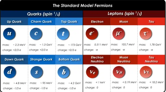
Figures 2.1 and 2.2 depict the Standard Model fermions and bosons, respectively. All par- ticles are shown in groups, and the three different generations of the fermions are highlighted by the use of different shades. The charge, mass and quantum mechanical spin are summarized in these figures

. To each of the fermions, save perhaps the neutrinos

, there corresponds an oppositely charged anti-particle with many similar properties including the quantum mechanical spin and mass. The anti-particles themselves are not shown explicitly in the figure, but their inclusion is implied.

1

The convention adopted in the present analysis is to work in units such that c = ~ = 1. All values listed in the figures are measured values from the Particle Data Group (PDG) summary tables [3], with the exception of the Higgs Boson mass in Figure 2.2, which comes from a combined ATLAS and CMS measurement [4].

2

Should neutrinos turn out to be majorana particles they will be their own anti-particles.

3

2.1 The Standard Model of Particle Physics 4

The Standard Model Fermions

Up Quark

mass: ~ 2.3 MeV charge: +2/3 e

u

Charm Quark Top Quark Electron Muon Tau

Quarks (spin ¹/2) Leptons (spin ¹/2)

Down Quark Strange Quark Bottom Quark Electron

Neutrino Muon

Neutrino Tau

Neutrino

c t

mass: ~ 1.3 GeV charge: +2/3 e

mass: ~ 173 GeV charge: +2/3 e

mass: ~ 4.8 MeV charge: -1/3 e

d s b

mass: ~ 95 MeV charge: -1/3 e

mass: ~ 4.2 GeV charge: -1/3 e

mass: 0.511 MeV charge: -e

e ^- 𝝁 ^- 𝛕 ^-

mass: 105.7 MeV charge: -e

mass: 1.78 GeV charge: -e

mass: < 1 keV charge: 0

𝝂 ^e 𝝂 ^𝝁 𝝂 ^𝛕

mass: < 0.19 MeV charge: 0

mass: < 18.2 MeV charge: 0

Figure 2.1: The quarks and leptons making up the fermions of the Standard Model.

Gluons (spin 1)

(Strong Interaction)

Higgs Boson (spin 0)

(Mass Coupling)

W⁺/W^- and Z Bosons (spin 1)

(Weak Interaction)

The Standard Model Bosons Photon (spin 1)

(Electromagnetism)

mass: 0 charge: 0

𝜸 ^{W +}

mass: 80.4 GeV charge: +1 e

W ^-

mass: 80.4 GeV charge: -1 e

Z ⁰

mass: 91.2 GeV charge: 0

mass: ~125 GeV charge: 0

H

charge: 0

g g

g g

g g

g g

Figure 2.2: A summary of the various Standard Model gauge bosons, including the force mediators for the

electromagnetic, strong and weak nuclear forces. The Higgs boson, which is involved in the generation of the

masses of the matter particles via EWSB, is also included.

2.2 The Top Quark 5

2.2 The Top Quark

2.2.1 Role in the Standard Model

Speculation on the existence of the third-generation, positively charged weak-isospin doublet partner of the bottom quark – the top – came in 1997, shortly after the discovery of the bottom quark itself [5]; the bottom quark was discovered as a result of the observation of a series of heavy baryons and mesons suggesting the existence of quarks with masses beyond those of the up, down, charm and strange quarks [6]. The observation, nearly twenty years later, of pairs of top quarks

produced via the strong interaction in p-¯ p collisions was made jointly by the D0 and CDF collaborations [7] [8]; this was subsequently followed in 2006 by evidence, again by the D0 collaboration, of single top quark production mediated by charged weak-current interactions, with the subsequent observation confirmed by both Tevatron experiments in 2009 [9–11]. The centre-of-mass energy of the Tevatron at the time of the single top discovery was √

s = 1.96 TeV. The protons accelerated by the LHC and involved in the collisions at the centre of the ATLAS detector considered for the present analysis each have an energy of E

= 4 TeV, leading to a total centre-of-mass energy of √

s = 8 TeV.

In the recent years since the LHC has been the world’s highest-energy centre for collider physics, vast numbers of top quarks have been produced allowing for the measurement of the properties of what is now the heaviest of all known fundamental particles. As many as five million top quarks were produced, either singly or in t ¯ t pairs, in the centre of the ATLAS detector during the 2012 data-collection period; the LHC can consequently be referred to as a veritable top factory. While only a minor fraction of those top quarks produced ultimately end up being reconstructed as signal top quark candidates in the various analyses due to the efficiency of triggering and event selection requirements, substantial numbers of them remain to fill the final distributions of interest. Indeed, the recent years have witnessed a paradigm shift in many top quark-related measurements as systematic uncertainties now become dominant over statistical uncertainties.

2.2.2 Production Mechanisms

In high-energy collider physics, two useful quantities that determine the event rates for a given process are the luminosity and the cross-section. The luminosity is intrinsically an accelerator- dependent quantity and is a measure of the rate at which high-energy collisions occur. Units for the instantaneous luminosity, denoted as L, are cm

· s

. One can also speak of the integrated luminosity, L, which is simply the intantaneous luminosity integrated over a selected period of time. In general then, the instantaneous and integrated luminosities are related via :

3

Pairs in this case implies a top-antitop quark pair, often abbreviated as t t. ¯

2.2 The Top Quark 6

L = Z

Ldt (2.1)

The cross-section is rather a process-dependent quantity, denoted by σ, and represents, in a sense, a measure of the statistical probability of a particular process occurring. It has dimensions of area and is typically quoted in units of µb, nb or pb (micro- or nano-, or picobarns) where one barn is equal to 10

cm

. In the case of the proton-proton collisions at the centre of the ATLAS detector, the production cross-sections depend on the partonic centre-of-mass energy

√ ˆ

s available as a result of the inelastic scattering of parton

constituents from two oppositely directed protons

. The calculation of production cross-sections for a particular process of interest is necessarily an approximation to a given level of desired precision

and involves the addition of a large number of possible interactions via the perturbative machinery of Quantum Field Theory (QFT) [12]. It should be emphasized that in order to produce heavier particles, such as top quarks, it is necessary that the energy available, √

ˆ

s, be above a production threshold, dictated by the rest mass(es) of the particle(s) to be produced.

For the generic process pp → X, the number of expected events to be produced as a result of collisions over the relevant time interval is dictated by the relation:

N

= Lσ

(2.2)

Figure 2.3 shows the peak instantaneous luminosities measured at ATLAS over the three years of the Run I data-collection period. The largest value can be seen to be approximately 8 × 10

cm

· s

or, equivalently, 0.008 pb

· s

.

Provided there is sufficient energy in the hard-scatter event resulting from a p-p collision, i.e. provided √

ˆ

s & 2m

where m

is the top quark mass, it becomes kinematically possible

to produce a top and anti-top quark pair. The dominant production mechanism at the LHC involves a gluon-fusion process – the interaction of two gluons, each originating from one of the colliding protons – and mediated by the exchange of either a third gluon via a triple gluon coupling in an s-channel interaction, or a virtual quark in a u- or t-channel interaction

. Alternatively, a valence quark from one proton annihilates with an anti-quark from the other proton, thereby producing a t t ¯ pair mediated by the exchange of a virtual gluon, either via an

4

The term parton refers to the constituents of the proton and is therefore used as a general term to denote either a quark or a gluon.

5

For the scattering of two partons, labelled 1 and 2, each with momentum fraction x

and x

of their respective protons, the centre-of-mass energy available will not be √

s = 8 TeV, but rather √ ˆ

s where ˆ s = x

x

s.

6

Theoretical calculations are commonly performed at Next-to-Leading or Next-to-Next-to-Leading Or- der (NLO or NNLO).

7

The Mandelstamm variables s, t and u arise in 2 → 2 scattering processes (though not limited to such

cases) and correspond to different permutations of four-momentum transfers between the incoming and outgoing

bodies involved. In the present context they are used to differentiate between graphical representations of the

interactions in the form of Feynman diagrams. For more information see, for example, [12], [14] or [3].

2.2 The Top Quark 7

Figure 2.3: The measured peak instantaneous luminosities at ATLAS during Run I [13].

s- or t-channel, in a process referred to as quark-antiquark annihilation.

Both the gluon-fusion and quark-antiquark annihilation processes are possible at the LHC, though their relative contributions depend on the energy available in the scattering process [3].

During 2012 ATLAS data-taking at a centre-of-mass energy of √

s = 8 TeV, the contribution from gluon-fusion production of t t ¯ pairs was roughly eight times larger than that from the q q ¯ annihilation process for reasons that will become clear in what follows.

2.2.3 The Partonic Structure of the Proton

An understanding of the composite nature of a proton is of paramount importance in the study of processes from hadronic collider interactions. The partonic (quark and gluon) structure of the proton has been studied extensively, and is described in the framework of the so-called Parton Distribution Functions (PDFs) [3]. These functions, measured by data via lepton- nucleon scattering experiments, mathematically describe the expected fractional contribution from each flavour of parton in the makeup of the proton, evaluated in a particular energy regime. This fact is important, as it is the interactions between the individual partons, and not the protons as a whole, which are relevant to the production mechanisms for t t ¯ pairs in a given collison event [15,16]. Figure 2.4(a) shows an example of the measured CT10 parton distribution functions of the proton which were used during the production of the simulated signal samples used in this analysis

.

The total probability of selecting a parton of any flavour in the proton is subject to the normalization constraint:

8

The all-hadronic t ¯ t signal process will be described in detail in Chapter 5.

2.2 The Top Quark 8

x

10

10

10

10

1

)

µ x f(x;

10

10

1

10

13 TeV 8 TeV

u d u d

g s c b CTEQ 6.6

= 161 GeV µ

) = 0.118 (mZ

αs

CT10

(a) Examples of the CT10 proton parton distribution functions (PDFs) employed in this analysis, describing the probability a particular parton type with fraction x of the incoming proton momentum being involved in a given hard-scattering process. The particular PDFs shown as a function of x are evaluated at a factoriza- tion scale µ = 161 GeV. The various coloured lines correspond to different parton flavours. The widths of the lines correspond to uncertainties in the values of xf

(x; µ

) for parton flavour i. The meaning of the three dotted vertical lines is explained in the text.

xi

0.1 0.2 0.3 0.4 0.5 0.6 0.7 0.8 0.9 1

Productiont for t jMinimum x

0 0.05 0.1 0.15 0.2 0.25

= 1.96 TeV s Tevatron @

= 8 TeV s LHC @

= 13 TeV s LHC @

(b) Top quark pair production thresholds, repre- sented by the minimum required momentum fraction of one parton as a function of the momentum fraction of the other, presented for three different hadron col- lider configurations. Note that lines represent thresh- olds only – production of t ¯ t pairs would also be pos- sible at any values of (x

,x

) above the corresponding lines. The reference value of the top quark mass is taken to be m

= 172.5 GeV.

Figure 2.4: Sample distributions illustrating the concept of the proton PDFs as well a representation of the t ¯ t production theshold for three hadron collider scenarios.

X

i

Z

xf

(x; µ

)dx = 1 (2.3)

where the sum is performed over all parton flavours. The partonic structure of anti-protons

such as those involved in the p-¯ p Tevatron collider differ from those of protons, but similar such

PDFs exist in either case. Concerning the quark-related makeup of the protons involved in the

LHC collisions, in order to yield a final state |uudi and satisfy baryon conservation, a necessary

requirement is that:

2.2 The Top Quark 9

Z

f

(x; µ

) − f ¯

(x; µ

) dx =



 

 

2 when i = u 1 when i = d 0 when i = s, c, b, t

(2.4) In the above equation the index i denotes the particular quark flavour, and the forms of f

(x; Q

) and ¯ f

(x; µ

) are meant to highlight parton distribution functions for a given quark flavour and its associated anti-quark flavour, respectively.

Figure 2.4(b) illustrates the role of the centre-of-mass energy of a hadron collider, notably in the context of the threshold requirement for the production of a t t ¯ pair, namely: √

ˆ

s = 2m

. This requirement can be expressed in terms of the two proton momentum fractions, x

and x

for partons i and j , as a requirement that x

and x

satisfy:

x

x

= 4m

s or x

=

2m

√ s

1

x

(2.5)

This value of x

is plotted as a function of x

for different values of √

s corresponding to three different hadron collider configurations. One can clearly observe that the product x

x

can be substantially lower in the case of the LHC compared with the Tevatron, particularly during Run II conditions at a higher centre-of-mass energy, while still satisfying the threshold requirement for t ¯ t production. With such low momentum fractions and in light of the parton distribution functions of the colliding protons shown in Figure 2.4(a), the probability of an interaction involving a gluon pulled from the parton sea far exceeds that of a quark or anti-quark.

Quark-Antiquark (qq) Annihilation_

Top Quark Production @ ATLAS

Leading-Order (LO) Single Top Production Modes LO tt Production Modes

At LHC gg fusion dominant

~87% @ √s = 8 TeV

-

q t

W

b -

q - t

q W b

q’

t t

W

W

b b

t g b

g q

-

q g

g

g g g

g

t t

t- t-

t- t

t

s-Channel t-Channel Wt-Channel Gluon Fusion

Figure 2.5: The dominant production modes of top quarks at the LHC.

By the same reasoning, the gluon-fusion process can be expected to play an even more

significant role as the available energy in the collision increases. The dotted vertical lines in the

2.2 The Top Quark 10

plot of Figure 2.4(a) show the values of x required to produce a t ¯ t pair in the case that both momentum fractions are equal, i.e. in the case where x

= x

. From Equation 2.5 these have values given by x = 2m

/ √

s. The values shown correspond to the two Run-I centre-of-mass energies of the LHC ( √

s = 7 and 8 TeV) and that for the initial Run-II data-taking period ( √

s = 13 TeV). In this case a top quark mass of m

=172.5 GeV is assumed. An inspection of the lines confirms that at a higher centre-of-mass energy the t ¯ t production threshold becomes significantly lower relative to the total √

s = 13 TeV available in the collisions; one can conclude that during Run II data-taking only a very small relative fraction of the t t ¯ pairs will be expected to be produced via q q ¯ annihilation – gluon-fusion is far more likely to occur in a given interaction as the gluons in the colliding protons are more accessible for interactions.

In the case of the Tevatron experiments, where p-¯ p collisions allow for the quark-antiquark annihilation mechanism from valence quarks alone, it is rather the q q ¯ annihilation process which dominates the production of t ¯ t pairs.

It should be highlighted that at LHC energies, the t ¯ t production threshold is so low relative to the total energy available in a typical interaction that the t ¯ t pairs are often produced with a significant boost

; this has implications in the strategies used in the offline reconstruction of top quark candidates.

Figure 2.5 illustrates some leading-order production modes of top quarks at the LHC exper- iments such as ATLAS. The dominant production mechanisms for both single top quarks and top quark pairs are shown [17].

A recent measurement of the total inclusive t t ¯ production cross-section was made in the dileptonic (eµ) channel by ATLAS

, specifically searching for events with oppositely charged high-p

electrons and muons

[18]. The analysis resulted in a measured value of σ

= 242.4±1.7 (stat) ± 5.5 (syst) ± 7.5 (lumi) ± 4.2 (E

) pb, using the √

s = 8 TeV dataset

. This value is consistent with recent theoretical NNLO and NNLL Standard Model predictions [19–22]. From this value of σ

, together with the instantaneous luminosity shown in the plot in Figure 2.3, one can estimate that at peak instantaneous luminosity during the 2012 data-collection period, as many as two pairs of top quarks were produced per second.

The total production cross-section for t ¯ t pairs in ATLAS can be expressed in the form [23]:

σ

√ s, m

= X

i,j=q,¯q,g

Z

dx

dx

f

(x

, µ

)f

(x

, µ

)× σ ˆ

ρ, m

, x

, x

, α

(µ

), µ

(2.6)

9

The boost of a particle is a measure of its energy relative to its rest mass. For a particle with mass m and energy E the boost is characterized by the familiar Lorentz factor γ = E/m.

10

The decay channels of t ¯ t pairs will be outlined in detail later in the chapter.

11

The transverse momentum p

will be defined in the following chapter.

12

The uncertainties (lumi) and (E

) in the measured value of the cross-section correspond to uncertainties

in the total collected integrated luminosity and the LHC beam energy, respectively.

2.2 The Top Quark 11

where the sum is taken over all possible subprocesses, each evaluated at an energy scale µ; the indices ij can therefore represent gg (gluon fusion) or q q ¯ (quark-antiquark annihilation), but also the less dominant qg or ¯ qg production modes of t ¯ t pairs. The cross-section for a given subprocess, ˆ σ

, is expressed as a function of several variables including ρ =

ˆ

s

and the strong coupling constant α

. A higher top quark mass results in a larger production threshold;

the cross-section can consequently be expected to decrease. The presence of the top quark mass in this expression suggests that the inclusion of higher-ordered corrections to this expression and the reduction of overall additional uncertainties could allow for an indirect measurement of the top quark mass to be made from that of an inclusive cross-section σ

measurement alone

.

Figure 2.6: A selection of the production cross-sections for a selection of processes of interest at ATLAS. Shown are both theoretical values and those measured at LHC centre-of-mass energies of either √

s = 7 TeV (in blue) or √

s = 8 TeV (in orange). The widths of the bands denote the total uncertainty on the particular values. The numerical values listed beside each point correspond to the total integrated luminosity of the dataset used in performing the measurement [25].

For the sake of comparison the inclusive production cross-sections for a selection of processes of interest at ATLAS are shown in the plot in Figure 2.6, showcasing the relative production rates of t ¯ t pairs compared with other Standard Model processes. Shown are both the theoretical values, overlaid with recent measurements made using ATLAS Run I data at both √

s = 7 TeV

13

Such a measurement was made with early ATLAS data based on the results of a cross-section measurement,

obtaining a total precision on m

of approximately 5% [24].

2.2 The Top Quark 12

and √

s = 8 TeV.

From the plot one can observe the inclusive W and Z boson production cross-section to be two to three orders of magnitude above that of t t ¯ pairs – evidence of the large role played by these processes as backgrounds in several analyses, particularly those involving single top quarks produced via the electroweak interaction where signal and background signatures are difficult to distinguish from one another. The dominant production mode of single top quarks at the LHC is via a t-channel production mode, which one can also note from the plot to be a few times smaller than the total t ¯ t production cross-section; top quarks are produced more often in pairs at the LHC than singly. The fact that t ¯ t production is quite large compared to many other Standard Model processes of interest at the LHC results in t ¯ t production serving as a significant background process to the signal processes in a number of physics analyses. This is also true for many Beyond the Standard Model (BSM) type theories, where t ¯ t processes represent the largest proportion of background event.

The results of various LHC measurements of the inclusive t ¯ t cross-section, as well as a com- bination from measurements made from the Tevatron experiments, are highlighted in the plot in Figure 2.7

. All measurements can be seen to be consistent with the Standard Model pre- dictions. The ATLAS-only results for single top quark production cross-section measurements, all in agreement with the Standard Model, can be seen in Figure 2.8.

14

The t ¯ t differential production cross-section has also been measured – the production cross-section as a function of several detector observables – using ATLAS √

s = 7 TeV data [26].

2.2 The Top Quark 13

[TeV]

s

2 3 4 5 6 7 8 9

cross section [pb]tInclusive t

1 10 102

103

ATLAS+CMS Preliminary TOPLHCWG

Sep 2014

* Preliminary

-1) Tevatron combined* 1.96 TeV (L=8.8 fb

-1) ATLAS dilepton 7 TeV (L=4.6 fb

-1) CMS dilepton 7 TeV (L=2.3 fb

-1) ATLAS l+jets* 7 TeV (L=0.7 fb

-1) CMS l+jets 7 TeV (L=2.3 fb

-1) ATLAS dilepton 8 TeV (L=20.3 fb

-1) CMS dilepton 8 TeV (L=5.3 fb

-1)

* 8 TeV (L=5.3-20.3 fb µ

LHC combined e

-1) ATLAS l+jets* 8 TeV (L=5.8 fb

-1) CMS l+jets* 8 TeV (L=2.8 fb

NNLO+NNLL (pp) ) p NNLO+NNLL (p

Czakon, Fiedler, Mitov, PRL 110 (2013) 252004

uncertainties according to PDF4LHC αS

⊕ = 172.5 GeV, PDF mtop

7 8

150 200 250

Figure 2.7: Summary of recent top quark pair production measurements, σ

, shown as a function of centre of mass energy √

s. Theoretical values are indicated by solid lines, with uncertainties represented by coloured bands. The inset figure, with the y-axis no longer on a logarithmic scale, shows an enlarged view of the two sets of measurements from the LHC experiments [27].

[TeV]

s

5 6 7 8 9 10 11 12 13 14

[pb] σ single top-quark cross-section

1 10 10

t-channel Wt

s-channel

MSTW2008 NNLO PDF = 172.5 GeV NLO+NNLL at mt

stat. uncertainty

arXiv:1406.7844

t-channel 4.59 fb-1

ATLAS-CONF-2014-007

t-channel 20.3 fb-1 PLB 716 (2012) 142

Wt 2.05 fb-1

ATLAS-CONF-2013-100

Wt 20.3 fb-1

arXiv:1410.0647

s-channel 95% C.L. limit 20.3 fb-1

ATLAS-CONF-2011-118

s-channel 95% C.L. limit 0.7 fb-1

ATLAS Preliminary October 2014

single top-quark production

Figure 2.8: Summary of recent ATLAS single top quark cross-section measurements, σ

, shown as a function of centre of mass energy √

s. Theoretical values are indicated by solid lines, with uncertainties represented by

coloured bands. Shown separately are the three production modes for single top quarks: t-channel, s-channel,

and the Wt associated production channel [27].

2.2 The Top Quark 14

2.2.4 Decay Modes

Once produced, top quarks will nearly always decay via t → W b, with the Standard Model branching ratio (BR) for such a process (as compared with other top quark decay channels) being greater than 99%; the CKM

-suppressed BR(t → W s) is at the per mil level and BR(t → W d) an order of magnitude below that

[23]. The decay of a t ¯ t pair will therefore nearly always result in an intermediate state W

bW

¯ b.

- -

2 Hadronic Decays

2 Leptonic Decays

Single Decay Diagrams

Categorization of W Boson Decays

Leptonic Decay Hadronic Decay

-

Two Decays

2 Leptonic 1 Leptonic 1 Hadronic 2 Hadronic

- _

Leptonic Decay Hadronic Decay

-

(BR ~ 32.4%) (BR ~ 67.6%)

Two Decay Diagrams

1 Leptonic/1 Hadronic

-

(BR ~ 10.3%) (BR ~ 43.5%) (BR ~ 46.2%)

Figure 2.9: A depiction of the leptonic and hadronic decays of a real Standard Model W boson, as well as pie charts illustrating the fractional decay categorizations in the case of a single or pair of W bosons. Values quoted are from [23].

The W bosons, in contrast, are less partial to a single particular decay mechanism as in the case of the top quark decays; a W boson will either decay leptonically (with a decay of the type W → `ν) or hadronically (via W → q q). Measurements have found the respective ¯ branching ratios for each of these processes to be 32.4% and 67.6%, in agreement with Standard Model theoretical predictions. Since there are two W bosons in each t ¯ t decay, three unique decay scenarios present themselves: both W bosons decay leptonically, both decay hadronically, or a decay of each type occurs. The decay channels of the t t ¯ pairs are thus characterized by the subsequent decays of the two W bosons and are designated, respectively, as the dileptonic

15

The values of the Cabibbo–Kobayashi–Maskawa matrix effectively represent the mixing of quark between the various generations and flavours. For more information refer to the Particle Data Group summary [3].

16

The strength of the vector-minus-axial-vector (V-A) charged-current W tb vertex in the Standard Model is given by

−i

V

γ

(1 − γ

)

, where V

is the corresponding term in the CKM quark-mixing matrix.

2.2 The Top Quark 15

channel, the all-hadronic or fully hadronic channel, and the semileptonic or lepton+jets (` + jets) channel.

Figure 2.9 illustrates the decay mechanisms of the Standard Model W boson, with pie charts depicting the branching ratios of the leptonic and hadronic W -decays, as well as the categoriza- tions involving a pair of W bosons (or equivalently, top quarks). The values of the branching ratios of t ¯ t pairs are summarized explicitly in Table 2.1.

Table 2.1: A summary table of the dominant decay channel classifications for top-antitop quark pairs including the associated branching fraction for each channel. Values quoted are from [23].

Decay Channel Process Branching Ratio [%]

Dileptonic t t ¯ → W

bW

¯ b → `νb`ν ¯ b 10.3%

Semileptonic t ¯ t → W

bW

¯ b → q qb`ν ¯ ¯ b 43.5%

All-Hadronic t ¯ t → W

bW

¯ b → q qbq¯ ¯ q ¯ b 46.2%

Each of these three t ¯ t decay topologies presents their own set of both advantages and dis- advantages from an experimental point of view. It should be noted that although in principle the branching ratios for the dileptonic and semileptonic channels include all possible lepton flavours, in the case of W bosons decaying via W → τ ν

, the subsequent decays of the tau particles are often more difficult to identify, and in general the term lepton in ‘lepton+jets’ is taken to correspond only to electrons and muons (i.e. ` = e, µ only).

Dileptonic t ¯ t Channel

The dileptonic t t ¯ channel is characterized by extremely low backgrounds, which consist primarily of cases of fake or misidentified leptons [28]. The presence of two high-energy, non-interacting neutrinos makes it difficult to infer their respective four-vector quantities from the missing energy in the detector. Consequently a full event reconstruction of the t t ¯ system is not possible; an over-constrained set of equations is often used to infer the neutrino energies. The low branching ratio also results in limited statistics for this channel.

Semileptonic t ¯ t Channel

In the semileptonic or `+jets t ¯ t channel, an ambiguity arises in terms of which of the two bottom-quarks

are to be associated with which reconstructed W boson – an issue referred to

17

It is in fact a reconstructed object referred to as a jet which is associated with each bottom-type quark in

ATLAS. This will be the topic of Chapter 4.