A Continuous Solution to the Norming Problem

(1)

Assessment 1 –14

sagepub.com/journalsPermissions.nav DOI: 10.1177/1073191116656437 asm.sagepub.com

Article

A good quality psychometric test has to satisfy certain criteria, usually defined as objectivity, validity, and reliability (e.g., Anastasi & Urbina, 1997). However, another important facet exists that is seldom explored in detail, yet is often equally vital to the testing process—namely, the way a test is actually normed.

Clearly, when tests are mastery or criterion-referenced, they do not require norms, for example, those assigning com- petence levels to person parameters (e.g., proficiency scaling in the Programme for International Student Assessment).

However, for the vast majority of psychometric constructs, the comparison with a representative norm is crucial. This is especially true when group-based studies and large-scale assessments are not available, such as in the field of applied diagnostics, when educational or clinical diagnosis at an individual level is required. Notably, diagnostic manuals often refer to percentiles when determining clinical disorders. For instance, the Diagnostic and statistical manual of mental disorders–Fifth edition (American Psychiatric Association, 2013, p. 69), although acknowledging that norm-referenced cutoff scores are somewhat arbitrary, states that academic skills below the 7th percentile are most consistent with specific learning disabilities. In many cases, remedial funding is only available if performance actually is below this pre- defined threshold. Although good psychometric and clinical practice need not rigidly adhere to cutoff scores and instead use a dimensional approach, it is still important to precisely assess deviation from the average. Furthermore, in educational and academic contexts, placement decisions, college admissions, or the assessment of special educational needs

to rely on interindividual comparisons of the students’ per- formances relative to others. Hence, the development of optimal norming procedures is necessary.

Challenges of Test Norming

Two major tasks confront the researcher when norming a test, both of which we describe in some detail to lay the foundation for a continuous approach and for readers who might not be familiar with the specifics. First, a suitable standardization sample must be recruited and second, a suitable norm score from the raw data must be estimated.

Problems of Data Collection

Recruiting a standardization sample that is representative of the target population presents formidable challenges (cf.

Gregory, 1996). As in experimental designs, confounding variables and noise factors potentially influencing the test scores have to be identified. Such variables might include age, sex, ethnic group, or geographic region.

1Psychometrica, Institute for Psychological Diagnostics, Dettelbach, Bavaria, Germany

2University of Wuerzburg, Bavaria, Germany

3University of Regensburg, Bavaria, Germany

4University of Basel, Suisse, Switzerland Corresponding Author:

Wolfgang Lenhard, Department of Psychology IV, University of Wuerzburg, Bavaria 97074, Germany.

Email: wolfgang.lenhard@uni-wuerzburg.de

A Continuous Solution to the Norming Problem

Alexandra Lenhard

¹

, Wolfgang Lenhard

²

, Sebastian Suggate

³

, and Robin Segerer

⁴

Abstract

Conventional methods for producing test norms are often plagued with “jumps” or “gaps” (i.e., discontinuities) in norm tables and low confidence for assessing extreme scores. We propose a new approach for producing continuous test norms to address these problems that also has the added advantage of not requiring assumptions about the distribution of the raw data: Norm values are established from raw data by modeling the latter ones as a function of both percentile scores and an explanatory variable (e.g., age). The proposed method appears to minimize bias arising from sampling and measurement error, while handling marked deviations from normality—such as are commonplace in clinical samples. In addition to step-by-step instructions in how to apply this method, we demonstrate its advantages over conventional discrete norming procedures using norming data from two different psychometric tests, employing either age norms (N = 3,555) or grade norms (N = 1,400).

Keywords

continuous norming, data smoothing, curve fitting, norm scores, norm generation

(2)

If the effect of these variables on test scores is large and relevant to the interpretation of test results, the variables are often accounted for in norm tables as explanatory variables.

Thus, in talent assessment, age or grade are explanatory variables because the performance on intelligence or academic tests varies with the age or grade of an examinee. Therefore, such tests normally report either age or grade norms, which, however, poses a new challenge. Specifically, when age or grade relates strongly to test performance and the given test norms cover a large range of ages or grades, a corre- spondingly large number of subsamples has to be included in the standardization sample. For example, the Wechsler Intelligence Scale for Children®–Fifth edition (Wechsler, 2014) offers normative age brackets which span 4 months each. As the test ranges from age 6 years and 0 months to age 16 years and 11 months, norms for 33 age brackets are reported. Accordingly, to obtain a representative subsample for each age bracket would require a huge number of children, thus precluding and inhibiting test development.

Alternatively, it would be possible to enlarge the age or grade span of each age bracket, thus replacing 4-month brackets with 12-month brackets. Although more cost- effective, it would lead to errors for those examinees whose age markedly differs from the average age of their own normative age bracket (e.g., a child aged 10 years and 0 month is 6 months younger than the average 10-year-old).

Briefly, effective curve fitting techniques are needed to mathematically model the influence of important explanatory variables on the measured ability, which considerably reduces the total sample size required (cf. Zhu & Chen, 2011) and allows norm generation with high precision (e.g., age norms could be calculated down to the very day).

Problems of Norm Score Generation

The second task in establishing norms is to derive norm values from the raw score distribution of a test. While the first task (i.e., recruiting a representative standardization sample) is usually described in detail in test manuals and textbooks, the second one is only rarely dealt with in depth—if at all. For example, in the manual of the Kaufman Assessment Battery for Children™–Second edition (KABC-II; Kaufman & Kaufman, 2004), approximately 10 pages are dedicated to the very precise description of how the data were collected and how the standardization sample was stratified. This can be regarded as best practice. However, only one brief paragraph deals with the question of how the norm scores were derived from the raw scores (Kaufman & Kaufman, 2004):

. . . Smoothed subtest norms were then created on the basis of these raw scores. The first step was to calculate the scaled score (mean of 10, standard deviation of 3) corresponding to the actual midinterval percentile rank for each raw score value at each half-year or year of age. This had the effect of normalizing the score distribution at each age. Next, these scaled scores

were smoothed both vertically (within age) and horizontally (across ages) using a computer program created for that purpose. Smoothing proceeded iteratively until the criteria for smoothness were met. (p. 85)

The paragraph describes that after normalizing the data, mathematical techniques were not only used to model the relationship between intelligence and age (“horizontal smoothing”) but also to model the relationship between raw scores and derived norm scores (“vertical smoothing”).

However, the employed algorithms along with the criteria for “smoothness” were not sufficiently specified. This scant level of detail is not the exception but the rule in test manuals. Indeed, information about modeling the relationship between raw scores and derived norm scores is also absent from textbooks on test construction (e.g., Crocker & Algina, 1986; Gregory, 1996).

In fact, several difficulties present themselves when transforming raw scores into percentiles or normalized standard scores. One problem associated with the transformation of raw scores into percentiles is that the standardization sample almost never delivers percentile ranks for each raw score achievable in the test. The more extreme a test result and the smaller the standardization sample, the higher the probability of a “gap” in the transformation between raw scores and percentiles is. In the Wechsler Intelligence Scale for Children–Fifth edition, each normative age bracket includes 200 participants. Despite this generous sample size, there is a relatively high probability (p = .58) that all 200 participants achieve scores within 3 standard deviations of the mean (IQ score between 55 and 145). Expressed differently, there is only a 42% chance that, despite having a large norm sample, a single participant will have provided raw data for the extreme ends of the test (i.e., IQ < 55 or IQ > 145). To close the gaps, “vertical” modelling is needed, that is, modelling of the relation between raw scores and percentiles for any age bracket or level of explanatory variable.

A second problem in deriving norm scores also arises when extreme scores come into play: Extreme test results coupled with small standardization samples result in distortion in the assignment of percentiles to raw scores based on the distribution of the standardization sample. Three major sources of error account for this distortion: (a) sampling error, (b) a lack of sample representativeness, and (c) measurement error. Crucially, sampling error can occur even if the sample is perfectly stratified and the measurement error is low. In such cases, sampling error arises from random variation in the selection of individuals from a given population and constitutes an additional error source solely related to test norms and not to measurement errors. When drawing random samples of N = 100 from a perfectly normally distributed population (M = 100 and SD = 15), in 95%

of all cases, the percentile rank of five lies between 76 and 87, thus spanning more than two thirds of a standard deviation.¹ In contrast, the equivalent interval around the 50th percentile ranges approximately from 97.5 to 102.5,

(3)

spanning only one third of a standard deviation. Crucially and as already pointed out, these intervals are not based on measurement error (i.e., on the reliability of a test), but are simply a consequence of sampling error in relation to extreme scores. In the context of psychometric testing and norming, this simple mathematical phenomenon puts additional uncertainty into a test result—uncertainty that is rarely quantified in psychometric tests.

The second source of error, namely the lack of sample representativeness, essentially belongs to the problem of data collection. Although this point was already described earlier qualitatively, we want to give a quantitative example here. Let us assume a hypothetical test yielding normally distributed raw scores in the reference population (M = 100 and SD = 15) but whose normative sample was not representative (M = 95, SD = 10). Whereas the error caused by a wrong average raw score of the standardization sample is constant for all locations, a nonrepresentative standard deviation of 10 instead of 15 points again has more impact for the extreme scores. For example, a child with a raw score of 105 and therefore having a true z-score of 0.33 lies at z = 1.0 on the unrepresentative subsample (i.e., 10 points above the norm mean of 95). A child with a raw score of 125 and, hence, receiving a true z-score of 1.67 would be at z = 3.0 on this nonrepresentative test norm—demonstrating an inflation of norming error for more extreme locations.

Finally, the third reason for erroneous transformations between raw scores and person locations arises from measurement error caused by inadequate test reliability. On an individual basis, measurement error is normally highest for extreme test performance and smallest around the midpoint of the raw score distribution—an effect that is so far adequately addressed mainly within item response theory approaches (cf. Klauer, 1991). Additionally, as far as the norm sample is concerned, extreme standard scores are based on scarce observations. Therefore, the empirical standard scores vary most extremely around the true population value for extreme person locations.

As described next, mathematical models have the potential to better estimate the relationship between raw scores and person locations than conventional norming techniques while reducing the norming error, removing discontinuous jumps, smoothing out distortions in subsamples, and using context information from adjacent age brackets or subsamples to adjust the shape of the distribution—which may have particular benefits for extreme test scores.

Continuous Norming: A Solution to the Mentioned Problems?

First attempts at modeling the relation between raw scores, person locations, and additional explanatory variables to minimize norming errors were made by Gorsuch (1983, as cited in Zachary & Gorsuch, 1985). He suggested a parametric “continuous norming” procedure, which is illustrated in

Figure 1. As a first step, means and standard deviations of the raw scores are calculated for all age brackets or grades included in the standardization sample. Subsequently, polynomial regression is used to estimate means and standard deviations as functions of age or grade. Finally, norm scores (e.g., percentiles) are computed for any age or grade included in the standardization sample based on Gaussian probability density functions with the estimated means and standard deviations as parameters. Unfortunately, the last step is only valid (cf. Taylor, 1998) if the raw scores are in fact normally distributed. However, in psychometric scales, especially in those that cover wide age ranges, skewness of the raw scores seems to be widespread. Often, it is not possible to cover the whole proficiency range with items of adequate difficulty, resulting in floor or ceiling effects. Figure 1, which is based on the original test data presented in Example 1 of this article, gives an illustrative example. The leftmost distribution (Age Group 1) represents a relatively low age with no marked floor or ceiling effect. The raw scores at this age do not deviate significantly from normal distribution. Therefore, modeling the probability density of the raw scores with estimated mean and standard deviation from Step 2 and deriving percentiles out of the estimated distribution works well.

However, in Age Group 3, which represents a high age bracket for this standardization sample, the raw score distribution shows marked skewness in the form of a ceiling effect. This implies that in this age group, the empirical percentiles deviate significantly from the percentiles as indicated by the estimated Gaussian probability density function in Step 3. For example, the empirical percentile of 90 is allo- cated at a much lower raw score than the estimated one.

Therefore, if continuous norming is based on the assumption of normality, new kinds of norming errors come into play, which are again most prevalent for extreme test scores.

Recognizing the need for data smoothing, Van Breukelen and Vlaeyen (2005) used a variation of a regression-based parametric norming approach. Consistent with Gorsuch (1983, as cited in Zachary & Gorsuch, 1985), they modeled means of the raw score distributions, including, alongside chronological age, further predictors in their regression analysis to increase prediction accuracy for an individual participant. However, in contrast to Gorsuch, it is a key assumption of their method that the variances of the distributions are constant across the total range of predictors.

This assumption of homoscedasticity is probably only rarely fulfilled in psychometric tests, particularly in devel- opmental tests when younger children remain on the floor or older children reach the ceiling (cf. Figure 1).

As a potential solution to deviations from normality, different researchers (e.g., Cole, 1988; Cole & Green, 1992;

Rigby & Stasinopoulos, 2004, 2005, 2006) used so-called Box–Cox power transformations to convert skew or kur- totic data into normal distributions. These transformations have mainly been used to fit physiological variables such as height, weight (e.g., Cole, 1988), triceps skinfold (Cole &

(4)

Green, 1992), body mass index (Rigby & Stasinopoulos, 2005), or blood flow (Rigby & Stasinopoulos, 2006).

However, the approach only works for variables with small or moderate skewness. Unfortunately, most psychometric tests contain floor or ceiling effects at least in some age brackets. As a consequence, Box–Cox power transformations cannot be applied to these data successfully.

On the one hand, continuous norming seems to have many advantages, for example, it avoids artificial age boundaries and increases the precision of norm score estimation. On the other hand, up to now, no adequate methods exist that are able to deal with data markedly deviating from a normal distribution—which is often the case in norm- oriented psychometric tests. Accordingly, Sijtsma (2012) stated that continuous norming would be of “great interest to test construction but little psychometric research has been done so far to study the method” (p. 10).

In this article, a new approach is presented based on Taylor polynomials. Taylor polynomials (for a mathematical description, see Dienes, 1957) are a mathematical means

to numerically model any function as long as this function is smooth in a mathematical sense.² Therefore, normality and homogeneity of variance are no requirements for the use of Taylor polynomials. Indeed, parametric continuous norming as described previously in this article also draws on Taylor polynomials, namely, when means and standard deviations are modelled as functions of different predictors via polynomial regression. In contrast to these parametric procedures, we do not model the different distribution parameters separately as functions of age groups or grades. Instead, we use Taylor polynomials to directly specify the functional relation between raw scores, person locations, and age or grade at the same time, thereby minimizing the total mean squared error. Geometrically speaking, this approach approximates a hyperplane with the best fit to the data, while simultaneously smoothing the data and filling the gaps between distinct norm groups and missing empirical data for specific test outcomes. Notably, we do not need any assumptions on the distribution of the raw scores.

The method is completely nonparametric and, therefore, inherently more robust against deviations from normality.

Figure 1. Illustration of parametric continuous norming as proposed by Gorsuch (1983, as cited in Zachary & Gorsuch, 1985).

(5)

We endeavor to show that Taylor polynomials (a) can be applied to any form of raw score distribution including scales with floor or ceiling effects; (b) fit the data sufficiently well, even for extreme raw scores; (c) provide good results even with small sample sizes; and (d) can be applied easily with standard statistical software (see step-by-step guide and electronic supplemental material available online at http://asm.sagepub.com/content/by/supplemental-data).

It is demonstrated that using this approach reduces many forms of norming error that occur with conventional norming procedures and, therefore, enhances the quality of psychometric instruments.

Nonparametric Continuous Norming:

Introduction of a New Procedure

In the presented continuous norming approach the raw score r is modeled as a continuous function of person location l (i.e., percentile or normalized standard score) and an explanatory variable a (e.g., age or grade):

r= f( , )l a (1)

According to the mathematical theory of Taylor polynomials, the polynomial

r l a c l a_st ^s

s t k

( , ) t ,

=

∑

=

0 (2)

is a suitable estimation of r, with the integer k denoting a smoothing parameter (for the exact mathematical deriva- tion see supplemental material S1). The constants c_st can conveniently be determined by multiple regression with the raw score as dependent variable and all products l^sa^t (see Formula 2) as independent variables.

The procedure can easily be performed with any current data analysis software. In the following section, we will provide a step-by-step guide on how to perform nonparametric continuous norming and how to retrieve norm data (have a look at the electronic support material , which dem- onstrates the procedure step by step via example data material and an SPSS syntax file):

1. Split the norm sample into subsamples, for example, into grade levels. In case of continuous explanatory variables (e.g., age), build a discrete grouping variable (e.g., age brackets).

2. Determine the percentiles of the participants in each subsample. If necessary, the percentiles can be transformed into normalized standard scores (e.g., z-scores) using a rank-based inverse normal transformation.

3. Compute powers of the continuous explanatory variable a as well as of the person location l (i.e., percentile or standard score) for each participant within each subsample (i.e., a, a², a³, . . . a^k, l¹, l², l³, . . . l^k).

Compute all products of these powers (i.e., a¹l¹, a²l¹, a³l¹, . . . a^kl¹, a¹l², a²l², a³l², . . . a^kl², . . . a¹l^k, a²l^k, a³l^k, . . . a^kl^k). As a starting point, powers up to k = 5 might be appropriate. We later analyze changes in model fit up to power eight.

4. Run a stepwise multiple regression with all powers and products of powers of a and l computed in Step 3 as the independent variables and the raw score as the dependent variable.

5. Define the Taylor polynomial function according to Formula 2 by choosing the significant variables from the stepwise regression and taking their unstandardized beta weights as the constants c_st in the polynomial.

So far in this article, we have described how the raw score r is modeled as a continuous function of person location l (e.g., percentile or z-score) and explanatory variable a (e.g., age). The resulting formula is sufficient to create norm tables for test manuals. For example, to compute the lowest raw score pertaining to a T-score of 32 simply insert the lower boundary of the performance interval (i.e., l = 31.5)³ into Formula 2 together with the mean age of the considered age bracket and round it up to the next integer. Subsequently, to compute the highest raw score pertaining to a T-score of 32 insert the upper boundary of the performance interval (i.e., l = 32.5) into the formula and round it down to the next integer. This can be done for age brackets as narrow and norm scales as precise as suitable. However, in some cases, it might be preferred or necessary (and also be more intui- tive) to directly compute the norm score out of the specific raw score and age of an examinee. The easiest way to get to this inverse transformation of Formula 2 is an iterative one.

To this purpose, an additional sixth step is necessary:

6. Insert different values for l in Formula 2 until the raw score in question is approximated with sufficient precision.⁴

Example 1 Data

The procedure described above is illustrated with standardization data from a standard vocabulary test (A. Lenhard, Lenhard, Suggate, & Segerer, 2015). The standardization sample included N = 3,555 children and adolescents whose age ranged from 2.59 to 17.99 years (M = 10.43, SD = 3.34).

The sample was representative of the population in terms of gender, education, and ethnic background.

Data Fit and Extrapolation

Implementation of the Procedure

Step 1. Discrete age brackets were built from the con- tinuously distributed age variable. For our first analysis,

(6)

we used a breakdown of the sample into 15 normative age brackets, each spanning 12 months. We investigate later in this article the invariance of the procedure against different age spans of the normative age brackets.

Step 2. The location l of each participant was estimated based on the empirical raw score distribution within each age bracket. To this purpose, the percentile of each participant was read out of the raw score distribution (ranking procedure according to Blom, 1958) and transformed into a z-score using a rank-based inverse normal transformation. The resulting z-scores are called empirical z-scores (z_emp) in the following. The transformation from percentiles to z-scores is not necessary for the out- lined continuous norming procedure itself, but for the subsequent analyses.

Step 3. All powers of l (i.e., z-scores) and a (i.e., age) and all linear combinations of the powers of l and a were calculated up to the 8th power. To determine which smoothing parameter k (see Formula 2) provided optimal results, 8 different multiple regressions were performed with k ranging from 1 to 8. This meant that the number of predictors⁵ in the regression analyses varied from 3 for k = 1 to 80 for k = 8. While the model fit potentially increases with k, the same is true for the number of observations necessary for a regression analysis.

Therefore, k is essentially limited by the sample size. (In the SPSS example syntax, the maximum value for k is 5.) Moreover, if k gets too high, there is a danger of model overfit, in the sense of modeling sampling or measurement error (cf. section “Example 2—Cross-Validation”

in this article).

Step 4. All variables computed in Steps 1 and 2 were used as independent variables in a multiple regression.

The raw score served as the dependent variable. The inclusion of predictors was carried out stepwise until the inclusion of another predictor did not lead to significant changes (p < .05) of F for the entire model.

Step 5. All significant independent variables were subse- quently used as addends in the Taylor polynomial, each multiplied with the according beta weight from the regression analysis as determined by Formula 2.

Step 6. For our further analyses, it was also necessary to determine l as a function of r and a for each participant.

To do this, the additional Step 6 was carried out. To this purpose, we inserted in Formula 2, the exact age of each participant and subsequently ran through different values for l iteratively until the raw score of each participant was matched with a sufficiently high precision.

Results and Discussion. As can be seen in Table 1, the coef- ficient of determination reached its maximum of R² = .99 for k = 3. In other words, the inclusion of higher powers of age and location did not further improve the data fit at first glance. Figure 2 illustrates the results of the nonparametric

continuous norming procedure for four different values of k (3, 4, 5, and 6). All curves are smooth and fit the data well. Relatively large deviations from the empirical z-scores (displayed by the marks) can only be seen for a z-score of −2. This is probably an effect of high measure- ment error for very low raw scores as discussed in the introduction. As the suggested nonparametric continuous norming procedure uses context information of all performance levels to adjust the shape of one specific curve, it can be assumed that the smoothness of the models reflects the true population curve better than the empirical data.

While the coefficients of determination suggest that all models with k ≥ 3 fit the data equally well, Figure 2 and Figure 3 reveal that they differ when it comes to extrapolation to age ranges or person locations not included in the standardization sample. The statistical problem with extrapolation is that it cannot be evaluated with empirical data because they are not available, otherwise extrapolation would not be required. However, plausibility and data from external sources may give some hints as to whether a model is suitable. For example, the vocabulary test has 228 items.

Therefore, a model that adequately maps the ceiling effect of the test should not exceed raw scores of 228. From Figure 2, it can be seen that if extrapolated to the age of 19 years, this holds only true for the models with k ≥ 5. On the other hand, if k is too high (e.g., k = 6), the models contain intersecting lines for different z-scores, which cannot occur in manifest norming data due to the invariance of the order of percent ranks. Obviously, the model with k = 5 seems to be the best model as far as extrapolation to higher age ranges is concerned. Figure 3 depicts extrapolation to person locations not included in the standardization sample at age 16.

Again, it can be seen that if k is too small (e.g., k = 3), the model gives implausible values (raw scores >228) for very high person locations. On the other hand, if k is too high (e.g., k = 7), the Taylor polynomial displays a maximum raw score at a finite person location and then decreases to lower raw scores, which means that higher person locations are related with lower raw scores beyond this maximum point. This is a numerical effect that contradicts the defini- tion of person location. Therefore, this part of the function could not be used for real psychometric tests. For k = 7, the maximum raw score of 220 is reached at z-score = 2.5, for k = 6, the maximum raw score is 221, which is reached at a z-score of 2.9. For k = 5, the Taylor polynomial also Table 1. Coefficients of Determination for Different

Smoothing Parameters k.

k R R² Adjusted R²

1 .95 .89 .89

2 .99 .98 .98

≥3 .99 .99 .99

(7)

displays a maximum (r = 224), however, it is located at a very high z-score (z-score = 3.6) and the raw score decreases very slowly beyond that point. Therefore, it is of little psychometric relevance. Again, the model with k = 5 (i.e., that includes up to the fifth power of l and a) seems to be the most suitable one. In the following, this model is called the k5-model. The model includes 11 predictors (a, l * a, l² * a, l² * a², l³ * a, l³ * a³, l⁴, a⁴, a⁵, l⁵ * a, l⁵ * a⁵).

In the present section, it was shown that the suggested nonparametric norming procedure not only has the potential to map the empirical data precisely but also to go beyond

the empirical database and to deliver models that allow at least moderate extrapolation as far as both age and location are concerned.

Invariance of Nonparametric Continuous Norming Against Different Methods of Estimation of l

Differences between the age of the examinee and the mean age of the corresponding age bracket are a main source of norming-related error in individual test results (compare electronic support material S2). The extent of this error can Figure 2. Results of the nonparametric continuous norming procedure for different smoothing parameters k.

Note. The marks depict age-dependent raw scores as determined by rank-based inverse normal transformation per age bracket, while the lines illustrate the resulting Taylor polynomial for five different zscores with smoothing parameter k ranging from 3 (upper left chart) to 6 (lower right chart).

(8)

be all the greater with an increasing impact of the explanatory variable on test scores (e.g., due to fast development at a specific age). In order to reduce this problem, age brackets can be reduced to shorter time intervals. However, on the manifest level, practical reasons like the size of the necessary norm sample set boundaries. Moreover, smaller age brackets also entail more uncertainty with regard to the estimation of population parameters. Therefore, if age brackets of different size yielded different test results, it would be difficult to decide, which method should be preferred.

From a theoretical perspective nonparametric continuous norming should reduce measurement errors that stem from small sample sizes, because each data point of the continuous norm contains information not only from a single age bracket but from the whole sample. Hence, it should be relatively invariant regarding the method used to estimate the location of the participants in the sample. To test this hypoth- esis, we used four different methods to estimate the location of the participants. For the first two methods, we divided the sample into 15 age brackets that each comprised an age span of 1 year (Method 1a) versus 30 age brackets that each comprised 6 months (Method 1b). Subsequently, we estimated the location of each participant with rank-based inverse normal transformation. Method 2a and 2b were also carried out with rank-based inverse normal transformation. However, this time we used an individual age bracket for each participant that was based on a sliding window. For example, for Method 2a, we compared each participant with all participants of the sample that were up to 6 months younger or up to 6 months older than the participant. This means that like in Method 1a, the age bracket comprised an age span of 1 year, but the average age of the age bracket exactly matched

the age of the participant. Hence, the method eliminated the age-related norming error described in the previous section.

Method 2b corresponded to Method 2a. However, this time we used an age span of 6 months. Subsequently, we performed nonparametric continuous norming for all four methods. As the k5-model had turned out to be the best in the first analyses (i.e., with Method 1a), we also chose k = 5, for the other three methods. This procedure yielded four additional methods, namely Method 3a: k5-model, estimation of l based on Method 1a; Method 3b: k5-model, estimation of l based on Method 1b; Method 4a: k5-model, estimation of l based on Method 2a; Method 4b: k5-model, estimation of l based on Method 2a (also see Table 2 to get an overview of the different methods).

Data Analysis. As Method 2a could only be applied for par- ticipants who were at least 6 months older than the youngest participant or 6 months younger than the oldest participant, we restricted the analyses of this section to participants that were between 4 and 16 years old (n = 3,309). As a first step, we calculated the differences between the z-scores of the two versions of each method for all participants, that is, we compared Method 1a with Method 1b (=Δz-score₁), Method 2a with Method 2b (=Δz-score₂), Method 3a with Method 3b (=Δz-score₃), and finally, Method 4a with Method 4b (=Δz-score₄). Note that the variance of each Δz-score—not the mean, which was supposed to approach zero due to the rank-based normalization—indicates how strongly the two versions of one method deviate from each other and, therefore, how prone each method is to changes in the span of the age bracket. We compared the variances of the four Δz-scores inferentially (procedure according to Kristof, 1981) using the Bonferroni correction to adjust for multiple comparisons. The significance level was set to α = 5%.

As little differences between the two variations of one method would not guarantee a good quality of the method per se, we additionally analyzed the pattern of intercorrelations between the different methods. To this purpose, we calculated all pairwise Pearson correlation coefficients between the different versions of all methods (i.e., 1a, 1b, 2a, 2b, . . . 4b). Subsequently, we determined the average correlation between two methods (i.e., 1, 2, 3, and 4) according to the method of Olkin and Pratt (1958), which is less biased than the more common Fisher’s z transformation (cf. Eid, Gollwitzer, & Schmitt, 2010). For example, the average correlation between Method 1 and Method 2 was calculated out of the four correlations r_{1a, 2a}, r_{1a, 2b}, r_{1b, 2a}, and r_{1b, 2b}. Finally, we compared the six resulting average correlation coefficients with each other inferentially (procedure according to Eid et al., 2010). Again, we used the Bonferroni correction and a significance level of α = 5%.

Results and Discussion. As expected, the means of the Δz- scores approached zero. None of them exceeded 0.01 Figure 3. Extrapolation to very high or very low z-scores for

three different smoothing parameters k at age 16.

Note. Instead of z-scores the y-axis displays the according probability densities in order that the presented curves can be more easily compared with a normal curve. The grey area corresponds to z-scores below −2.0 or above 2.0.

(9)

z-scores. As far as the variances were concerned, the varia- tion of the age span of each normative group had the greatest impact on Method 1. The variance of Δz-score₁ amounted to S² = 0.043, which means that the standard deviation spanned about one third of the size of the 95% confidence interval of a test result. The variance of Δz-score₂ was S² = 0.009, which was significantly lower than that of Δz-score₁, t(3307) = 50.13, p_adj < .001. This result suggests that the age-related norming error of Method 1 considerably contributed to the differences between Methods 1a and 1b. However, as pre- dicted, the impact of varying the age span of the normative age brackets was still substantially reduced when applying nonparametric continuous norming. Method 3 (S² = 1.94 * 10⁻⁴) as well as Method 4 (S² = 9.20 * 10⁻⁴) showed significantly lower standard deviations of the corresponding Δz- scores than Method 2, t(3307) = 192.38, p_adj < .001, for Method 3 and t(3307) = 81.29, p_adj < .001, for Method 4.

Note that the standard deviation of Δz-score₁ was approximately 15 times as high as that of Δz-score₃, indicating that Method 3 delivers results that are much more independent of the age span and sample size than those of Method 1.

Table 2 lists the intercorrelations between the z-scores gained with the different norming methods. First of all, it must be stated that all correlations are extremely high (>.97). This shows that none of the methods delivers results that strongly deviate from the results of the other methods.

Nevertheless, even high correlations between two methods can entail a large proportion of cases with significantly different test results on the individual level. In the electronic support material S2, we demonstrate a case where two different methods correlate as high as r = .9836, yet 4.4% of the cases show significantly deviating test results.

The test results gained with Methods 3 and 4 showed the highest average correlation with r = .9985. The correlation was significantly higher than that between Method 3 and Method 2, z = 53.87, p_adj < .001, and also significantly higher than that between Method 3 and Method 1, z = 65.66, p_adj < .001. Again, it can be clearly seen that the different versions of the nonparametric continuous norming procedure deliver very similar and stable test results. One could expect, at first glance, that the two empirical methods also deliver results that are very similar to each other and less similar to the results of the continuous norming models.

However, this is not the case. Instead, the test results gained with Method 2 correlate significantly lower with the results of Method 1 than with those of Method 3, z = −2.98, p_adj <

.05. The correlation between Method 2 and Method 4 is also higher than that between Method 2 and Method 1, however, the difference failed to reach significance, z = −1.04.

In summary, the data indicate that Method 1—probably the most common one used for generating test norms—is the method that is most prone to changes in the span of the age brackets and the sample size and in this respect delivers the most unreliable results. Moreover, it is the method that produces results which are most dissimilar to the ones of the other three methods. By contrast, the norms produced by nonparametric continuous norming are negligibly affected by changing the method to estimate l. The results are stable.

Moreover, they are very similar to another method, namely Method 2, which also prevents at least some forms of age- related norming error. However, there are several advantages of nonparametric continuous norming as compared with Method 2. First of all, Method 2 can only be applied with the help of special software (in our case, it was Table 2. Intercorrelations Between z-Scores Based on Different Methods Used to Estimate l.

Method 1 Method 2 Method 3 Method 4

1b 2a 2b 3a 3b 4a 4b

Empirical

Method 1: Common age brackets (“traditional approach”) .9889 .9848 .9844

Age span: 1 year 1a .9782 .9869 .9830 .9836 .9837 .9832 .9835

Age span: 6 months 1b .9930 .9927 .9860 .9860 .9852 .9856

Method 2: Individual age brackets (sliding window) .9899 .9893

Age span: 1 year 2a .9953 .9923 .9924 .9915 .9919

Age span: 6 months 2b .9875 .9875 .9865 .9871

k5-Model (Continuous norms)

Method 3: Common age brackets .9985

Age span: 1 year 3a .9999 .9980 .9990

Age span: 6 months 3b .9980 .9989

Method 4: Individual age brackets (sliding window)

Age span: 1 year 4a .9995

Age span: 6 months 4b

Note. The correlations printed in bold italics indicate average correlations determined according to the method of Olkin and Pratt (1958).

(10)

self-written software), whereas nonparametric continuous norming can be applied with standard statistical software such as R, SPSS, or STATISTICA. Second, nonparametric continuous norming uses information from the whole sample to derive each single norm score. This is not the case for Method 2. Therefore, although Method 2 is also able to pro- duce continuous norms, the results are more heavily affected by changes in the span of the age bracket and the sample size.

Example 2: Cross-Validation

So far in this article, we have analyzed how robustly empirical data can be modeled with our nonparametric continuous norming technique and how the model can help avoid age- related norming error. The next step is to test whether the model not only matches a specific sample drawn from a certain population but also fits a new sample from the same population. Moreover, we check whether norm values derived with nonparametric continuous norming fit a new sample better than do norm values derived from the old sample with a conventional norming technique. To this purpose, we reanalyzed data from a large standardization sample of a reading comprehension test based on grade norms (W. Lenhard & Schneider, 2006).

Data

The standardization data were collected during the years 2004 and 2005 and comprised a representative sample of 3,610 children from the beginning of Grade 2 to the beginning of Grade 5. For every grade, data were collected at two equidistant points of the school year, namely, at the beginning and in the middle. In this article, we only present the data of one subtest, namely, the sentence comprehension subtest. The maximum score in this subtest is 30 points. For every grade level (beginning of Grade 2, middle of Grade 2, beginning of Grade 3, . . . beginning of Grade 5), we randomly drew two nonoverlapping samples including n = 100 children out of the whole standardization sample, resulting in two different cross-validation groups with n = 700 children each. The two groups are called Cross-Validation Group 1 and Cross-Validation Group 2 in the following.

Data Analysis

The location l of each participant was estimated based on the empirical raw score distribution within each grade level of his or her own cross-validation group using the ranking procedure according to Blom (1958) and subsequent rank-based inverse normal transformation into T-scores (M = 50, SD = 10).

As in the previous analyses, these T-scores are called empirical T-scores in the following. The regression analysis was performed for each cross-validation group separately with

k = 5 and the raw score serving as the dependent variable.

Again, the inclusion of predictors was carried out until the inclusion of another predictor did not lead to significant changes (p < .05) of F for the entire model. We thus established a Taylor polynomial for each cross-validation group as described previously in the step-by-step guide.

As a next step, three additional T-scores were assigned to each participant. First, we calculated the T-scores for each participant based on the continuous norming models resulting from Cross-Validation Group 1 (T_mod1) and Cross- Validation Group 2 (T_mod2). Second, if possible, we also determined another empirical T-score for each participant, namely, the T-score which was related to his or her raw score, according to the raw score distribution in the cross- validation group he or she did not belong to. T-scores based on the raw score distribution of Cross-Validation Group 1 are called T_emp1, while T-scores based on the raw score distribution of Cross-Validation Group 2 are called T_emp2. Subsequently, we calculated the difference between both empirical T-scores (=ΔT_emp) and both modeled T-scores (=ΔT_mod). The variances of these differences were compared inferentially (procedure according to Kristof, 1981).

Furthermore, we computed correlations between the four different T-scores separately for each validation group and also compared them inferentially (procedure according to Eid et al., 2010). Again, we used a Bonferroni correction and a significance level (α = .05).

Results and Discussion

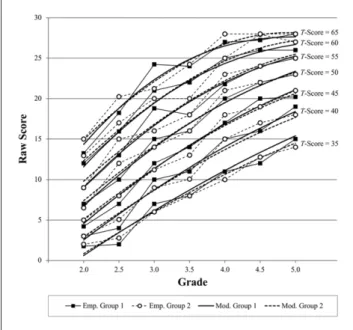
Figure 4 displays both the empirical results of the different cross-validation groups and the according continuous norming models. As can be seen from the figure, the model curves match each other fairly well and both display a smooth increase from Grade 2 to Grade 5. By contrast, the empirical data display serrated curves with negative slopes at some occasions (e.g., for Group 1, T-score 55 from Grade 3 to Grade 3.5). The quantitative analysis confirmed that the discrepancies between the two empirical T-scores (ΔT_emp: S² = 3.50) were larger than those between the modelled T-scores (ΔT_mod: S² = 0.81), t(1350) = 30.97, p < .001. This result again suggests that nonparametric continuous norming delivers more homogenous and stable results than conventional discrete norming.

The correlations between the different T-scores are displayed in Table 3. According to this analysis, T_mod1 and T_mod2 share about 99.2% of variance in each group, indicating that both models deliver almost identical T-scores.

In both groups, the correlation between T_mod1 and T_mod2 is significantly higher than that between T_emp1 and T_emp2, z = 15.32, p < .001, for cross-validation group 1 and z = 14.95, p < .001, for Cross-Validation Group 2. More important, in Cross-Validation Group 1, T_emp1 correlates significantly higher with T_mod2 than with T_emp2, z = 4.79, p < .001.

(11)

Accordingly, in Cross-Validation Group 2, T_emp2 correlates significantly higher with T_mod1 than with T_emp1, z = 2.68, p = .004. These results indicate that the models are better predictors of the raw score distribution of the other cross- validation group than are the raw score distributions of the own group.

Discussion and Summary

In this article, we presented a new, distribution-free approach for the calculation of continuous norms based on Taylor polynomials. The key findings—now briefly reca- pitulated—suggest that the current approach may provide a continuous solution to the norming problem.

Key Findings

First, it appears that the validity of conventionally established norms strongly depends on the age span of the normative age brackets, which, however, was not the case for norms generated with nonparametric continuous norming.

Moreover, there is the practical advantage that with nonparametric continuous norming robust norms can be produced with smaller sample sizes (also cf. Zhu & Chen, 2011). Consider for example, the test introduced in Example 1. We built 15 age brackets with approximately 240 cases each and retrieved norm tables for 51 distinct age brackets out of these. Conventional noncontinuous norming procedures would afford 51 × 240 cases (=12,570 cases) and still would not attain the same precision without applying further smoothing techniques. In some cases, the use of continuous norming might even facilitate the collection of standardization data. For example, many psychometric tests of school performance utilize grade norms that represent the typical performance at the end of the school year or at the end of a semester or trimester. To this purpose, standardization data have to be collected within a small time frame, which is often logistically difficult. With continuous norming, by contrast, standardization data can be collected the whole year round.

Second, we showed that our specific nonparametric continuous norming procedure delivers results that can predict the raw score distribution of a new sample more precisely than does the original raw score distribution. Furthermore, it avoids inadvertent effects like negative slopes for specific combinations of person location and age or grade in devel- opmental tests. Test developers using conventional norming procedures might smooth out such effects by hand.

However, there are neither precise rules as to when such effects are smoothed out nor how they are smoothed out in conventional norming. Moreover, given the difficulty of finding any test manuals describing the smoothing procedures underlying test norms, it appears that conventional norming lacks transparent and replicable procedures.

Third, we demonstrated that our approach not only shows high data fit but can also be used for moderate extrapolation to an age or person location not included in the standardization sample. Although extrapolation to person locations not included in the standardization sample is frequently applied in psychometric tests, the techniques Figure 4. Relation between raw score, location (T-score),

and grade in a reading comprehension subtest for two different cross-validation groups.

Note. Fine serrated lines with marks display the empirical results (filled marks for Group 1 and open marks for Group 2). Smooth lines display the models resulting from nonparametric continuous norming (dashed line for Model 2).

Table 3. Intercorrelations Between T-Scores Based on Two Different Cross-Validation Groups.

2 3 4

Cross-Validation Group 1 (n = 678) Empirical

1. Cross-Validation Group 1 .9795 .9868 .9849 2. Cross-Validation Group 2 .9820 .9843 k5-Model

3. Cross-Validation Group 1 .9961

4. Cross-Validation Group 2 Cross-Validation Group 2 (n = 674) Empirical

1. Cross-Validation Group 1 .9802 .9880 .9858 2. Cross-Validation Group 2 .9830 .9848 k5-Model

3. Cross-Validation Group 1 .9961

4. Cross-Validation Group 2

(12)

used to this end are poor at best. For example, in the widely used Children Behavior Checklist (Achenbach & Rescorla, 2001), the authors established a simple linear function between raw scores and T-scores for extreme test results, thereby using arbitrary minimum and maximum T-scores of 20 and 80 for the minimum and maximum raw scores.

Finally and most important, while the previous advantages also hold true for parametric continuous norming approaches, their drawback is to require assumptions on the distribution of the raw data, for example, normality and in some cases also homogeneity of variance across all levels of the explanatory variables. These drawbacks are over- come by our new nonparametric approach for which skewness or heterogeneity of variance play no role. In the presented example, we could even model a fairly pro- nounced ceiling effect at high age. Moreover, in analyses not presented in this article, the nonparametric continuous norming procedure was successfully applied to scales with even larger ceiling effects (e.g., the text comprehension subscale of the ELFE 1-6; W. Lenhard & Schneider, 2006).

Limitations and Practical Advice for Continuous Norming

It should be kept in mind that nonparametric continuous norming is a method that is not necessarily restricted to age or grade norms and performance tests. Performance data aside, it is also possible to use the method for the measurement of personality traits such as neuroticism or extraver- sion. Moreover, it is possible to include other covariates than age or grade. In principle, one could use any variable that covaries with the test scores (e.g., gender, ethnic origin, social background). Theoretically, it is even possible to include more than one explanatory variable, thereby gener- alizing the method to an n-dimensional approach. Critically, when using a Taylor polynomial with corresponding powers plus all interactions of powers of the independent variables, the number of predictors in the regression analysis quickly increases to an unmanageable quantity. Based on our experience with norming datasets additional to those reported in this article, the inclusion of a second explanatory variable works best when this additional variable is dichotomous instead of continuous (e.g., gender). However, in this case, model fit should be checked thoroughly—

especially at the extreme ends of the distributions.

Additionally, nonparametric continuous norming is also not restricted to the use of raw scores based on classical test theory. As any continuous function can be modelled with Taylor polynomials, our approach can equivalently be applied to latent trait scores.

Despite the advantages of nonparametric continuous norming, there are also some limitations and questions that need addressing the first of which concerns data fit. On the one hand, a model should of course map the empirical data

accurately. On the other hand, if the model is too close to the empirical data, it not only reproduces the true population parameters but also some of the errors inherent in standardization data with limited sample size or missing representativeness. Associated with this problem is the question of which method of multiple regression should be used. We applied multiple regression with stepwise selection of independent variables (=stepwise regression). The statistical procedure a posteriori determines those terms of the power series that uniquely contribute significant por- tions of variance. It is completely data driven and models the empirical data very closely. Some authors (Cohen, Cohen, West, & Aiken, 2003) have claimed that stepwise regression might lead to a data overfit. Unfortunately, a quantitative criterion indicating whether there is a data overfit does not exist. In our example, other methods (e.g., forward or backward selection of variables) did not yield appreciably different results. Therefore, stepwise regression seems to be one out of several different appropriate methods of multiple regression for performing nonparametric continuous norming. The cross-validation study further shows that the regression parameters and the T-values based on raw scores from two independent norming samples are fairly identical.

Another problem connected with multiple regression in general is the intercorrelation of the independent variables, which can severely hamper the interpretation of regression analyses. Moreover, Cohen et al. (2003) suggest to use data- set sizes with at least 40 times as many cases as the number of independent variables in the regression analysis in order to retrieve an invariant sequence of variables. For example, for two independent variables (e.g., person location and age) and k = 5 (=35 independent variables in the multiple regression) the total sample size would be at least 1,400.

However, these problems do not apply to our continuous norming approach, as we neither attempt to interpret the independent variables in terms of an explanatory theory nor require invariant sequences of the independent variables. In our experience, still lower numbers yet can suffice. For instances, the cross-validation of Example 2 yielded excel- lent results for as few as 100 cases per age group (i.e., only 20 times as many cases as the number of independent variables in the regression analysis). Furthermore, in many cases a lower smoothing parameter (k = 3 or k = 4) will be sufficient (e.g., W. Lenhard, Lenhard & Schneider, in press).

Another problem is extrapolation. As already described, extrapolation to person locations not included in the standardization sample is a somewhat widespread practice. For example, the standardization sample of the KABC-II (Kaufman & Kaufman, 2004) comprises N = 3,025 children. The standard scores (M = 100, SD = 15) indicated in the KABC-II range from 40 to 160. However, there is only a 31% chance that a single person out of 3,025 randomly chosen participants has a standard score of 155 or above.

(13)

The chance that none of the children has a standard score of 155 or above is more than twice as high (p = 69%). Although nonparametric continuous norming delivers values that are at least as plausible as the ones gained with other methods like, for example, Box–Cox transformations, the functional relation between raw scores and norm scores might not apply to extreme person locations. For this reason, we argue that extrapolation to extreme person locations should gener- ally be used very cautiously. In most cases, there is not even a reason to differentiate with such high precision. For example, in most cases, a child with a measured IQ of 145 would not be treated differently from a child with a measured IQ of 160. If extrapolation is nevertheless used in the construction of test norms, it should be more explicitly stated and described in the norm tables and manuals.

Interestingly, extrapolation to age ranges not included in the standardization sample is rarely seen in psychometric tests, although almost the same pros and cons hold true as for extrapolation to extreme person locations. As can be seen from Figure 2, nonparametric continuous norming does not always deliver plausible values for this kind of extrapolation.

We therefore recommend that the age range of standardization samples should be slightly wider than the age range reported in the statistical manual of the according tests. For example, in the vocabulary test of Example 1, the age range of the standardization sample was 2.59 to 17.99 years, while the test manual only reports norm scores for children from 3.0 years to 17.0 years. The norm scores of the upper and lower age brackets could then be determined more reliably.

Despite the aforementioned problems, nonparametric continuous norming seems to be a procedure, which can not only be easily applied with standard statistical software but also delivers stable and reliable norms. Therefore, we regard nonparametric continuous norming as a useful tool that can improve the quality of psychometric tests. It is a task of future work to further explore its limitations and benefits.

Author’s Note

The data presented in Example 2 constitute a subsample of the original standardization sample of ELFE 1-6 (W. Lenhard &

Schneider, 2006). The test manual contains test norms based on conventional norming.

Declaration of Conflicting Interests

The author(s) declared the following potential conflicts of interest with respect to the research, authorship, and/or publication of this article: The authors of the article receive royalties from sales of the test used in Example 1 (Peabody Picture Vocabulary Test 4, German version by A. Lenhard, Lenhard, Suggate, & Segerer, 2015). One of the authors (W. Lenhard) receives royalties from sales of ELFE 1-6.

Funding

The author(s) disclosed receipt of the following financial support for the research, authorship, and/or publication of this article:

Norming of the vocabulary test of Example 1 was funded by Pearson Assessment, Frankfurt, Germany, which also holds the copyright for the norms. Therefore, regression coefficients cannot be reported in this article. The method used to create the norms is also described briefly in the test manual. The reading comprehension test of Example 2 was funded by Hogrefe Verlag GmbH &

Co. KG, Göttingen, Germany.

Notes

1. This can be done via Monte Carlo simulations by repeat- edly generating N = 100 random number and determining the variation of the percentiles of the drawn samples or by approximating binomial distributions (e.g., Brown, Cai, &

DasGupta, 2001).

2. A function is smooth in a mathematical sense if it has deriva- tives of all orders. With regard to the graph, it means that the function has no angles or undefined points.

3. Beware that the used norm scale has to accord with the one used in the regression analysis.

4. Supplement 4 of the electronic support material includes a calculator that computes individual norm values and as well generates norm tables for specific age values.

5. The number of predictors amounts to k2 + 2k.

References

Achenbach, T. M., & Rescorla, L. A. (2001). Manual for the ASEBA school-age forms and profiles. Burlington: University of Vermont, Research Center for Children, Youth, and Families.

American Psychiatric Association. (2013). Diagnostic and statis- tical manual of mental disorders (5th ed.). Washington, DC:

Author. doi:10.1176/appi.books.9780890425596

Anastasi, A., & Urbina, S. (1997). Psychological testing (7th ed.).

Upper Saddle River, NJ: Prentice Hall.

Anonymous Authors (in press).

Blom, G. (1958). Statistical estimates and transformed beta- variables. New York, NY: Wiley.

Brown, L. D., Cai, T. T., & DasGupta, A. (2001). Interval estimation for a binomial proportion. Statistical Science, 16, 101-117.

Cohen, J., Cohen, P., West, S. G., & Aiken, L. S. (2003). Applied multiple regression/correlation analysis for the behavioral sciences (3rd ed.). Mahwah, NJ: Lawrence Erlbaum.

Cole, T. J. (1988). Fitting smoothed centile curves to reference data. Journal of the Royal Statistical Society: Series A, 151, 385-418. doi:10.2307/2982992

Cole, T. J., & Green, P. J. (1992). Smoothing reference centile curves: The LMS method and penalized likelihood. Statistics in Medicine, 11, 1305-1319. doi:10.1002/sim.4780111005 Crocker, L., & Algina, J. (1986). Introduction to classical and

modern test theory. New York, NY: Holt, Rinehart and Winston.

Dienes, P. (1957). The Taylor series: An introduction to the theory of functions of a complex variable. New York, NY: Dover.

Eid, M., Gollwitzer, M., & Schmitt, M. (2010). Statistik und Forschungsmethoden [Statistics and research methods].

Weinheim, Germany: Beltz.

Gregory, R. J. (1996). Psychological testing: History, principles, and applications (2nd ed.). Boston, MA: Allyn & Bacon.