New insights into fluid flow and seep processes – Case studies from the North Atlantic and offshore

(1)

New insights into fluid flow and seep processes – Case studies from the North Atlantic and offshore

New Zealand

DISSERTATION

zur Erlangung des Doktorgrades

der Mathematisch-Naturwissenschaftlichen Fakultät der Christian-Albrechts-Universität zu Kiel

vorgelegt von

Ines Dumke

Kiel, 2015

(2)

(3)

i

Referent: . . . Prof. Dr. Christian Berndt

Koreferent: . . . Prof. Dr. Sebastian Krastel

Tag der mündlichen Prüfung: . . . 3. Juni 2015

Zum Druck genehmigt: . . . 3. Juni 2015

. . . . Der Dekan

(4)

(5)

iii

Erklärung

Hiermit erkläre ich, dass ich die vorliegende Doktorarbeit selbstständig und ohne Zuhilfenahme unerlaubter Hilfsmittel angefertigt habe. Sie stellt, abgesehen von der Beratung durch meine Betreuer, nach Inhalt und Form meine eigene Arbeit dar. Weder diese noch eine ähnliche Ar- beit wurde an einer anderen Abteilung oder Hochschule im Rahmen eines Prüfungsverfahrens vorgelegt, veröffentlicht oder zur Veröffentlichung vorgelegt. Ferner versichere ich, dass die Arbeit unter Einhaltung der Regeln guter wissenschaftlicher Praxis der Deutschen Forschungsgemein- schaft entstanden ist.

Kiel, den 17. März 2015

. . . .

Ines Dumke

(6)

Abstract

In fluid flow systems, methane-rich fluids are transported from a subsurface reservoir through the overlying sediment strata to be expelled at the seafloor. Methane that passes through the water column and reaches the atmosphere will accelerate climate warming, as methane is a much stronger greenhouse gas thanCO₂. As fluid flow systems such as hydrothermal vents and gas hydrate reservoirs may have released large amounts of methane into the water column and subsequently into the atmosphere, they are assumed to represent important contributors to major climate warming events, e.g. to the Paleocene-Eocene Thermal Maximum. However, the extent of this contribution is not fully understood, and hence, more detailed studies of fluid flow systems are required.

In this thesis, four fluid flow systems are studied in terms of their development, venting activity, and relation to past and current climate warming periods. The studies were accomplished by using a variety of geophysical methods, including 2D and 3D seismic, sidescan sonar, and sediment echosounder methods, as well as heat flow measurements, geochemical analyses, and numerical modelling.

The first two of the studied fluid flow systems are located in the North Atlantic on the western Svalbard margin. This region is characterised by an extensive gas hydrate province inferred from bottom-simulating reflectors in seismic data. The distribution of the bottom-simulating reflector shows that gas hydrates are most abundant in a 3500 km² large area north of the Knipovich Ridge, an active spreading ridge that is part of the Mid Atlantic ridge system. This suggests that the thermal effects of the Knipovich Ridge promote thermogenic methane production in the vicinity, which is supported by heat flow increasing from the continental slope towards the ridge axis.

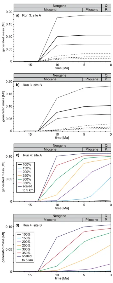
Petroleum system modelling conducted at two sites north of the ridge shows that the conditions for thermogenic methane production have been met in the area, which may have resulted in the production of up to 0.2 Mt of bulk petroleum in two potential phases since the early Eocene.

However, only the first phase in the early Eocene appears to be directly influenced by the thermal effects of the Knipovich Ridge. The second phase, which occurred in the Miocene, is mainly controlled by a rapid increase in sediment overburden.

The second study area on the Svalbard margin is located on the upper continental slope, where the base of the gas hydrate stability zone crops out at the seabed in water depths of <400 m. The zone of intersection is characterised by numerous gas flares, which have been interpreted to indicate the release of methane from gas hydrate dissociation in response to warming bottom waters. The article of Berndt et al. (2014b), to which I contributed as a co-author, supports the hypothesis of hydrate dissociation causing the observed fluid venting, but argues that the dissociation is due to seasonal variations of bottom-water temperatures, rather than caused by global ocean warming. A 2-year time series of bottom-water temperatures shows that temperatures reach peak values (up to 4.9°C) in autumn and winter and minimum values (0.6°C) in spring. Numerical modelling of the gas hydrate stability zone shows that these temperature fluctuations result in lateral shifts of the

(7)

v gas hydrate stability zone, which promote periodic dissociation and formation of hydrates near the zone of intersection. Carbonate samples from the seep sites indicate that seepage off Svalbard has been going on for several 1000 years.

Another study site is the Giant Gjallar Vent in the Norwegian Sea. The Giant Gjallar Vent is one of the largest vent systems in the North Atlantic and originated as a hydrothermal vent system at the Paleocene-Eocene transition. Previous studies based on 3D seismic data differed in their interpretations of the vent’s present activity, describing the system as buried or as recently reac- tivated. New high-resolution 2D seismic and sediment echosounder data are used to re-interpret the Quarternary activity of the Giant Gjallar Vent. The new data show that the up to 12 m high surface elevation of the vent is caused by up-doming of the Quarternary sediments, which represent a seal to upward fluid migration. The doming therefore occurs in response to the build-up of overpressure beneath the seal. At one location, the seal has been breached and a potential leakage pathway extends from the seal up to the seafloor. Although indications for active venting were not observed, it seems that the Giant Gjallar Vent is preparing for a new phase of venting activity.

The fourth studied fluid flow system consists of 25 cold seep sites on New Zealand’s Hikurangi Margin. The seeps exhibit various seabed morphologies that produce different intensity patterns in sidescan backscatter images. Classification of these patterns reveals that they fall into four distinct types that reflect variations in carbonate morphologies, including massive, up to 20-m-high structures (type 1), low-relief crusts (type 2), scattered blocks (type 3), and carbonate-free sites (type 4). The types correlate well with the occurrence of typical benthic seep fauna: communities living on sediment surfaces dominated at type 4 sites, seep fauna settling on hard substrate were found predominantly at type 2 and 3 sites, and non-seep epifauna were observed on type 1 carbonates of extinct cold seeps. Backscatter signatures in sidescan sonar images of cold seeps may therefore serve as a convenient proxy for variations in faunal habitats.

The studies show that all four fluid flow systems are unlikely to contribute significantly to the present climate warming period. Only two systems – the seeps on the upper slope off Svalbard and on the Hikurangi Margin – are actively releasing methane into the water column, but this release is not catastrophic. Rather, it is controlled by short-term variations in the fluid flow system, induced by changes in pressure and bottom-water temperature. However, gas hydrate systems and hydrothermal vent complexes must have contributed to climate warming in the past, e.g. during the Paleocene-Eocene Thermal Maximum. Quantification of the extent of these contributions should be the objective of future work.

(8)

Zusammenfassung

In Fluidflusssystemen werden methanangereicherte Fluide aus einem unterirdischen Reservoir durch die aufliegenden Sedimentschichten zum Meeresboden transportiert und dort ausgestoßen. Steigt das ausgestoßene Methan durch die Wassersäule bis an die Wasseroberfläche, tritt es in die At- mosphäre ein und kann somit zur Klimaerwärmung beitragen, denn Methan ist ein deutlich stär- keres Treibhausgas alsCO₂. Fluidflusssysteme, z.B. hydrothermale Schlote und Gashydratreser- voire, könnten in der Vergangenheit große Mengen Methan freigesetzt haben, welche zunächst in die Wassersäule und anschließend in die Atmosphäre gelangten. Es wird daher angenommen, dass Fluidflusssysteme einen wichtigen Beitrag zu großen Klimaerwärmungsereignissen wie dem Paläozän/Eozän-Temperaturmaximum leisteten. Das Ausmaß dieses Beitrages ist bislang jedoch nicht geklärt, weshalb detailliertere Studien zu Fluidflusssystemen erforderlich sind. In der vor- liegenden Arbeit werden vier Fluidflusssysteme bezüglich ihrer Entwicklung und ihrer Gasaus- trittsaktivität untersucht. Außerdem ist von Interesse, ob ein Zusammenhang mit der aktuellen Klimaerwärmungsphase sowie vergangenen Klimaereignissen besteht. Für die Untersuchungen wurden verschiedene geophysikalische Methoden wie 2D- und 3D-Seismik, Sidescan-Sonar- und Sedimentecholotmethoden eingesetzt, sowie Wärmeflussmessungen, geochemische Analyseverfah- ren und numerische Modellierung.

Die ersten beiden untersuchten Fluidflusssysteme befinden sich im Nordatlantik am Kontinental- rand von Spitzbergen. Diese Region zeichnet sich durch eine ausgedehnte Gashydratprovinz aus, die anhand sogenannter „bottom-simulating reflectors“ (bodensimulierende Reflektoren) in seismischen Daten nachgewiesen wurde. Die Verteilung der bodensimulierenden Reflektoren zeigt, dass sich die Gashydrate vor allem auf ein 3500 km² großes Gebiet nördlich des Knipovich-Rückens konzentrieren. Da der Knipovich-Rücken Teil des Mittelatlantischen Rückensystems ist, deutet dies darauf hin, dass vom Rücken ausgehende thermale Effekte zu thermogener Methanproduk- tion in der Nähe des Rückens führen könnten. Unterstützt wird diese Hypothese vom Wärmefluss, welcher vom Kontinentalrand bis zum Knipovich-Rücken deutlich zunimmt. Die an zwei Stellen nördlich des Rückens durchgeführte Petroleumsystemmodellierung zeigt, dass die für thermogene Methanproduktion nötigen Bedingungen erfüllt gewesen sein könnten. Dies könnte die Produk- tion von bis zu 0.2 Mt Petroleum (Öl und Gas) seit dem frühen Eozän ermöglicht haben, wobei die Produktion während zwei Phasen stattfand. Nur die erste dieser beiden Phasen, welche im frühen Eozän stattfand, scheint dabei direkt durch die thermalen Effekte des Knipovich-Rückens beeinflusst worden zu sein. Die zweite Phase, die sich im Miozän ereignete, wird hauptsächlich durch eine starke Zunahme der Sedimentauflast kontrolliert.

Das zweite Untersuchungsgebiet in der Region Spitzbergen befindet sich am oberen Hang des Kon- tinentalrandes, wo die Untergrenze der Gashydratstabilitätszone in einer Wassertiefe von <400 m den Meeresboden schneidet. Im Bereich des Zusammentreffens sind zahlreiche Gasfahnen zu beobachten, welche als Anzeichen für die Methanfreisetzung aus destabilisierenden Gashydraten

(9)

vii interpretiert werden. Es wird vermutet, dass die Gashydratauflösung durch sich erwärmendes Bo- denwasser verursacht wird. Der Artikel von Berndt et al. (2014), zu dem ich als Co-Autorin beigetragen habe, unterstützt die Hypothese der Gashydratdestabilisierung als Grund für die beobachte- ten Fluidaustritte. Jedoch scheint die Destabilisierung eher durch saisonale Schwankungen der Bo- denwassertemperatur bedingt zu sein, und nicht durch globale Ozeanerwärmung. Eine 2-Jahres- Zeitreihe der Bodenwassertemperaturen zeigt, dass die Temperaturen im Herbst bzw. Winter am höchsten sind (bis zu 4.9°C), während sie im Frühling ein Minimum erreichen (0.6°C). Die numerische Modellierung der Gashydratstabilitätszone verdeutlicht, dass die Temperaturschwankun- gen zu lateralen Verschiebungen der Gashydratstabilitätszone führen, welche periodische Destabili- sierung und Neubildung von Gashydrat zur Folge haben. Karbonatproben aus dem Bereich der Gasaustritte deuten an, dass Methanfreisetzung vor Spitzbergen schon seit mehreren 1000 Jahren geschieht.

Ein weiteres Untersuchungsgebiet ist der Giant Gjallar Vent in der Norwegischen See. Der Giant Gjallar Vent ist eines der größten Gasaustrittssysteme im Nordatlantik und entstand ursprünglich als Hydrothermalsystem während des Übergangs vom Paläozän zum Eozän. Frühere Studien sind unterschiedlicher Auffassung, was die derzeitige Aktivität des Gasaustrittssystems betrifft.

Anhand von 3D-seismischen Daten wurde der Giant Gjallar Vent entweder als inaktiv und ver- schüttet oder als kürzlich reaktiviert interpretiert. Neue, hochauflösende 2D-Seismik- und Sedi- mentecholotdaten erlauben nun eine Neuinterpretation der quartären Aktivität des Giant Gjallar Vents. Die Daten zeigen, dass die bis zu 12 m hohe Oberflächenerhebung über dem Aufstiegskanal durch Aufwölbung der quartären Sedimente verursacht wird, welche für aufsteigende Fluide weit- gehend undurchlässig sind. Die Aufwölbung ist bedingt durch die Akkumulation von Fluiden unterhalb der undurchlässigen Schicht und dem damit verbundenen Aufbau von Überdruck. An einer Stelle konnten die aufliegenden Sedimente jedoch durchbrochen werden und eine potentielle Leckagezone reicht bis zum Meeresboden. Zwar wurden keine Anzeichen für aktiven Fluidaustritt beobachtet, doch es scheint, als steuere der Giant Gjallar Vent auf eine neue Fluidaustrittsphase zu.

Das vierte untersuchte Fluidflusssystem besteht aus 25 Gasaustrittsstellen (sogenannten Cold Seeps) entlang des neuseeländischen Hikurangi-Kontinentalrandes. Die Austrittsstellen sind durch eine Reihe von Meeresbodenmorphologien gekennzeichnet, welche verschiedene Rückstreuungsmuster in Sidescan-Sonar-Daten produzieren. Die Klassifizierung dieser Muster zeigt, dass sich genau vier Mustertypen feststellen lassen. Die Mustertypen beschreiben Variationen der Karbonatmorpholo- gien und reichen von massiven, bis zu 20 m hohen Strukturen (Typ 1) über niedrige Krusten (Typ 2) und verstreute Blöcke (Typ 3) bis hin zu karbonatfreien Austrittsstellen (Typ 4). Die Muster- typen korrelieren gut mit der Verteilung typischer benthischer Meeresbodenfauna. So finden sich auf Sedimentoberflächen lebende Organismen an Typ-4-Stellen, während harte Oberflächen bevorzugende Fauna vor allem an Typ-2- und Typ-3-Stellen nachgewiesen wurde. Epifauna, welche nicht auf einen beständigen Methanfluss angewiesen ist, wurde auf Typ-1-Karbonaten inaktiver Austrittsstellen beobachtet. Rückstreuungsmuster in Sidescan-Sonar-Daten von Gasaustrittsstellen können somit wertvolle Hinweise auf Variationen in Meeresbodenhabitaten liefern.

Wie die vier Studien zeigen, ist es unwahrscheinlich, dass die untersuchten Fluidflusssysteme maß- geblich zur aktuellen Klimaerwärmung beitragen. Lediglich an zwei Systemen – die Gasaustritts-

(10)

stellen am oberen Kontinentalrand von Spitzbergen und am Hikurangi-Kontinentalrand – wird derzeit eine Freisetzung von Methan in die Wassersäule beobachtet. Diese Freisetzung ist nicht katastrophal, sondern wird stattdessen durch relativ kurzzeitige Variationen innerhalb des Fluid- flusssystems hervorgerufen. Dazu gehören beispielsweise Veränderungen im Druck und in der Bodenwassertemperatur. Trotzdem müssen Gashydratsysteme und hydrothermale Schlote in der Vergangenheit zu Klimaerwärmungsereignissen wie dem Paläozän/Eozän-Temperaturmaximum beigetragen haben. Die Quantifizierung dieser Beiträge bleibt das Ziel zukünftiger Forschung.

(11)

List of abbreviations

AOM anaerobic oxidation of methane BGHSZ base of the gas hydrate stability zone BPU Base Pleistocene Unconformity BSR bottom-simulating reflector

CMP common mid-point

CTD conductivity, temperature, density DSDP Deep Sea Drilling Project

GC gravity core

GGV Giant Gjallar Vent

GHSZ gas hydrate stability zone

HI hydrogen index

IODP Integrated Ocean Drilling Program

MASOX Monitoring Arctic Seafloor-Ocean Exchange mbsf metres below seafloor

mbsl metres below sea level

MC-ICP-MS multi-collector inductively-coupled plasma mass spectrometry

MCS multichannel seismic

MIC-ICP-MS multi-ion-counting inductively-coupled plasma mass spectrometry

MOx methane oxidation

ODP Ocean Drilling Program

PDB Pee Dee Belemnite

PETM Paleocene-Eocene Thermal Maximum

Q-ICP-MS quadrupole inductively-coupled plasma mass spectrometry SIRMS stable isotope ratio mass spectrometry

SMOW standard mean ocean water SMTZ sulphate-methane transition zone

TF transform fault

TOC total organic carbon

TWT two-way travel time

USBL ultra-short base line V-PDB Vienna Pee Dee Belemnite

XRD X-ray diffraction

xiii

(16)

(17)

Chapter 1

Introduction

The work presented in this thesis was carried out in the framework of the Kiel Cluster of Excellence

“Future Ocean”. The Cluster is a research network with members from the Christian-Albrechts- University in Kiel (CAU), the Helmholtz Centre for Ocean Research (GEOMAR), the Leibniz Institute for the World Economy (IfW), and the Muthesius Academy of Fine Arts and Design (MKHS). It is dedicated to the multidisciplinary study of the past and present ocean system and the application of these results to predict the future evolution of the world’s oceans.

The oceans strongly influence global climate and are vitally important for human welfare. How- ever, humans may also endanger the marine environment, and vice versa. For example, human actions such as pollution and anthropogenicCO₂emissions increasingly affect the oceans, whereas major natural hazards originating from the oceans, e.g. submarine landslides and tsunamis, present a risk to human life. It is therefore important to improve our understanding of the basic ocean system in order to better predict its reaction to changes and establish sustainable ocean management.

Future Ocean addresses these challenges in 11 research topics. This thesis is part of research topic R09, which investigates ocean controls on climate and environment at transitions to warming periods. More specific, R09 studies past events of climate warming to identify the main ocean feedback processes on climate, which will help to understand future global warming.

One aspect is to find out what role geological carbon emissions from fluid flow systems played in driving environmental change during warming periods such as the Paleocene-Eocene Thermal Maximum (PETM). Although fluid flow systems, where methane is transported from a subsurface reservoir to the seabed, have been extensively studied world-wide (e.g. Han and Suess, 1989;

Cartwright, 1994a; Pecher et al., 2004; Gay et al., 2007; Brothers et al., 2013), their contribution to the global carbon cycle is not well understood and often overlooked (Kvenvolden et al., 2001).

However, fluid flow systems may have released large amounts of methane into the water column and subsequently into the atmosphere (e.g. Dickens et al., 1995; Svensen et al., 2004). Methane that reaches the atmosphere can accelerate global warming, as it is a much stronger greenhouse gas thanCO2(Harvey and Huang, 1995). To understand how the oceans are dealing with large- scale methane input from fluid flow systems, and to constrain the geological forcing mechanisms of climate warming events such as the PETM, it is necessary to study these systems in more detail.

1

(18)

1.1 Fluid flow systems

Fluid flow systems are found in a variety of tectonic environments – active margins, passive margins, transform faults, and intraplate settings – and in all kinds of oceanographic settings, ranging from coastal areas to the deep ocean (e.g. Lewis and Marshall, 1996; Whiticar, 2002; Dupré et al, 2010; Gay et al., 2012; Talukder, 2012, and references therein; Leduc et al., 2013). There are many different types of fluid flow systems, such as hydrothermal vents (e.g. Jamtveit et al., 2004;

Planke et al., 2005), polygonal fault systems (e.g. Cartwright, 1994b; Berndt et al., 2003), and gas chimneys (e.g. Pecher et al., 2004; Løseth et al., 2009) (Fig. 1.1). Which type of fluid flow system is formed in an area depends not only on the tectonic setting and fluid composition, but especially on the processes driving fluid production and migration. Berndt (2005) distinguishes between compaction-controlled, volcanism-controlled, petroleum, and freshwater systems.

Despite the great variety of fluid flow systems, they usually have a common structure ( Judd and Hovland, 2007; Talukder, 2012). This structure consists of a fluid reservoir and a conduit for transporting fluids towards the seabed. In the case of active or past prolonged fluid venting, the systems are also often characterised by a surface expression ( Judd and Hovland, 2007; Talukder, 2012).

gas hydrate systems

tectonic faulting polygonal fault systems

hydrocarbon reservoir leakage

volcanic sill intrusions

rapid sedimentation

freshwater aquifers

pockmarks and cold seep ecosystems

pockmarks mud volcanoes

low permeability

low permeability low permeability

BSR

Figure 1.1: Illustration of different types of fluid flow systems that occur on passive continental margins. Most structures can also be found on active margins. Small filled circles represent gas bubbles. BSR – bottom-simulating reflector. (Berndt, 2005)

1.1.1 Fluid reservoirs

Fluids are stored in subsurface reservoirs. Reservoirs are generally zones of high porosity and permeability surrounded by sediments of lower permeability, or bounded by sealing faults ( Judd

(19)

1.1. FLUID FLOW SYSTEMS 3 and Hovland, 2007). Fluids are thus prevented from escaping. However, reservoir seals may become unstable and once leakage occurs, fluid flow systems may develop. Examples for reservoirs include deep (<1 km) hydrocarbon reservoirs (e.g. Gay et al., 2007), gas hydrate systems (e.g.

Kvenvolden, 1988), and shallow freshwater acquifers (e.g. Bokuniewicz, 1992) (Fig. 1.1).

1.1.1.1 Origin of gas

Most types of fluid flow systems are associated with methane, which is the most common gas in marine sediments ( Judd and Hovland, 2007). Sedimentary methane can be of either biogenic or abiogenic origin, with the term ‘biogenic’ referring to microbial (or bacterial) and thermogenic methane production (Whiticar, 1999).

Microbial methane

At least 20% of natural gas accumulations world-wide are associated with methane of microbial origin (Rice and Claypool, 1981; Wiese and Kvenvolden, 1993). Microbial methane is produced by methanogenic archaea during either CO₂ reduction in sulphate-free marine sediments (Equation 1.1), or acetate fermentation in freshwater sediments (Equation 1.2) (Whiticar et al., 1986; Schoell, 1988).

CO₂+ 4H₂ →CH₄+ 2H₂O (1.1)

CH3COOH→CH4+ CO2 (1.2)

Microbial methanogenesis in marine sediments requires anoxic conditions and temperatures of 4-55°C (optimum ∼35°C), although one species of methanogens can also exist at temperatures of up 97°C (Rice and Claypool, 1981; Wiese and Kvenvolden, 1993). Another requirement is the presence of organic matter (>0.5% total organic carbon (TOC)) (Rice and Claypool, 1981).

Large amounts of organic matter often accumulate in areas with high sediment input. However, sedimentation rates should not be too fast as burial also increases sediment temperature, which will cause methanogenesis to cease once the temperature window is exceeded. Clayton (1992) considers sedimentation rates of 200 to 1000 mMyr⁻¹ as optimal. Under favourable conditions, ∼10% of the TOC can be transformed into microbial methane (Clayton, 1992).

Thermogenic methane

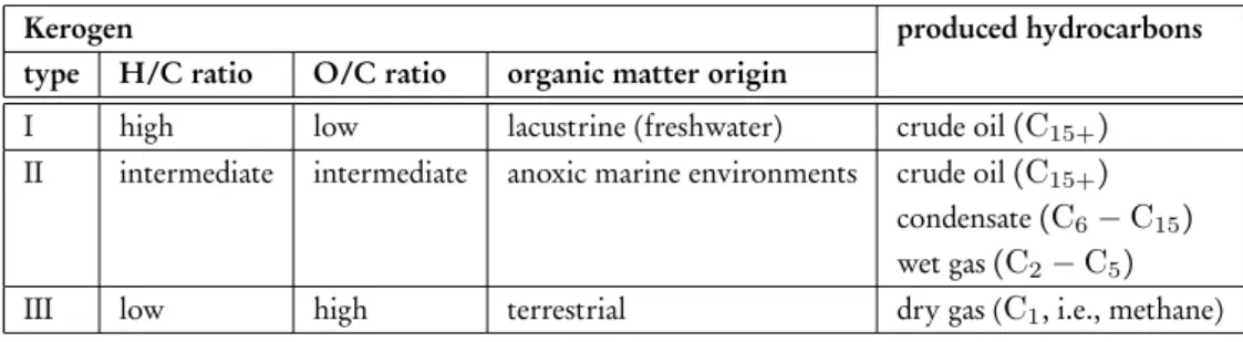
Organic matter that is not transformed remains in the sediment and eventually becomes kerogen, i.e., insoluble organic remains (Wiese and Kvenvolden, 1993). Sedimentary rocks that contain a high amount of kerogen (>2% TOC) are referred to as source rocks, from which hydrocarbons can be produced thermogenically ( Judd and Hovland, 2007). Thermogenic hydrocarbon production involves thermal cracking of kerogen. Depending on the type of kerogen, which is controlled by the H/C and O/C ratios, as well as the origin of the organic matter, different types of hydrocarbons are produced (Table 1.1) (Tissot and Welte, 1984).

(20)

Table 1.1: Overview of the different types of kerogen and associated hydrocarbons.

Kerogen produced hydrocarbons

type H/C ratio O/C ratio organic matter origin

I high low lacustrine (freshwater) crude oil(C15+)

II intermediate intermediate anoxic marine environments crude oil(C₁₅₊) condensate(C6−C15) wet gas(C2−C5)

III low high terrestrial dry gas (C1, i.e., methane)

In addition to the type of kerogen, the type of hydrocarbons produced also depends on the sediment temperature and the level of maturity (Wiese and Kvenvolden, 1993). Three levels of maturity are distinguished: (1) immature, where condictions for thermogenic hydrocarbon production are not yet fulfilled; (2) mature, i.e., production can take place; and (3) post-mature or overmature, where production is no longer possible. The temperature window for thermogenic hydrocarbon production is 60-260°C. Depending on the geothermal gradient, production may occur down to depths >10 km ( Judd and Hovland, 2007).

Abiogenic methane

Abiogenic methane, i.e., methane derived from inorganic processes, has been produced under lab- oratory conditions (Foustoukos and Seyfried, 2004), but conclusive evidence for its occurrence in natural settings is rare (e.g. Fiebig et al., 2009). Abiogenic methane production is proposed to occur at hydrothermal systems located either in sediment-free mid ocean ridge settings (Welhan, 1988) or onshore (Fiebig et al., 2009). In addition, abiogenic methane may form during serpentinization of the oceanic basement, e.g. at slow-spreading ridges (Minshull et al., 1998).

Distinguishing between origins of methane

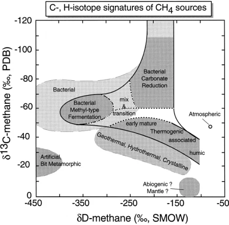
Stable isotope analysis is the most reliable tool to distinguish between different origins of methane (e.g. Rice and Claypool, 1981; Cicerone and Oremland, 1988). The method uses the ratio of the two stable carbon isotopes,¹³Cand¹²C, which differ strongly for the carbon of methane molecules of different origins. The isotope ratios are expressed in theδ¹³Cnotation (Equation 1.3) for which the Pee Dee Belemnite (PDB) standard is most commonly used.

δ¹³C = ¹³^C/¹²^C13^sampleC/¹²⁻C¹³standard^C/¹²^C^standard ×100 (1.3) Theδ¹³Cof methane is typically combined with the stable hydrogen isotope ratio δDas shown in Fig. 1.2. δD is based on the D/H ratio, or ²H/¹H, relative to the SMOW (standard mean ocean water) standard (Whiticar, 1999). Microbial methane is characterised byδ¹³Cvalues ranging between -110hto -50hand δD of -400hto -150h(Fig. 1.2). Thermogenic methane is more enriched in¹³C, resulting inδ¹³Cvalues of about -50hto -20h(Whiticar, 1999). Even heavier δ¹³Cvalues (>-20h) are associated with abiogenic methane (Fig. 1.2).

(21)

1.1. FLUID FLOW SYSTEMS 5

Figure 1.2: Diagram ofδ¹³CandδD, showing the classification of the different methane origins (bacterial, thermogenic, abiogenic). PDB – Pee Dee Belemnite, SMOW – standard mean ocean water. (Whiticar, 1999)

1.1.1.2 Gas hydrates

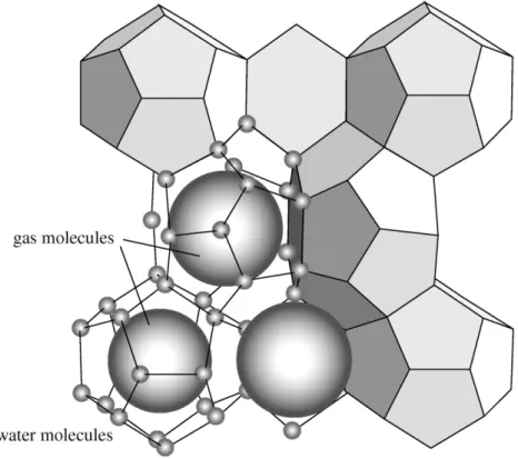
Gas hydrates are a subgroup of clathrates, i.e., solid compounds consisting of a guest molecule surrounded by a cage-like framework of molecules of a different kind (e.g. Pellenberg and Max, 2000). The guest molecule in hydrates is a gas molecule, typically methane, and the cage structure is made up of water molecules (Fig. 1.3) (Kvenvolden, 1993). Three types of hydrate structures (structures I, II, and H) are found in natural environments (Sloan, 1998). The structure determines how much methane gas can be contained in a certain amount of methane hydrate. For a fully saturated structure I hydrate - the most common structure in nature (Kvenvolden, 1995) - 1 m³ of methane hydrate may contain up to 164m³ of methane gas and 0.8m³ of water (Kvenvolden, 1993).

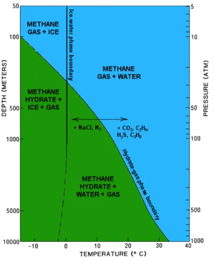
The stability of gas hydrates is strongly controlled by temperature and pressure conditions (Fig.

1.4). Gas hydrates are stable only at high pressures and low temperatures, which restricts their occurrence to areas characterised by water depths >300 m and bottom-water temperatures of less than 2°C (Kvenvolden, 1995). Gas hydrates are thus only found in onshore polar regions and deep marine environments such as continental slopes (Kvenvolden, 1993, 1995, 2000). In addition, gas hydrates can only form in areas with large supplies of water and gas molecules (Hovland and Judd, 1988).

(22)

In oceanic settings, gas hydrates are usually found at water depths exceeding 300-500 m (e.g. Hynd- man et al., 1992; Bouriak et al., 2000; Dillon and Max, 2000; Vanneste et al., 2005b; Haacke et al., 2007; Sarkar et al., 2012). Depending on the depth range of the gas hydrate stability zone (GHSZ), gas hydrates may be stable within the sediment as well as at and above the seabed. In general, the thickness of the GHSZ ranges between∼100 m and∼1 km (e.g. Chand et al., 2008) and is controlled by the geothermal gradient, the water temperature, the water depth (and hence pressure), the presence of inhibitors such as NaCl, and the gas composition (Sloan, 1998). The highest concentrations of hydrate are typically observed near the base of the gas hydrate stability zone (BGHSZ) (Dillon and Max, 2000).

Figure 1.3: Schematic of structure I gas hydrate. Water molecules form a cage structure that traps one gas molecule within it, e.g. methane. (Maslin et al., 2010)

More than 99% of the hydrate-bound gas molecules are typically methane (C1) with a δ¹³C between -57 to -73h, indicating microbial origin (Kvenvolden, 1995, 2000). However, hydrates may also contain higher hydrocarbons such as ethane (C₂) and propane (C₃). If more than 1% of higher hydrocarbons are present, this is a strong indication for the involvement of thermogenic gas. In fact, methane hydrates may hold a significant proportion of thermogenic methane, e.g. in the Gulf of Mexico (Brooks et al., 1986) and the Caspian Sea (Ginsburg et al., 1992).

Below the BGHSZ, free gas may exist, e.g. as a result of a temperature-induced vertical shift of the BGHSZ that caused hydrates at the bottom to be no longer stable (e.g. Dillon and Max, 2000).

Although hydrate-cemented sediments represent a barrier to upward gas migration, fluid pressures can become high enough to enable bypass of the GHSZ and subsequent migration towards the seabed (e.g. Gorman et al., 2002; Holbrook et al., 2002; Flemings et al., 2003; Tréhu et al., 2004).

(23)

1.1. FLUID FLOW SYSTEMS 7 Gas hydrates are thus important components in fluid flow systems as they represent reservoirs from which fluids may be transported upwards to be expelled at the seafloor.

Figure 1.4: Hydrate phase diagram illustrating the boundary between methane hydrate (green) and free gas (blue).

The addition of different molecules shifts the stability curve as indicated by the arrows. For the depth scale, lithostatic and hydrostatic pressure gradients of 10.1 kPam⁻¹are assumed. Adapted from Kvenvolden (1993).

1.1.2 Fluid conduits

Due to the low density of free gas, the reservoir fluids are buoyant and tend to migrate towards the seabed. Upward migration can also be promoted by overpressure, i.e., fluid pressure exceeding hydrostatic pressure (Clayton and Hay, 1994). However, capillary effects at pore throats may reduce the mobility of water-free gas mixtures (Clayton and Hay, 1994; Henry et al., 1999), and migration may be further impeded if the overlying sediment is resistant to fracturing (Clayton and Hay, 1994). Hyndman and Davis (1992) summarise three geological settings in which upward fluid migration commonly occurs: (1) accretionary wedges, where waterlogged sediments are com- pacted due to tectonic movements, (2) subduction zones, where accretionary wedges are absent but underthrusting of sediments occurs, and (3) passive-margin areas of rapid sediment loading.

Fluid migration is differentiated into primary migration, i.e., from the source rock to the reservoir, and subsequent secondary migration ( Judd and Hovland, 2007). Fluid transport towards the

(24)

seabed requires conduits linking the reservoir with the sediment surface. Such conduits are usually weakness zones that are either structurally or stratigraphically controlled (Krabbenhoeft et al., 2013).

Fluid flow patterns are often related to the presence of faults, as upward migration of fluids is facilitated by pre-existing fault networks, at least in the upper few 100 m (Clayton and Hay, 1994).

Where faults serve as migration conduits, fluid expulsion at the seafloor is often restricted to lo- calised zones (e.g. Barry et al., 1996; Stakes et al., 1999). Fluid flow to the seabed may continue as long as the fault network is kept open, e.g. by high pore fluid pressures. However, the closing of fault pathways will prevent further fluid migration and trap the fluids in the reservoir.

If a reservoir is effectively sealed and fluid accumulation continues, overpressure will build up due to the buoyancy of hydrocarbons (Osborne and Swarbrick, 1997). Once a critical threshold is reached, the reservoir seal will be fractured, allowing fluids to migrate into overlying sediments.

Fracturing of the seal occurs by either capillary failure when the capillary resistance to migration is exceeded, or fracture failure, where the overpressure is sufficient to induce fracturing (Clayton and Hay, 1994). New pathways are then opened, but previously closed fractures can also be re-used.

As the overpressure bleeds off, fractures will close again, which may result in periodic opening and closing of the seal in response to changing pore fluid pressures (Sibson et al., 1988; Cartwright, 1994a; Roberts and Nunn, 1995).

While vertical to near-vertical faults are the most common fluid migration pathways, lateral fluid advection is also observed (e.g. Stakes et al., 1999). In addition, fluid migration may be facilitated by permeable stratigraphic horizons and lenses, e.g. of sandy material. In this case, fluid pressures have to be sufficiently high to force a migration pathway (Clayton and Hay, 1994; Liu and Flemings, 2007).

1.1.3 Surface activity

Once migrating fluids reach the sediment surface, they are expelled into the water column. De- pending on the type of fluids, different terminology is used to describe the site of expulsion: “vents”

are associated with hydrothermal fluids, i.e., hot fluids, “seeps” refer to the venting of cold fluids, e.g. oil and gas, and “springs” occur where groundwater is expelled at the seafloor ( Judd and Hov- land, 2007). Prolonged fluid expulsion may affect the surrounding seabed, leading to a variety of seafloor features such as pockmarks, carbonate mounds, and mud volcanoes (e.g. Hovland and Judd, 1988).

1.1.3.1 Fluid venting

Activity of fluid venting may vary greatly, ranging from no activity at all to explosive fluid release.

Also, fluid venting is often not continuous but is rather characterised by periods of activity in- terrupted by times of quiescence. For example, durations of active emissions may vary between minutes to hours (e.g. Greinert et al., 2006; Krabbenhoeft et al., 2010). Leifer et al. (2004) compare

(25)

1.1. FLUID FLOW SYSTEMS 9 such episodic fluid release to an electrical circuit consisting of capacitors which need to recharge first before a new period of activity can begin.

Short-term variations of fluid venting activity have been associated with tidal influence (Greinert et al., 2006; Krabbenhoeft et al., 2010). During low tides, the pressure from the water column (the hydraulic head) is reduced, which facilitates upward fluid migration and thus leads to increased venting activity. Alternatively, pressure changes associated with ocean swells, storm surges, and biologic pumping could induce short-term fluid flow variations (Teichert et al., 2003).

On a larger time scale, periods of increased fluid release appear to be correlated with periods of sealevel low-stand during glacial cycles (e.g. Teichert et al., 2003; Kiel, 2009). The lower sealevel during glacial times causes the BGHSZ to shift to shallower levels, leading to increased gas hydrate decomposition and hence an increase in the amount of mobile fluids. Elevated fluid flux during glacial stages may also be due to increased sediment loading of continental slopes, which increases lithostatic pressure on source rocks and reservoirs, and hence subsurface overpressure (Kiel, 2009).

In addition, longterm variations of fluid venting activity can be related to tectonic processes such as earthquakes (Teichert et al., 2003). Over time, fluid venting may cease if fluid conduits are closed or the fluid reservoir becomes exhausted (Aharon et al., 1997).

The fate of methane bubbles released from seabed sources has been widely debated (e.g. Kven- volden et al., 2001; Leifer and Patro, 2002; MacDonald et al., 2002; Leifer et al., 2006; McGinnis et al., 2006). Methane bubbles emitted from seep sites ascend through the water column with rising speeds of around 10-30 cm s⁻¹ (MacDonald et al., 2002; Leifer and Judd, 2002; Greinert et al., 2006). The rising bubbles typically form a plume, which can be detected by hydracoustic systems (see 1.1.4). Such plumes may reach heights of up to 1300 m (Greinert et al., 2006) and, depending on the water depth, can thus effectively transport methane to the sea surface from where it will escape into the atmosphere.

The majority of methane, however, will be dissolved within the water column before it reaches the surface (e.g. McGinnis et al., 2006; Judd and Hovland, 2007; Schmale et al., 2010). Whether the methane bubbles survive the ascent through the water column depends on several factors, including water depth, bubble size, concentrations of dissolved gases, and temperature (Leifer and Patro, 2002). In addition, methane bubbles released from beneath the GHSZ are often protected by a hydrate coating that prevents early dissolution, thus increasing the likelihood of methane reaching the surface (Kvenvolden et al., 2001; Greinert et al., 2006; McGinnis et al., 2006). However, methane from seep sites is assumed to reach the surface only in shallow water areas (<100 m water depth) (McGinnis et al., 2006; Schmale et al., 2010), unless rapid upwelling flows are involved, which increase the rising speed of bubbles and could enable methane release from deeper (>250 m) waters (Leifer et al., 2006).

1.1.3.2 Cold seep systems

Cold seeps are associated with the expulsion of relatively cold fluids at the seabed. They occur in both active and passive margin settings and have been studied intensely under various geological, biological, physical, and chemical aspects (e.g. Talukder, 2012, and references therein). Their

(26)

occurrence indicates complex geological processes causing production, upward migration and subsequent seafloor venting of methane-rich fluids (Moore and Vrolijk, 1992; Judd and Hovland, 2007;

Talukder, 2012).

Cold seeps represent unique seafloor ecosystems that mainly originate from microbial activity.

Microbes settle in the shallow subsurface near the fluid pathways and, using sulphate as the oxidant, oxidise the supplied methane at the sulphate-methane transition zone (SMTZ), a process known as anaerobic oxidation of methane (AOM; Barnes and Goldberg, 1976) (Equation 1.4):

CH4+ SO⁻²₄ →HCO⁻₃ + HS⁻+ H2O (1.4)

AOM-performing microbial communities were first discovered by Boetius et al. (2000) at Hydrate Ridge on the Cascadia Margin. During AOM, hydrogen carbonate (HCO⁻₃) is produced, which decreases the pH and allows the precipitation of calcium carbonate (CaCO₃) from seawater.

Prolonged carbonate precipitation may lead to the formation of so-called chemoherms (Aharon 1994), i.e., seafloor carbonate structures of various morphologies. Authigenic carbonates also vary in dimensions, ranging from cm-scale carbonate cementations within the sediment (e.g. Ritger et al., 1987) over tubular structures (e.g. Stakes et al., 1999; Díaz-del-Río et al., 2003), massive blocks (e.g. Van Dover et al., 2003) and mounds (e.g. Klaucke et al., 2012) on the seafloor to steep pinnacles that have grown several tens of metres into the water column (Teichert et al., 2003).

Carbonate precipitates further differ in their chemical compositions, which reflect variations in the nature of the expelled fluids, the intensity of fluid flow, and local environment conditions during formation (e.g. Stakes et al., 1999; Liebetrau et al., 2010). Authigenic carbonates thus represent valuable archives in terms of past seep activity and the development of fluid systems.

Cold seep sites are important seafloor habitats as they are commonly inhabited by abundant benthic fauna that live on carbon-based chemosymbiosis (e.g. Barry et al., 1996; Sahling et al., 2002).

These include bacterial mats, vesicomyid clams, and ampharetic polychaetes at carbonate-free seepage locations, as well as mussels, siboglinid tubeworms, and sponges, which settle on the carbonate substrate of active seep sites (e.g. Barry et al., 1996; Lewis and Marshall, 1996; Sahling et al., 2002; Bowden et al., 2013). In addition, non-seep epifauna, e.g. cold-water corals, may grow on carbonate blocks after seepage ceased (Liebetrau et al., 2010; Bowden et al., 2013), e.g. through clogging of fluid pathways (Hovland, 2002). Consequently, the nature and abundance of biological communities at cold seep locations may give information on the activity of the fluid system.

1.1.4 Acoustic imaging of fluid flow systems

In acoustic records, fluid flow systems are generally identified from anomalies caused by the presence of free gas, either within the sediment or in the water column (e.g. Anderson and Bryant, 1990). Gas bubbles change the physical properties of sediments and water. In particular, they affect the impedance, i.e., the product of the acoustic velocity and the density of the medium (Sheriff and Geldart, 1995). The presence of gas bubbles thus results in a strong impedance contrast between gas-bearing and gas-free zones, which causes anomalies such as bright spots and hydroacoustic flares that are described below.

(27)

1.1. FLUID FLOW SYSTEMS 11 Acoustic energy that encounters a gas-bearing layer is scattered at the gas bubbles, and a higher proportion of the energy is reflected, inhibiting further penetration into the gas zone. Reflection is accompanied by phase reversal of the acoustic signal due to the negative reflection coefficient of gas (reverse polarity) (Sheriff and Geldart, 1995). Energy that is not reflected is attenuated, resulting in reduced penetration of the acoustic signal. The lower density associated with gas also causes a reduction in the P-wave velocity, whereas the S-wave velocity becomes zero as S-waves cannot travel through gas and liquids (Sheriff and Geldart, 1995).

The effect of gas on the acoustic signal strongly depends on the acoustic frequency and the size of the gas bubbles, which determines their resonance frequency. The strongest reaction is observed when the acoustic frequency is similar to the resonance frequency of the gas bubbles (Anderson and Bryant, 1990). High-frequency systems are generally more sensitive to gas. Consequently, acoustic anomalies caused by the same gas-bearing zone may vary significantly if acoustic systems of different frequencies are used.

The following list describes typical anomalies indicating the presence of gas bubbles:

• Hydroacoustic flares (Fig. 1.5A) are flare-shaped anomalies in the water column imaged by echosounder systems (e.g. Anderson and Bryant, 1990). They are caused by gas bubbles emanating from the seafloor at seep sites and indicate the scattering of acoustic energy in response to the impedance contrast between seawater and gas. Hydroacoustic flares can reach heights of several 100 m, with the highest (up to 1300 m) observed in the Black Sea (Greinert et al., 2006).

• Acoustic turbidityis the most common gas-related subsurface anomaly in acoustic records.

The term refers to chaotic low-amplitude reflections that occur in sediment echosounder data and high-resolution seismic data ( Judd and Hovland, 1992; Yuan et al., 1992; Whiticar, 2002).

Acoustic turbidity is caused by scattering and absorption of acoustic energy by gas bubbles and commonly obscures stratigraphic reflections. The effect is often observed underneath bright spots or enhanced reflections.

• Bright spots and enhanced reflectionsare high-amplitude reflections caused by the strong impedance contrast between a gas-free zone and a relatively thin gas-bearing zone within the sediment (e.g. Løseth et al., 2009). While enhanced reflections occur in shallow (<100 m) sediments and are therefore imaged by sediment echosounder systems, bright spots are observed below 100 m in seismic data (Hovland and Judd, 1988). Bright spots are often characterised by reverse polarity ( Judd and Hovland, 1992).

• Chimneys and pipes are vertical anomalies that indicate upward migration of free gas or gas-bearing fluids. Their generally low amplitude in both seismic and sediment echsounder data is caused by strong attenuation of the acoustic signal, but can also be due to the destruc- tion of the original sediment layering during migration processes (Hovland and Judd, 1988;

Schroot et al., 2005). Chimneys can have diameters of several 100 m (Fig. 1.5B) and are associated with relatively slow, upward gas migration via hydro-fracturing (Løseth et al., 2009).

(28)

Pipes often have smaller diameters (<300 m) and may also be characterised by stacked high- amplitude reflections (Fig. 1.5C) (Andresen et al., 2012). Unlike chimneys, pipes can form explosively, e.g. in response to a blow-out (Løseth et al., 2001, 2009). In the literature, the terms “chimney” and “pipe” are often used interchangeably to describe the same structures, as so far there is no clear distinction between the two types (Andresen et al., 2012).

• Down-bending reflections(pull-down) are observed in seismic and sediment echosounder data at the lateral transition between relatively gas-free and gas-bearing zones within the sediment (Hovland and Judd, 1988). The down-bending effect towards the gas-bearing zone is caused by the lower velocity in gas-charged sediments, which results in an increased travel time of the returned signal ( Judd and Hovland, 1992). This effect may also cause an apparent sagging of reflectors beneath a gas-bearing zone (e.g. Løseth et al., 2009).

• Up-bending reflections(pull-up) have been observed at the margins of chimney structures in seismic data (e.g. Hustoft et al., 2007, 2010; Westbrook et al., 2008b; Plaza-Faverola et al., 2011). They likely represent acoustic artefacts caused by higher-velocity material within the chimney. Gas hydrates within a chimney may cause P-wave velocities that are up to 300 ms⁻¹higher than in the surrounding sediments (Plaza-Faverola et al., 2010). Alternatively, higher velocities and associated up-bending reflections can be caused by carbonate cementing the chimney walls (e.g. Hustoft et al., 2007; Westbrook et al., 2008b).

Another type of acoustic anomaly is the bottom-simulating reflector (BSR) in seismic data. The BSR is characterised by a high-amplitude reflection that generally mimicks the seafloor and is of reverse polarity (Fig. 1.5D) (Shipley et al., 1979). The BSR is caused by the strong impedance contrast between stable gas hydrates above and free gas below (Shipley et al., 1979). Thus, the BSR does not only indicate the presence of gas hydrate but also marks the lower limit of the GHSZ. However, gas hydrates may also be present without a BSR being observed in seismic data (Holbrook et al., 1996; Haacke et al., 2007).

In addition to gas, seafloor carbonates also influence the returned acoustic energy. High-backscatter anomalies in sidescan sonar and multibeam backscatter data can indicate the presence of seep carbonates on the seabed (Fig. 1.5E) ( Johnson et al, 2003; Holland et al., 2006). The high backscatter results from (1) the difference in impedance contrast between carbonates and the surrounding seabed, (2) small-scale roughness of the carbonate surface, and (3) the morphology of the precipitates ( Johnson et al., 2003; Holland et al., 2006). However, if the seafloor around the carbonate structures is also highly reflective, e.g. due to rock outcrops or pronounced relief, the acoustic response of seep carbonates may be difficult to distinguish from the background backscatter.

(29)

1.1. FLUID FLOW SYSTEMS 13

E

D ^seafloor

polarity reversal across

BSR

slope2 length: 7.3 km gas-enhanced reflections with lower

frequency content Molloy

Transform

shot number

Two-way travel time [s]

seep carbonates ES60 (38 kHz)

A

5 minutes 800 m 700 m 600 m 500 m

flares

B C

gas chimney

pipe

BSR

Figure 1.5: Overview of different acoustic anomalies related to fluid flow. (A)Hydroacoustic flares in single-beam echosounder records from offshore New Zealand. Adapted from Greinert et al. (2010). (B)Seismic profile across the Tommeliten Alpha gas chimney in the North Sea. Adapted from Løseth et al. (2009). (C)Pipe structure offshore Namibia, imaged in seismic data. Adapted from Moss and Cartwright (2010). (D)Bottom-simulating reflector (BSR) imaged in seismic data from the western Svalbard margin. Adapted from Vanneste et al. (2005b).(E)High backscatter anomalies in sidescan sonar data indicating cold seep carbonates on the Chilean margin. Adapted from Klaucke et al.

(2012).

(30)

1.2 Motivation

Climate warming events have occurred several times throughout Earth’s history. Major events took place at the late Permian–Triassic boundary (∼253 Ma) (Wignall, 2001; Retallack and Jahren, 2008), in the early Jurassic (Toarcian;∼183 Ma) (Hesselbo et al., 2000; Svensen et al., 2007), and at the Paleocene-Eocene transition (PETM;∼55 Ma) (Dickens et al., 1995; Dickens, 1999). All three events were characterised by an abrupt increase in atmospheric methane concentration and a disturbance of the global carbon cycle, which has been attributed to the sudden release of large amounts of methane gas into the atmosphere (e.g. Dickens et al., 1995; Hesselbo et al., 2000;

Svensen et al., 2004).

The best studied climate warming event is the PETM, which was characterised by an increase in bottom-water temperatures of at least 4°C (Dickens et al., 1995; Dickens, 1999). At the same time, carbon isotope data show an anomaly of -2 to -3hin the δ¹³C of the ocean-atmosphere system (Dickens et al., 1995). This anomaly indicates a rapid injection of isotopically light carbon (¹²C) into the oceans and atmosphere (Dickens, 1999; Röhl et al., 2007). Although the PETM lasted about 170 ka (Röhl et al., 2007), two thirds of the carbon were probably injected over a time span of only a few thousand years, indicating catastrophic carbon release (Norris and Röhl, 1999). Such rapid carbon injection requires an extensive reservoir capable of releasing large amounts of carbon over a short time span (Dickens, 1999). Several studies (e.g. Dickens et al., 1995; Norris and Röhl, 1999; Maclennan and Jones, 2006) agree that gas hydrate systems could constitute such a reservoir.

Methane release from gas hydrates, i.e., hydrate dissociation, occurs in response to changes in temperature and/or pressure that result in hydrates being no longer stable (Fig. 1.6) (e.g. Kvenvolden, 1988; Dillon and Max, 2000). Hydrate dissociation is observed today in several areas, e.g. on the Cascadia margin (Suess et al., 1999), the Norwegian margin (Mienert and Posewang, 1999; Jung and Vogt, 2004), the Svalbard margin (Westbrook et al., 2009; Berndt et al., 2014b), the U.S. Atlantic (Phrampus and Hornbach, 2012; Phrampus et al., 2014) and Pacific margins (Hill et al., 2004), and even in lacustrine settings such as Lake Baikal (van Rensbergen et al., 2003). The consequences of large-scale hydrate dissociation include ocean acidification, enhanced dewatering of marine sediments, sediment mobilisation, turnover of benthic material, and methane plumes extending into the water column and potentially reaching the atmosphere (Suess et al., 1999; Vogt and Jung, 2002;

van Rensbergen et al., 2003; Biastoch et al., 2011; Reagan et al., 2011). Methane that reaches the atmosphere may contribute to a positive climate feedback as it can accelerate the warming process (e.g. Harvey and Huang, 1995).

An increase in bottom-water temperature would mostly affect shallow gas hydrate deposits, whereas deep-ocean hydrates would remain stable (Reagan and Moridis, 2007, 2008). Reagan and Moridis (2008) estimate that a 1°C temperature increase could already result in the release of substantial amounts of methane gas from shallow gas hydrates. A 3°C increase may even cause destabilisa- tion of∼85% of the global methane hydrate deposits (Buffett and Archer, 2004). For the PETM,

(31)

1.2. MOTIVATION 15 the 4°C increase in bottom-water temperature and subsequent hydrate dissociation are thought to have resulted in the release of about 1000-2000 Gt of carbon enriched in¹²C(Dickens et al., 1995;

Dickens 1999). According to Dickens et al. (1995) and Dickens (1999), such quantities would be sufficient to explain theδ¹³Canomaly.

gas released by dissociating hydrate old base of GHSZ

migrating gas

fractures as water temperature rises,

GHSZ moves down slope old top

of GHSZ

plumes of gas bubbles sea surface

hydrate seabed

?

Figure 1.6: Hydrate dissociation caused by changing bottom-water temperatures. An increase in bottom-water temperature causes the GHSZ to move downslope, resulting in the dissociation of hydrates to methane gas and water. The released gas is free to move to the seabed where it escapes into the water column and possibly the atmosphere. Redrawn after Westbrook et al. (2009).

In addition, hydrate dissociation may also be caused by tectonic uplift as this results in depressurisation. Depressurisation can cause hydrates to become unstable even if bottom-water temperatures remain constant (Sloan, 1998). Maclennan and Jones (2006) propose that regional uplift occurred at the onset of the PETM and may thus have contributed to carbon release from destabilising methane hydrates.

In order to assess which areas are most vulnerable to large-scale hydrate dissociation and methane release under warming conditions, knowledge of the amount and distribution of hydrates in marine sediments is required. One approach is numerical modelling, which takes into account the deposition and degradation of organic matter, burial history, and bottom-water temperatures. The resulting estimates of the global amount of carbon stored in methane hydrates vary between 3-455 Gt (Piñero et al., 2013),>455 Gt (Wallmann et al., 2012), 4-995 Gt (Burwicz et al., 2011), 500-2500 Gt (Milkov, 2004), 1146 Gt (Kretschmer et al., submitted), and 1600-2000 Gt (Archer et al., 2009).

Buffett and Archer (2004) estimated a total of 5000 Gt of which 3000 Gt are stored in hydrates and 2000 Gt in free methane bubbles.

(32)

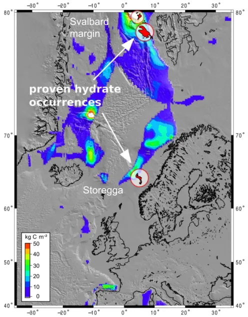
Numerical modelling provides a good overview of the areas where hydrates would be stable, which are generally restricted to continental slope and shelf regions (Maslin et al., 2010, and references therein). An alternative method to assess hydrate distribution is the mapping of the BSR, which requires seismic data and can therefore only be applied in regional studies. This approach is more precise than numerical modelling but may result in a minimum hydrate distribution, as gas hydrates do not always cause a BSR in seismic data (Holbrook et al., 1996; Haacke et al., 2007).

Svalbard margin

Storegga

50 40 30 20 10 0 kg C m ²^-

Figure 1.7: Predicted distribution of gas hydrates based on global models (Kretschmer et al., submitted). Colours denote the amount of carbon stored in hydrates in mass per area. The predicted hydrate distribution is overlain with the distribution of actually observed hydrates based on the seismic BSR and drill cores (red areas).

Comparison of the two approaches shows that their results may differ significantly, e.g. in the North Atlantic (Fig. 1.7). While numerical modelling suggests that most of the eastern North Atlantic margin is within the zone of gas hydrate stability (Kretschmer et al., submitted), seismic BSRs indicate the presence of hydrates in only two comparatively small areas: on the western Svalbard margin (e.g. Vanneste et al., 2005a, 2005b; Bünz et al., 2008, 2012) and at the headwall

(33)

1.2. MOTIVATION 17 of the Storegga Slide (e.g. Mienert et al., 1998; Bünz et al., 2003, 2004, 2005). Even if taken into account that the absence of a BSR does not necessarily rule out the presence of hydrates (Holbrook et al., 1996; Haacke et al., 2007), the mismatch between areas of predicted and BSR-derived hydrate occurrence is obvious. This suggests that model-based estimations of the amount of carbon stored in hydrates may be overestimations that do not reflect actual observations.

If the real amount of hydrate-bound carbon is considerably smaller than that estimated from models, the amount of carbon released during warming-induced hydrate dissociation would also be smaller than estimated, and may thus not be sufficient to explain the carbon anomaly associated with the PETM. This is supported by Higgins and Schrag (2006), who believe that hydrate dissociation alone is insufficient to explain the substantial carbon addition to the atmosphere. Conse- quently, to assess the causes of methane release during climate warming events, it is also necessary to take into account other possible contributors.

Several other potential contributors to catastrophic methane release have been discussed, including thawing of permafrost soils (e.g. Schuur et al., 2009), burning peatlands (Higgins and Schrag, 2006) and a bolide impact (Cramer and Kent, 2005). The most likely contributor, however, are hydrothermal vent systems that result from magmatic intrusions into organic-rich sediments (Svensen et al., 2004). Contact metamorphism around the intrusions produces large amounts of thermogenic methane, promoting the development of fluid pipes and explosive fluid venting (Fig. 1.8) ( Jamtveit et al., 2004; Svensen et al., 2004; Planke et al., 2005; Aarnes et al., 2010). Although the venting activity following the intrusion emplacement is relatively short-lived (10-1000 years;

Svensen et al., 2004; Aarnes et al., 2010), the pipe structures may be re-used at later times (Svensen et al., 2003; Planke et al., 2005).

Both types of fluid flow systems that represent potential main contributors to climate warming events – gas hydrate systems and hydrothermal vent complexes – can be studied in the North At- lantic, which is also most sensitive to climate warming effects (Spielhagen et al., 2011). On the Svalbard margin, a large gas hydrate system extends from the continental slope to the Mid Atlantic Ridge system (Vanneste et al., 2005a, 2005b; Bünz et al., 2008, 2012; Hustoft et al., 2009). The presence of extensive gas hydrates could be related to methane production influenced by the proximity of active spreading ridges such as the Knipovich Ridge, as the associated high heat flow could promote thermogenic methane production (Vanneste et al., 2005a; Smith et al., 2014). On the upper slope, the BGHSZ crops out at the seafloor in water depths of less than 400 m (Westbrook et al., 2009). This zone is therefore most vulnerable with respect to an increase in bottom-water temperature. Over the past 30 years, bottom-water temperatures off Svalbard have increased by 0.3-2.0°C (Schauer et al., 2008; Ferré et al., 2012), and the observation of more than 250 gas flares at the intersection of the BGHSZ and the seafloor has been attributed to hydrate dissociation caused by a downslope retreat of the BGHSZ in response to higher bottom-water temperatures (Westbrook et al., 2009).

Further south, on the Norwegian margin, an 80,000 km² large sill complex was emplaced at the Paleocene-Eocene transition during the opening of the North Atlantic. The sill intrusion was associated with explosive methane venting and the formation of at least 2000-3000 hydrothermal vent complexes in the Vøring and Møre basins (Svensen et al., 2004; Planke et al., 2005). A total

(34)

of 734 vent complexes have so far been identified on seismic data (Svensen et al., 2004; Planke et al., 2005). One of these is the Giant Gjallar Vent (Gay et al., 2012), which is one of the largest fluid escape structures found in the North Atlantic. Although two large pipe structures indicate fluid migration activity long after the initial hydrothermal system formed, opinions on the present activity status differ, suggesting either reactivation (Gay et al., 2012) or extinction (Hansen et al., 2005).

Figure 1.8: Schematic illustrating the formation of a hydrothermal vent complex. (A)During sill intrusion, boiling pore fluids and gas formed due to metamorphic reactions cause a build-up of fluid pressure and explosive formation of a cone-shaped hydrothermal complex. The initial fluid expulsion is short-lived (10-1000 years) and associated with the generation of hydrothermal breccias.(B)Later, smaller pipes may develop within the cone structure, cross-cutting the breccias and enabling renewed fluid venting. ( Jamtveit et al., 2004; Planke et al., 2005)

1.3 Study objectives

The overall aim of this thesis is to better understand fluid flow systems in terms of past and ongoing activity, and their impact on oceans and the atmosphere. In particular, it is of interest if such systems may have contributed significantly to climate warming events such as the PETM.

In this thesis, four fluid flow systems are studied through a variety of geophysical methods, ranging from reflection seismic and hydroacoustic (Parasound, sidescan sonar, multibeam echosounder) methods to numerical modelling. The fluid flow systems are in different stages of development with respect to the classic fluid flow system structure described in 1.1. They also differ in their tectonic settings, which include both active and passive margins. Study areas are the western Svalbard margin, where two locations are studied – the area north of the Knipovich Ridge and the upper continental slope –, as well as the Giant Gjallar Vent in the Norwegian Sea and the Hikurangi Margin offshore New Zealand.

(35)

1.4. THESIS OUTLINE 19 The main questions posed for each study area are:

Svalbard margin – Knipovich Ridge

• Did the Knipovich Ridge influence petroleum generation on the Svalbard margin?

• What is/are the source(s) of fluids in this area?

Svalbard margin – seeps on upper slope

• What is the role of short-term variability of bottom-water temperatures for seepage at the BGHSZ seafloor intersection off Svalbard?

• What is the minimum age for the onset of marine methane release from the seafloor?

Giant Gjallar Vent (GGV)

• Is the GGV still active or does the observed surface relief reflect past activity of a now inactive system?

• Can the GGV be used as a study site for constraining the geological processes that are or were active in the deep part of the Vøring Basin?

Hikurangi Margin

• How do surface expressions of cold seeps differ in terms of backscatter intensity in sidescan sonar images?

• Can sidescan sonar data be used as a proxy for faunal habitats?

1.4 Thesis outline

This thesis consists of an introductory chapter (Chapter 1), followed by four case studies that describe fluid flow systems in different stages of development (Chapters 2-5), and a concluding chapter (Chapter 6). The case studies represent stand-alone manuscripts with their own abstract, introduction, methods, results, discussion, and conclusion sections. They have either been published by or will be submitted to international peer-reviewed journals.

Chapter 2 presents a fluid flow system early in its development, located north of the Knipovich Ridge on the western Svalbard margin. Gas hydrates in this region are more widespread than anywhere else in the eastern North Atlantic, indicating a substantial gas reservoir. The origin