1
Uncertainty in 21st Century Projections of the Atlantic Meridional Overturning 1
Circulation in CMIP3 and CMIP5 models 2
3
A. Reintges (corresponding author), T. Martin, M. Latif 4
GEOMAR Helmholtz Centre for Ocean Research Kiel 5
Düsternbrooker Weg 20, 24105 Kiel, Kiel, Germany 6
e-mail: areintges@geomar.de 7
telephone: +49 431 600-4007 8
fax: +49 431 600-4052 9
10
N. S. Keenlyside 11
Geophysical Institute and Bjerknes Centre, University of Bergen 12
Allégaten 70, 5020 Bergen, Norway 13
14 15 16 17 18 19 20 21 22
NOTE: This is a post-peer-review, pre-copyedit version of an article published in Climate 23
Dynamics. The final authenticated version is available online at:
24
https://link.springer.com/article/10.1007/s00382-016-3180-x 25
Please cite as Reintges, A., Martin, T., Latif, M. and Keenlyside, N. S. (2017) Uncertainty in 26
twenty-first century projections of the Atlantic Meridional Overturning Circulation in CMIP3 27
and CMIP5 models. Climate Dynamics 49:1495-1511. doi:10.1007/s00382-016-3180-x 28
2
Uncertainty in 21st Century Projections of the Atlantic Meridional Overturning 29
Circulation in CMIP3 and CMIP5 models 30
Annika Reintges, Thomas Martin, Mojib Latifand Noel S. Keenlyside 31
Abstract 32
Uncertainty in the strength of the Atlantic Meridional Overturning Circulation (AMOC) is 33
analyzed in the Coupled Model Intercomparison Phase 3 (CMIP3) and Phase 5 (CMIP5) 34
projections for the 21st century; and the different sources of uncertainty (scenario, internal and 35
model) are quantified. Although the uncertainty in future projections of the AMOC index at 36
30°N is larger in CMIP5 than in CMIP3, the signal-to-noise ratio is comparable during the 37
second half of the century and even larger in CMIP5 during the first half. This is due to a 38
stronger AMOC reduction in CMIP5. At lead times longer than a few decades, model 39
uncertainty dominates uncertainty in future projections of AMOC strengthin both the CMIP3 40
and CMIP5 model ensembles. Internal variability significantly contributes only during the first 41
few decades, while scenario uncertainty is relatively small at all lead times. Model uncertainty 42
in future changes in AMOC strength arises mostly from uncertainty in density, as uncertainty 43
arising from wind stress (Ekman transport) is negligible. Finally, the uncertainty in changes in 44
the density originates mostly from the simulation of salinity, rather than temperature. High- 45
latitude freshwater flux and the subpolar gyre projections were also analyzed, because these 46
quantities are thought to play an important role for the future AMOC. The freshwater input in 47
high latitudes is projected to increase and the subpolar gyre is projected to weaken. Both the 48
freshening and the gyre weakening likely influence the AMOC by causing anomalous salinity 49
advection into the regions of deep water formation. While the high model uncertainty in both 50
parameters may explain the uncertainty in the AMOC projection, deeper insight into the 51
mechanisms for AMOC is required to reach a more quantitative conclusion.
52
3
Keywords: Atlantic Meridional Overturning Circulation (AMOC), North Atlantic ocean, 53
uncertainty, climate projections 54
55
1. Introduction 56
The AMOC (Ganachaud and Wunsch 2003; Srokosz et al. 2012) is characterized by a 57
northward flow of warm, salty water in the upper layers of the Atlantic, and a southward return 58
flow of colder water in the deep Atlantic (Dickson and Brown 1994). It transports a substantial 59
amount of heat from the tropics and Southern Hemisphere toward the North Atlantic, where the 60
heat is then transferred to the atmosphere. The mild climate of Northern Europe is in part a 61
consequence of this heat supply. Changes in the AMOC are thought to have a profound impact 62
on many aspects of the global climate system. For example, the Atlantic Multidecadal 63
Oscillation or Variability (AMO/V), a coherent pattern of multidecadal variability in surface 64
temperature centered on the North Atlantic Ocean, is linked to the AMOC in climate models 65
(Knight et al. 2005; Zhang and Delworth 2006). Further aspects that are hypothesized to be 66
related to the AMOC are: observed decadal variability in the air-sea heat exchange over the 67
North Atlantic (Gulev et al. 2013), continental summertime climate of both North America and 68
western Europe (Sutton and Hodson 2005), Atlantic hurricane activity, Sahel rainfall and the 69
Indian Summer Monsoon (Zhang and Delworth 2006).
70
Direct measurements of AMOC strength from the RAPID-MOCHA array at 26.5°N reveal a 71
decline since 2004 (McCarthy et al. 2012, Smeed et al. 2014): During 2008-2012 the AMOC 72
was 2.7 Sv (1 Sv = 106 m³/s) weaker than during 2004-2008. Because of the relatively short 73
observational record it is unclear whether this decline is just a short-term fluctuation or part of 74
a long-term trend. However, records show that density in the Labrador Sea began to fall in the 75
late 1990s, and this may suggest more persistent AMOC weakening (Robson et al. 2014).
76
4
Roberts et al. (2014) suggest that this decline could be due to internal variability. However, 77
they also stress that the CMIP5 models generally underestimate the interannual variability of 78
the AMOC. This may be also the case at decadal timescales due to salinity biases, as recently 79
discussed by Park et al. (2016).
80
How will the AMOC evolve during the next decades and the whole 21st century? Future changes 81
in the AMOC will result from both internal and external processes of the climate system. On 82
the one hand, in control integrations with fixed external forcing many climate models simulate 83
strong internal AMOC variability on decadal to multi-decadal and even centennial timescales 84
(e.g., Danabasoglu 2008; Latif et al. 2004; Knight et al. 2005; Park and Latif 2008;Delworth 85
and Zeng 2012; see Latif and Keenlyside 2011 for a review). On the other hand, external forcing 86
such as anthropogenic emissions of long-lived greenhouse gases (GHGs) driving global 87
warming may also influence the future AMOC, as has been shown in numerous modeling 88
studies. The internal decadal to centennial AMOC variability will superimpose and hinder 89
detection of a potential anthropogenic AMOC signal, which evolves on similar timescales.
90
A wide variety of mechanisms have been put forward for how global warming will influence 91
AMOC. Global warming in response to enhanced atmospheric GHG concentrations will be 92
accompanied by changes in the vertical temperature and salinity profiles in the ocean. The 93
meridional structure of these changes will affect the meridional oceanic density contrast, which 94
has been suggested to be correlated with the AMOC strength (e.g., Thorpe et al. 2001).
95
Additionally to the importance of these processes, a large number of theoretical and modeling 96
studies pointed out the control of the AMOC by a number of internal ocean processes (as 97
reviewed by Kuhlbrodt et al., 2007). Delworth et al. (1993) suggested an interdecadal 98
oscillation caused by the interaction between the AMOC and the horizontal gyre circulation.
99
The influence of the subpolar gyre on the AMOC was supported by a multi-model study of Ba 100
et al. (2014). Further, a remote influx at the depth of the overturning, due to changes in the 101
5
Southern Ocean wind stress and Antarctic Bottom Water (AABW) formation, might counteract 102
the effect of changes in the meridional density gradient (de Boer et al. 2010). Shakespeare and 103
Hogg (2012) found that the AMOC scales linearly with both the Southern Ocean wind stress 104
and northern buoyancy flux. Gnanadesikan (1999) pointed out that the difference between 105
northern sinking and upwelling in the Southern Ocean are balanced by changes in the low- 106
latitude isopycnal depth. The rate of sinking in the north depends on the parameterization of 107
vertical mixing. Sijp et al. (2006) derived the importance of isopycnal mixing in models, 108
because it does not require a strong vertical instability. They argue that buoyancy-driven 109
convection overestimates the sensitivity of deep water production against surface freshwater 110
fluxes. The temporal and spatial interactions of all these processes determine the mean state, 111
the internal variability and the externally caused changes of the AMOC intensity. Finally, the 112
relative importance of these processes is unknown under changing climate conditions, and 113
might be different from the importance of the processes that determine the mean state in climate 114
model projections. Thus there are major uncertainties in how AMOC will respond to global 115
warming.
116
Climate models generally predict a weakening of the AMOC during the 21st century when 117
forced by enhanced levels of GHG concentrations, but large uncertainties exist (e.g., Schmittner 118
et al. 2005). This uncertainty can be conceptually decomposed into three components (Hawkins 119
and Sutton 2009, Hawkins and Sutton 2011): First, the future GHG emissions are unknown.
120
The climate models are therefore run under different GHG scenarios, leading to the so-called 121
scenario uncertainty. Second, a large uncertainty exists, even under identical GHG forcing 122
(Schmittner et al. 2005). One reason for this uncertainty is internal stochastically driven AMOC 123
fluctuations (e.g., Park and Latif 2012, Mecking et al. 2014). This kind of uncertainty is called 124
internal variability. Third, there is uncertainty arising from model systematic error that is called 125
model uncertainty, also sometimes termed response uncertainty. Model uncertainty might 126
6
originate from the ocean, the atmospheric or the sea ice components of the coupled models, 127
since all three influence the surface fluxes of heat, freshwater and momentum that drive the 128
AMOC. For example, the large mean biases in the North Atlantic found in the most climate 129
models (Wang et al. 2014) lead to errors in the northward path of saline waters, potentially 130
affecting internal variability and the model response to enhanced GHG concentrations.
131
The main purpose of this study is to investigate the consistency between the CMIP models with 132
regard to projecting 21st century GHG-forced AMOC change and to identify the origin of 133
uncertainties. As the complex processes controlling AMOC are poorly understood, a full 134
mechanistic understanding of future projections in AMOC remains a major challenge in climate 135
research and is beyond the scope of this paper. The focus of this paper is rather to examine a 136
few key variables that have been identified to be of relevance for the AMOC. We follow the 137
methodology outlined by Hawkins and Sutton (2009) and quantify as function of lead time the 138
three individual contributions – scenario, internal, and model – to the total AMOC projection 139
uncertainty. We show that, in both the CMIP3 and CMIP5 model ensembles, model uncertainty 140
dominates AMOC projections for the 21st century at lead times beyond a few decades. This 141
paper is organized as follows. In Section 2, we describe the data and the methodology used in 142
this study. We present the results of the AMOC projection uncertainty analysis in Section 3.
143
The results are summarized in Section 4.
144
2. Data and methodology 145
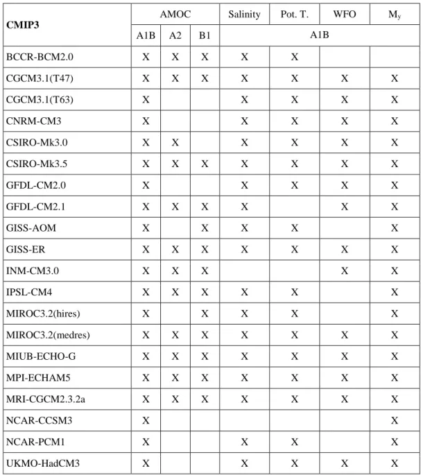
Data 146
We have used climate model simulations from the World Climate Research Programme’s 147
(WCRP’s) Coupled Model Intercomparison Project phase 3 (CMIP3; Table 1) (Meehl et al.
148
2007a) and phase 5 (CMIP5; Table 2) (Taylor et al. 2012). The multi-model datasets are 149
provided by the Program for Climate Model Diagnosis and Intercomparison (PCMDI). From 150
7
CMIP3 we used the 20C3M data for the 20th century and the IPCC SRES scenarios A1B, A2, 151
and B1 for the 21st century. The scenario B1 comprises the weakest, A1B a moderate, and A2 152
the strongest radiative forcing. For the CMIP5 analysis, we used the ‘historical’ data 153
representing the 20th century and the RCP4.5 and RCP8.5 scenarios for the 21st century. These 154
two scenarios are core experiments of CMIP5, and thus were performed with virtually all 155
participating models. The scenario with higher radiative forcing is RCP8.5. Combining the 156
20th– and the 21st-century scenarios our analysis covers the period 1850-2100. The CMIP 157
models provide the depth profile of the meridional overturning streamfunction in the Atlantic, 158
defined in z-coordinates and as function of latitude. From this variable we also computed the 159
indices of the AMOC strength by taking the maximum in the vertical for a given latitude. This 160
is a common measure of the AMOC strength. In the CMIP3 ensemble, the mean depth of the 161
overturning streamfunction maximum at 30°N during the years 1970-2000 is 1,115 m with an 162
inter-model standard deviation of 519 m and in the CMIP5 ensemble, 1,036 m with an inter- 163
model standard deviation of 140 m. These numbers seem to be reasonable when compared to 164
the observed profile at 26°N which also depicts a maximum at roughly 1,100 m (Smeed et al.
165
2014). For our analysis we use the latitudes 30°N and 48°N, because in most models 30°N 166
matches the center of the overturning cell quite well, whereas 48°N is a location with large 167
variability. Furthermore, zonal mean salinity and potential temperature profiles are analyzed in 168
this study. These were also used to calculate density changes. We also investigate the Arctic 169
and North Atlantic freshwater fluxes (WFO) from 0°-90°N integrated over different areas.
170
WFO includes the effects of evaporation, precipitation, river runoff, and sea ice changes.
171
Finally, we compute the uncertainties also for the subpolar gyre index, which is derived from 172
the barotropic streamfunction.
173
For most of the variables, we perform most of our analysis separately on both CMIP3 and 174
CMIP5 data. The total number of models in the CMIP3 database is smaller than that of CMIP5 175
8
(Tables 1 and 2). Of course, the models are not entirely independent of each other; some models 176
originate from the same modeling center and some share the same model components (Masson 177
and Knutti 2011). Therefore, the model uncertainty derived from the model ensemble used here 178
could be biased. To test this, we repeated the analyses with a smaller ensemble by removing 179
those models that have a setting too close to another model or behave too similar regarding one 180
or more variables. Our main findings remained qualitatively unchanged in these tests. Finally, 181
one should note that the forcing used in the CMIP3 and CMIP5 integrations is similar but not 182
identical; this is discussed below in the result section.
183
Statistical method 184
Uncertainty is a term used in different fields. In this study, uncertainty reflects the spread 185
between ensemble members within the CMIP projection of future climate. The CMIP data offer 186
a wide range of results for historic simulations and future climate projections. As the true path 187
of AMOC strength is unknown, it is difficult to evaluate the quality of the model-based future 188
projections. To define uncertainty we derive variances from inter-simulation differences. Total 189
uncertainty may not be decomposed into a linear combination of individual sources of 190
uncertainty, as cross terms may exist (i.e., variance of one component might depend on one of 191
the other factors). For example, the sensitivity to a specified forcing scenario and the internal 192
variability could be related and be model-dependent. However, here we are not interested in the 193
uncertainty of individual model projections, but only in integral quantities computed over the 194
complete model ensemble. Furthermore, we analyzed the cross terms and found them to be 195
sufficiently small not to impact the major conclusions of this work, and thus they will be 196
neglected in the remainder of the analysis.
197
For the quantification of the three sources of uncertainty we basically follow the approach 198
suggested by Hawkins and Sutton (2009), although we adapted the method for calculating the 199
internal variability. A more complete framework has been proposed, but it was shown to give 200
9
similar results when analyzing CMIP3 models (Yip et al. 2011). For a given scalar variable of 201
our analysis (e.g. AMOC strength or density at a fixed position) we define the term model 202
projections X(m,s,t) as the climate realizations dependent on time, t, and obtained from various 203
CMIP models, m, and different 21st century forcing scenarios, s. The projections X(m,s,t) are 204
split into a long-term variability component, representing the response to external forcing 205
Xf(m,s,t), and a short-term residual ε(m,s,t), representing internal fluctuations:
206
X(m,s,t) = Xf(m,s,t) + ε(m,s,t) (1).
207
A model response to external forcing is typically computed as the mean across a large ensemble 208
of experiments performed with that model prescribing identical external forcing but started 209
from different initial conditions. In the absence of such data we estimate the external forced 210
AMOC component, Xf(m,s,t), by a 4th order polynomial fit computed over the full time series.
211
A 4th-order polynomial is chosen as it captures the non-linear response of AMOC to external 212
forcing that includes the reduced weakening of the AMOC at the end of the 21st century found 213
in several models. Our main conclusions remain insensitive to this choice, as shown by 214
repeating the uncertainty analysis of the AMOC index at 30°N from the CMIP5 ensemble with 215
polynomial orders from 2, 3, and 5 (see supplementary material).
216
Then, from the long-term fit Xf(m,s,t) we calculate a long-term anomaly xf(m,s,t) relative to the 217
initial value i(m,s), which is the average over the years 1970 to 2000:
218
Xf(m,s,t) = i(m,s) + xf(m,s,t) (2).
219
Three sources of uncertainty are distinguished. The calculation of these components involves 220
taking the variance over the respective component. In our equations, we use a variance operator 221
defined as follows:
222
𝑉𝐴𝑅𝑑(𝑝) = 1
𝑁𝑑− 1 ∑ (𝑝 − 1 𝑁𝑑∑ 𝑝
𝑑
)
2
(3).
𝑑
223
10
Here, p is any parameter for which the variance is computed in the dimension d.
224
The first source of uncertainty is the internal variability and defined as 225
𝐼 = 1
𝑁𝑠∑ 1 𝑁𝑚
𝑠
∑ 𝑉𝐴𝑅𝑡
𝑚
(𝜀(𝑚, 𝑠, 𝑡)) (4).
226
Ns and Nm are the numbers of scenarios and models, respectively. Internal variability is 227
represented by the variance of the residual ε(m,s,t) over time, averaged over all models and all 228
scenarios. Therefore, internal variability is given as one value.
229
The second source of uncertainty is the model uncertainty and defined as 230
𝑀(𝑡) = 1
𝑁𝑠∑ 𝑉𝐴𝑅𝑚(
𝑠
𝑥𝑓(𝑚, 𝑠, 𝑡)) (5).
231
It represents the spread between the different model realizations. Here, we take the variance of 232
the long-term anomaly xf(m,s,t) over the model dimension m, and then average over the different 233
scenarios. According to our definition the internal variability includes only frequencies on inter- 234
annual or decadal timescales. Since the AMOC exhibits long-term variability (e.g. the Atlantic 235
Multidecadal Variability, AMV), which cannot be completely filtered out by the polynomial 236
fit, the model uncertainty contains also some uncertainty due to internal variability.
237
The third source of uncertainty is the scenario uncertainty and defined as 238
𝑆(𝑡) = 𝑉𝐴𝑅𝑠 ( 1
𝑁𝑚∑ 𝑥𝑓(𝑚, 𝑠, 𝑡)
𝑚
) (6).
239
It represents the spread of the long-term anomaly xf(m,s,t), averaged over all models for each 240
scenario. The estimate of the total uncertainty T(t) is defined as the sum of the internal, model 241
and scenario uncertainty. Finally, we calculated the signal-to-noise ratio SNR(t) with a two- 242
sided confidence level c:
243
11 SNR(t) = 𝐺(𝑡)
𝑞𝑐 2
√𝑇(𝑡) (7).
244
Here 𝑞𝑐
2
is the 𝑐
2
th quantile of the standard normal distribution. In this analysis, a confidence 245
level of 90% is used. G(t) is the mean signal 246
𝐺(𝑡) = 1
𝑁𝑠∑ 1 𝑁𝑚
𝑠
∑ 𝑥𝑓(𝑚, 𝑠, 𝑡)
𝑚
(8) 247
which is estimated from the averaged model fit xf considering all models and scenarios. A 248
signal-to-noise ratio SNR(t) larger than unity indicates that the mean climate signal G(t) exceeds 249
the amplitude of the noise and is therefore detectable. The uncertainty analysis below is based 250
on decadal means.
251
3. Results 252
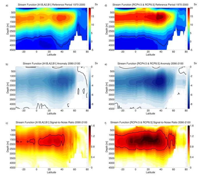
AMOC 253
The ensemble-mean of the late 20th century (1970-2000) Atlantic meridional overturning 254
streamfunction depicts a distinct maximum just below 1000 m in the region 30°N-45°N in both 255
the CMIP3 (Fig. 1a) and CMIP5 (Fig. 1d) model ensemble. The North Atlantic Deep Water 256
(NADW) cell reaches down to roughly 3000 m, which is shallower than what observations 257
suggest (McCarthy et al. 2012). We note, however, that the vertical extent of the cell varies 258
from model to model. The overall structure of the ensemble-mean is rather similar in the two 259
CMIP ensembles, but the mean strength of the overturning is considerably stronger in the 260
CMIP5 ensemble. The vertical maximum at 26°N is close to 19 Sv in the CMIP5 ensemble, as 261
opposed to 16 Sv in the CMIP3 ensemble. These numbers are closer to the observations 262
obtained from the RAPID array at 26°N, indicating AMOC strength of about 17.5 Sv during 263
the years 2004-2012 (Smeed et al. 2014). Decadal variability, however, may be large.
264
Furthermore, it must be noted that the spread among the models is huge and for the vertical 265
12
maximum at 26°N the models provide a range of 12.1 - 29.7 Sv in CMIP5 and 6.6 – 27.4 Sv in 266
CMIP3. The ensemble-mean AABW cell, which is located below the NADW cell, is rather 267
similar in both ensembles.
268
The ensemble-mean projected change in the Atlantic meridional overturning streamfunction for 269
the end of the 21st century (2090-2100 relative to 1970-2000) is shown in Fig. 1b and 1e. A 270
clear weakening of the NADW cell is seen in both ensembles, with the strongest change in the 271
streamfunction near 40°N, while there is a slight strengthening of the AABW cell. The spatial 272
pattern of the change is rather similar, but the magnitude is considerably stronger in the CMIP5 273
ensemble. In both ensembles, the maximum reduction occurs below the absolute maximum of 274
the ensemble-mean streamfunction, which results in a shallower NADW cell. We note that 275
although the radiative forcing is roughly comparable in the two ensembles, it is not identical.
276
For example, the changes in global annual-mean surface air temperature by the year 2100 277
depending on the scenario are: in CMIP3 1.8°C (B1), 2.8°C (A1B), 3.6°C (A2) relative to 1980- 278
1999 (Meehl et al. 2007b); and in CMIP5 1.9°C (RCP4.5), 4.1°C (RCP8.5) relative to 1986- 279
2005 (Collins et al. 20013). The relative change of the overturning is comparable and amounts 280
to about a 25-30% reduction by the end of the 21st century. The stronger absolute weakening in 281
the CMIP5 ensemble causes a larger signal-to-noise ratio in the CMIP5 ensemble with a 282
maximum of about 1.5 (Fig. 1f) as opposed to about 1 in the CMIP3 ensemble (Fig. 1c). A 283
signal-to-noise ratio of unity denotes the significance limit with 90%-confidence. Thus, a value 284
of 1.5 is indicative of a highly significant and detectable change.
285
In the following, we take the maxima of the streamfunction at 30°N and 48°N as indices for the 286
AMOC strength. The 30°N index is close to the center of the overturning cell and also is a good 287
indicator for a large meridional scale of the cell. Additionally, we select an AMOC index at 288
48°N that is close to the northern edge of the overturning cell and displays higher variability 289
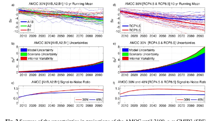
than the index at 30°N. We show the individual projections at 30°N for both CMIP3 (Fig. 2a) 290
13
and CMIP5 (Fig. 2d), for each model and for each scenario, with a 10-year running mean 291
applied to aid visualization (but all uncertainty analysis is performed on decadal means). A 292
large spread is obvious in the long-term AMOC projections at 30°N in the CMIP3 and CMIP5 293
ensembles. In both ensembles, the largest contribution to the total uncertainty is related to the 294
model differences (blue) at almost all lead times (Fig. 2b, 2e); while the contribution from the 295
internal variability (red) is rather small at all lead times. Although climate models may 296
underestimate the interannual variability of the AMOC (Roberts et al. 2014), model uncertainty 297
would still dominate by far even if the internal variability component was twice as large as 298
estimated here. Similarly, model uncertainty dominates for any reasonable choice of 299
polynomial order used to identify the forced component (see supplementary material). By 2100, 300
the contribution of scenario uncertainty (green) is substantial (about 20%) in the CMIP5 301
ensemble, but is rather small in the CMIP3 ensemble. This may be partly related to the larger 302
range of radiative forcing and to larger model sensitivity in CMIP5. Independently of this, the 303
main conclusion is unchanged as we move from CMIP3 to CMIP5: the model uncertainty is by 304
far the largest contribution to the total uncertainty in the AMOC projections for the 21st century 305
at lead times of several decades and beyond. Both CMIP ensembles yield a relatively large 306
signal-to-noise ratio for the AMOC change at 30°N (red line in Fig. 2c and 2f) at lead times 307
beyond a few decades. The signal-to-noise ratio tends to diminish at longer lead times. This 308
reflects the dominance of the model uncertainty compared to the projected AMOC reduction.
309
The signal-to-noise ratio is generally larger at 30°N than at 48°N (blue line in Fig. 2c and 2f), 310
which indicates a greater detectability of an anthropogenic signal in the subtropics compared to 311
the mid-latitudes.
312
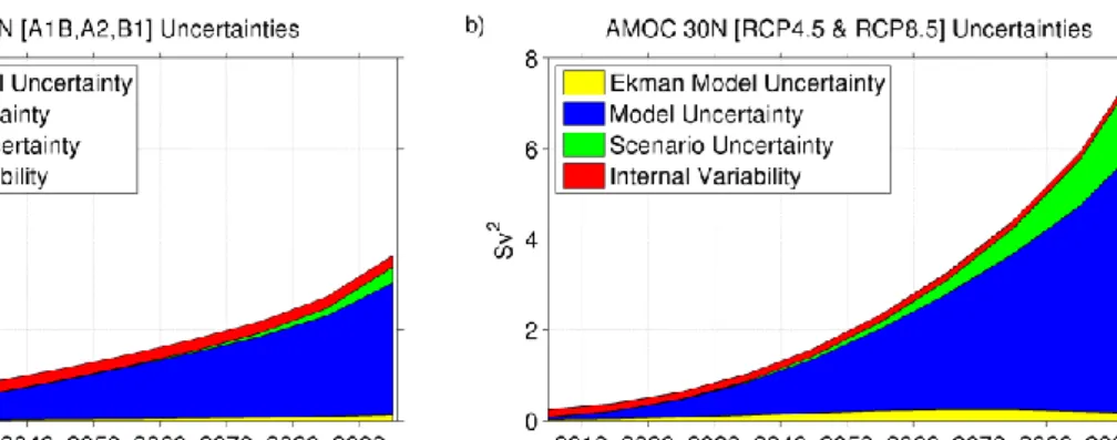
Although geostrophic transport dominates the time-mean AMOC, both geostrophic and Ekman 313
transports are important in explaining the AMOC variability. We derived the Ekman 314
contribution to the AMOC model uncertainty at 30°N from the wind stress curl field (Visbeck 315
14
et al. 2003). The Ekman component of model uncertainty is shown together with the remaining 316
model uncertainty and the other two uncertainty sources in Fig. 3. The Ekman contribution 317
(yellow) is rather small and becomes comparable to the AMOC uncertainty due to the internal 318
variability by the end of the 21st century. The Ekman uncertainty is thus, in both model 319
ensembles, only a marginal contributor to the total AMOC projection uncertainty.
320
As scenario uncertainty plays only a minor role compared to model uncertainty, we will focus 321
on only one scenario per model ensemble during all following analyses. We choose scenarios 322
with a moderate radiative forcing: SRES A1B for CMIP3 and RCP4.5 for CMIP5. One should 323
keep in mind that the global-mean surface air temperature change by the year 2100 is larger in 324
A1B (2.8°C relative to 1980-1999) than in RCP4.5 (1.9°C relative to 1986-2005).
325
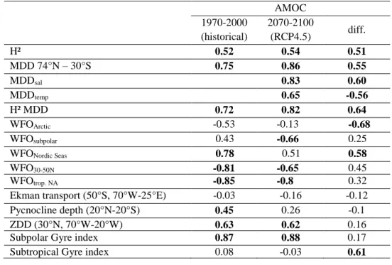
We benchmark the relationships of the AMOC to several parameters that have been previously 326
identified as relevant, for both CMIP3 and CMIP5 ensembles as follows: Table 3 lists 327
correlations computed across the model ensembles between the AMOC index at 30°N and these 328
parameters (see table caption for definitions). For the correlations time averages over 1970- 329
2000 or 2070-2100 are used. The correlations are not computed in the time- but in the model- 330
domain (detailed equations are given in the supplementary material). We use all available 331
models for these correlations. We did not remove outliers because there are no uniform metrics 332
that define an outlier reliably. Sometimes one model seems to perform well for one variable but 333
not for a different one. The strongest and significant correlation with the mean AMOC index at 334
30°N in the model ensemble for both periods is found for the subpolar gyre (SPG) index (rhistorical
335
= 0.87 and rRCP4.5 = 0.88). The SPG index is defined here as the minimum of the barotropic 336
streamfunction in the region 60°W-15°W / 45°N-65°N, and multiplied by -1. The SPG mean 337
state is negative in the barotropic streamfuction, indicating anti-clockwise circulation, and our 338
SPG index hence reflects the strength of this anti-clockwise circulation. Also the Atlantic mean 339
meridional depth-integrated density difference (MDD) is significantly related to the AMOC 340
15
index (rhistorical = 0.75 and rRCP4.5 = 0.86). A separation of MDD into salinity- and temperature- 341
driven components (MDDsal and MDDtemp) suggests that salinity dominates this relationship, 342
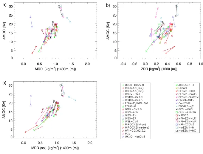
especially when the correlation of the differences is compared. Scatter plots between the AMOC 343
index and density gradients from the CMIP3 and CMIP5 models (Fig. 4) show that a strong 344
AMOC goes along with a large meridional density gradient. This relationship is in agreement 345
with studies that incorporate simple box models of the Stommel type (Stommel 1961).
346
However, we want to stress that the variability of the AMOC and general ocean circulation in 347
a climate model is driven by more complex ocean-atmosphere interactions. The near-linear 348
relationship between the AMOC index and the meridional density gradient (Fig. 4a) is primarily 349
caused by the changes in salinity (Fig. 4c). Due to geostrophy, we also expect a dependence of 350
the AMOC strength on the zonal density gradient (Sijp et al. 2012). However, the link between 351
the AMOC index and the zonal density difference (ZDD) is weaker (rhistorical = 0.63 and rRCP4.5
352
= 0.62; Fig. 4b) than the link to MDD, and changes in ZDD are only weakly related to projected 353
changes in AMOC strength (r=0.16). Further parameters that exhibit no strong correlation to 354
the AMOC index are the northward Ekman transport at the southern border of the Atlantic 355
(50°S) and the pycnocline depth.
356
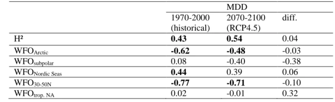
As MDD appears to be closely related to the projected AMOC changes, a similar correlation 357
analysis was performed to identify the factors most related to the MDD (Table 4). The 358
freshwater flux at the ocean surface (WFO) seems to play a role in determining the mean 359
meridional density gradient. We also considered integrating the freshwater flux over time for 360
this analysis. However, this did not affect the relative importance of model uncertainty and 361
internal variability, nor the signal-to-noise ratio. We find negative correlations with WFOArctic
362
(integrated over the Arctic; rhistorical = -0.62 and rRCP4.5 = -0.48) and WFO30-50N (integrated over 363
the Atlantic 30°-50°N; rhistorical = -0.77 and rRCP4.5 = -0.71). But for the difference between the 364
two periods there is no relationship (rdiff. = -0.03 / -0.10). We point out that the validity of our 365
16
results in Tables 3 and 4 is limited. Low correlations with the AMOC index may be biased by 366
strong model uncertainties. For example, the weak link of the ZDD with AMOC does not 367
necessarily imply that the former is unrelated to AMOC strength or change. Instead, this may 368
reflect differences in model dynamics. Furthermore, correlation analysis cannot identify causal 369
links. However, in the following we will place emphasis on parameters with a high correlation 370
to the AMOC strength or with the AMOC changes.
371
Density structure 372
All processes maintaining the density distribution in the water column are potentially important 373
in steering the AMOC. Although virtually all models simulate a significant weakening of the 374
AMOC under global warming conditions (Fig. 2), the reasons for changes and resulting 375
feedback mechanisms in the individual models may differ, which is eventually reflected in a 376
large model spread. In the 20th century runs, the simulated spatial and temporal distribution of 377
the modeled temperature and salinity fields largely differ from model to model. Furthermore as 378
mentioned above, the models suffer from large biases (e.g., Schneider et al. 2007).
379
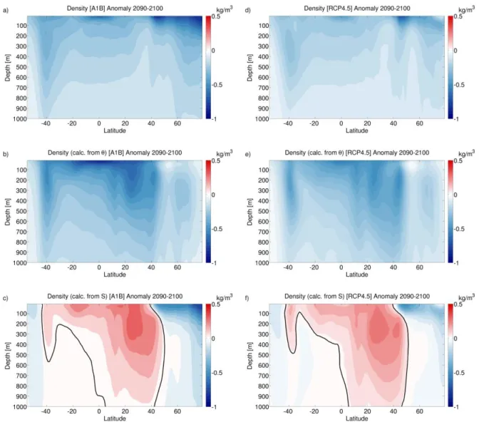
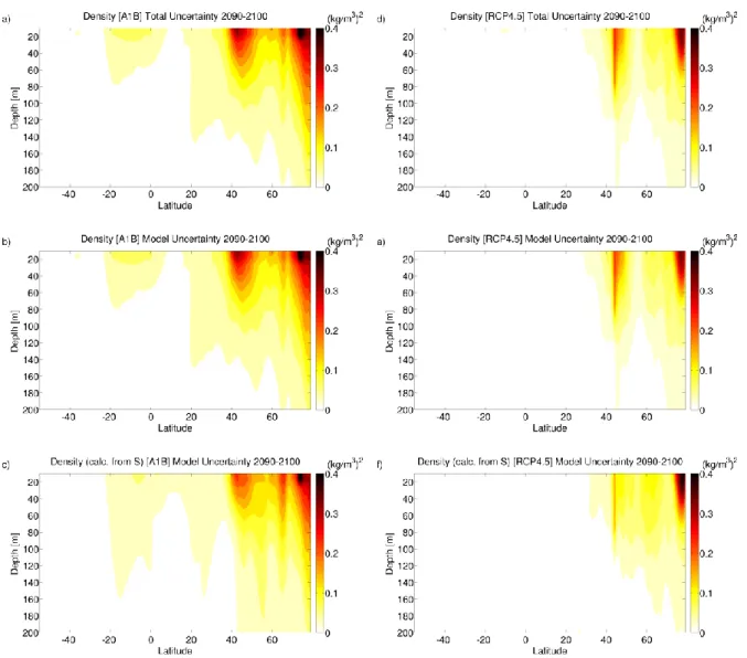
The CMIP3 A1B (Fig 5a) and CMIP5 RCP4.5 (Fig. 5d) ensemble-mean projected changes in 380
density, averaged zonally across the Atlantic, both show a strong reduction at the ocean surface, 381
generally weakening with depth. The strongest surface density reduction occurs north of 40°N, 382
with a secondary minimum near the Equator. The density signal penetrates relatively deep into 383
the Arctic Ocean. In the Southern Hemisphere mid-latitudes near 45°S, the mean profiles show 384
a strongly reduced density of the water column down to 1000 m depth. For some depth levels 385
in CMIP5 RCP4.5, the Southern Hemisphere decrease in density is even larger than in the 386
Arctic.
387
The impact on the density field through changes in temperature and salinity changes are also 388
separated. The temperature effect dominates in the tropics and subtropics (Fig. 5b and 5e), 389
17
where it strongly reduces the density. Salinity on the other hand tends to enhance the density 390
(Fig. 5c and 5f). A very strong salinity-induced increase in density is located around 30°N 391
extending to a depth of about 1000 m. At higher latitudes, especially in the Arctic region, the 392
models consistently project a strong salinity-induced reduction in density within the upper 1000 393
m. The pattern in the salinity contribution to the density change might lead to an intensified 394
meridional freshwater transport from the subtropics to the mid- and high latitudes, especially in 395
the Northern Hemisphere. Enhanced sea ice melt and stronger river runoff into the subpolar 396
North Atlantic and into the Arctic basin are also important in this context.
397
The largest uncertainties in the CMIP3 A1B projections of the density profiles (Fig. 6a and 6d) 398
are located in the mid-latitude North Atlantic and Arctic with largest values close to the surface.
399
Clearly, the overwhelming contribution to the total uncertainty in the projected density 400
originates from the model uncertainty (Fig. 6b and 6e). By separating the model uncertainty in 401
the density projections into a thermal- and a saline-driven part, it becomes also clear that the 402
latter explains the major fraction of the model uncertainty, especially in the Arctic (Fig. 6c and 403
6f). The results concerning the density changes from CMIP3 are basically confirmed by those 404
from CMIP5, with the caveat that the changes in CMIP5 tend to be somewhat weaker. Some of 405
this difference could be due to weaker radiative forcing of the RCP4.5 scenario used in CMIP5 406
compared to the A1B scenario in CMIP3.
407
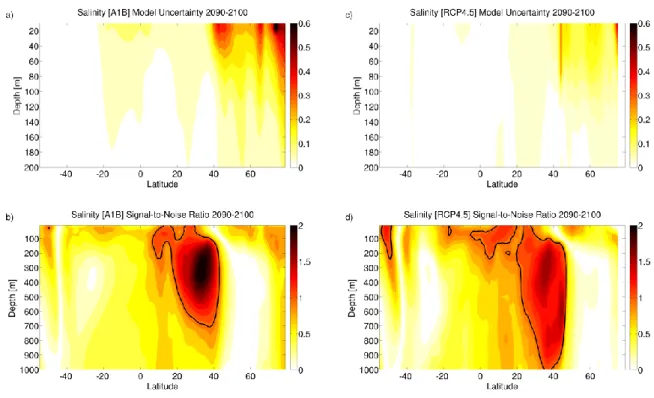
We now turn to the salinity projections themselves. The model uncertainty and the signal-to- 408
noise ratios for both the CMIP3 and CMIP5 ensembles are estimated using the A1B and RCP4.5 409
scenarios (Fig. 7). Consistent with the salinity contribution to the density uncertainty (Fig. 6c 410
and 6f), the uncertainty in the salinity projections obtained from CMIP3 shows the largest 411
uncertainties in the mid-latitude North Atlantic and in the Arctic (Fig. 7a and 7c). The 412
uncertainty of the salinity projections obtained from the CMIP5 ensemble is much reduced 413
compared to that calculated from the CMIP3 models. In the CMIP3 ensemble, a well distinct 414
18
region of high signal-to-noise ratio in the salinity projections is located in the region 20°N- 415
40°N within the upper 700 m centered at a depth of about 300 m (Fig 7b). In the CMIP5 416
ensemble, a similar pattern is found (Fig. 7d). However, the maximum values of the signal-to- 417
noise ratio are somewhat smaller than in CMIP3. Still, the area where it exceeds unity is larger 418
than in CMIP3. A gain in confidence is seen in a narrow region around 40°N below 700 m.
419
Further regions of enhanced signal-to-noise ratio in CMIP5 are found in the Southern 420
Hemisphere at 0°-20°S and south of 40°S, approximately in the upper 200 m.We conclude that 421
the model uncertainty determines the uncertainty in the density projections by the end of the 422
21st century, and that the uncertainty in the salinity projections is most relevant to the 423
uncertainty in the density projections. In this study, we focus on the spread of model projections.
424
Our results by no means imply that temperature changes are unimportant for the future 425
evolution of the AMOC, but they appear to play a secondary role for the model uncertainty.
426
Freshwater budget 427
We next investigate the projections for the freshwater flux integrated over the Arctic 428
(WFOArctic). In the CMIP5 ensemble, the projected changes in WFOArctic are anti-correlated with 429
the changes in the AMOC index at 30°N (Table 3: rdiff = -0.68). The projected mean WFOArctic
430
features some “outliers”, which does not allow drawing reliable conclusions. There also is a 431
strong anti-correlation between mean WFOArctic and the meridional density gradient (Table 4:
432
rhistorical = -0.62 and rRCP4.5 = -0.48). The projections of WFOArctic under the A1B (CMIP3) and 433
RCP4.5 (CMIP5) scenarios both show a negative ensemble-mean trend (Fig. 8a and 8d), which 434
leads to a freshening of the Arctic. However, the spread among individual models is large. In 435
the CMIP5 projections (Fig. 8e), the model uncertainty is remarkably reduced compared to 436
CMIP3 (Fig. 8b). This improvement could be caused by the higher complexity of the CMIP5 437
models that among others employ higher resolution. As a consequence, small-scale processes 438
influencing evaporation, precipitation, river runoff, and/or sea ice can be more realistically 439
19
simulated. Consistent with this, the signal-to-noise ratio (Fig. 8c and 8f) is larger in CMIP5, but 440
it does not exceed 1.2. Uncertainty in freshwater flux affects the surface salinity in the Arctic 441
and also remote regions by advection. The large uncertainty in surface salinity north of 40°N 442
(Fig. 7) is at least partially explained by the highly uncertain freshwater budget. However, the 443
projected changes in WFOArctic and in MDD (for 2070-2100 relative to 1970-2000) are not 444
significantly correlated in the CMIP5 ensemble (Table 4: rdiff. = -0.03), underscoring the 445
complexity of freshwater processes in the climate models.
446
Subpolar Gyre index 447
Our results suggest that the processes in the northern North Atlantic are most important for the 448
model uncertainties in the AMOC. This is equally confirmed by both CMIP3 and CMIP5.
449
Therefore, our following analysis on the subpolar gyre (SPG) index is only based on the CMIP5 450
model ensemble. The models project an ensemble-mean reduction in the SPG index until 2100 451
in both scenarios (RCP4.5 and RCP8.5). The SPG index during the reference period (1970- 452
2000) is 42.3 Sv, with a projected weakening until 2090-2100 of 10.6 Sv in RCP4.5 and 13.8 453
Sv in RCP8.5, i.e. a reduction of about 25% and 33%, respectively. The SPG and the AMOC 454
indices are highly correlated across the model ensemble (Table 3: rhistorical = 0.87 and rRCP4.5 = 455
0.88). However, the correlation between the projected changes of these two periods is weak 456
(rdiff. = 0.17). The large model spread of the SPG projection (Fig. 9a) results in high model 457
uncertainty, which is much higher than the internal variability and scenario uncertainty (Fig.
458
9b). This is reflected in a signal-to-noise ratio less than unity during the entire 21st century (Fig.
459
9c). Therefore, a weakening of the SPG in the ensemble-mean is not significant, due to the large 460
model uncertainty, which is possibly also affecting the AMOC strength.
461
The SPG index is obtained from the barotropic streamfunction, which can be split into a wind- 462
driven flat-bottom Sverdrup transport and into a bottom pressure torque-driven transport 463
(Greatbatch et al. 1991). We compute the uncertainties of the flat-bottom Sverdrup transport to 464
20
evaluate the importance of wind stress projections in generating this high model uncertainty in 465
the SPG. We find that model uncertainty for the total barotropic streamfunction (Fig. 10a) is 466
much larger than for the flat-bottom Sverdrup transport (Fig. 10b). Therefore, we eliminate 467
wind stress as a potential source for high model uncertainty in the SPG. The remaining potential 468
source is the bottom pressure torque, which depends on bottom pressure (vertically integrated 469
density) and on bottom topography. We conclude that model differences in density projections 470
and potentially also the different spatial representations of the bathymetry are responsible for 471
the high uncertainty in the SPG index projections. In fact, we find that models with a higher 472
vertical resolution tend to simulate a stronger SPG and also a stronger weakening over the 21st 473
century (for details see the supplementary material).
474
4. Summary and discussion 475
We have investigated the Atlantic Meridional Overturning Circulation (AMOC) projections for 476
the 21st century obtained from the CMIP3 and CMIP5 ensembles. The CMIP5 model 477
projections indicate a weakening of the AMOC of approximately 25% by the end of the 21st 478
century, in agreement with the CMIP3 projections. However, the spread in CMIP5 AMOC 479
projections is substantially larger than that in CMIP3. The model uncertainty is by far the largest 480
contribution to the total AMOC projection uncertainty in both model ensembles. Nevertheless, 481
by investigating the AMOC index at 30°N to compute the signal-to-noise ratioin the subtropics, 482
which is based on the 90%-confidence level, we find that it is sufficiently large to detect an 483
anthropogenic AMOC signal by 2030 in both CMIP3 and CMIP5. The signal-to-noise ratio is 484
less favorable in the mid-latitude North Atlantic, which was inferred by investigating the 485
AMOC index at 48°N.
486
At lead times of several decades and longer, the model uncertainty becomes much larger than 487
the scenario uncertainty - even toward the end of the 21st century. In contrast to this, the globally 488
averaged surface air temperature uncertainties are at these long lead times dominated by 489
21
scenario uncertainty (Hawkins and Sutton 2009). Finally, we conclude that the AMOC 490
projection uncertainty due to internal variability is unimportant at lead times beyond a few 491
decades. Likewise, the uncertainty originating from mechanical forcing of the AMOC by 492
atmospheric wind stress is insignificant in comparison to other sources of uncertainties. Thus, 493
the AMOC model uncertainty appears to be dominated by the model uncertainty in projecting 494
the oceanic density structure. The uncertainty in the projection of the density increases with 495
latitude and is particularly strong in the subpolar North Atlantic and in the Arctic. The model 496
uncertainties in the salinity projections explain most of the uncertainty that is found in the 497
density projections. Salinity uncertainty in turn might be caused by uncertainties arising from 498
freshwater flux and gyre-strength projections. The latter is important, because the strength of 499
the SPG influences the salt advection into the regions of deep water formation. As in the salinity 500
projections, the freshwater flux and gyre-strength projections depict large uncertainties in high 501
latitudes. This could possibly be a reason for the large uncertainty in projecting the 21st century 502
AMOC. Given our incomplete understanding of the AMOC, making a quantitative assessment 503
of AMOC changes remains a challenge. Nevertheless, we can conclude that model 504
improvements that affect the density structure in the North Atlantic will lead to a more reliable 505
AMOC projection.
506
Acknowledgements:
507
We acknowledge the World Climate Research Programme's Working Group on Coupled 508
Modelling, which is responsible for CMIP, and we thank the climate modeling groups for 509
producing and making available their model output. For CMIP the U.S. Department of Energy's 510
Program for Climate Model Diagnosis and Intercomparison (PCDMI) provides coordinating 511
support and led development of software infrastructure in partnership with the Global 512
Organization for Earth System Science Portals. This work was supported by the North Atlantic 513
and the RACE Project of BMBF (grant agreement no. 03F0651B) and the European Union FP7 514
22
NACLIM project (grant agreement no. 308299). N.K. acknowledges support from the Deutsche 515
Forschungsgemeinschaft under the Emmy Noether-Programm (grant KE 1471/2-1) and the 516
NFR EPOCASA project (grant 229774/E10).
517
Conflict of Interest:
518
The authors declare that they have no conflict of interest.
519
23 References:
520
Ba J, Keenlyside NS, Latif M, Park W, Ding H, Lohmann K, Mignot J, Menary M, Otterå 521
OH, Wouters B, Salas y Melia D, Oka A, Bellucci A, Volodin E (2014) A multi-model 522
comparison of Atlantic multidecadal variability. Clim Dyn 43:2333–2348 523
Collins M, Knutti R, Arblaster J, Dufresne J-L, Fichefet T, Friedlingstein P, Gao X, Gutowski 524
WJ, Johns T, Krinner G, Shongwe M, Tebaldi C, Weaver AJ, Wehner M (2013) Long-term 525
Climate Change: Projections, Commitments and Irreversibility. In: Stocker TF, Qin D, 526
Plattner G-K, Tignor M, Allen SK, Boschung J, Nauels A, Xia Y, Bex V, Midgley PM (eds) 527
Climate Change 2013: The Physical Science Basis. Contribution of Working Group I to the 528
Fifth Assessment Report of the Intergovernmental Panel on Climate Change, Cambridge 529
University Press, Cambridge, United Kingdom and New York, NY, USA 530
Cunningham SA, Kanzow T, Rayner D, Baringer MO, Johns WE, Marotzke J, Longworth 531
HR, Grant EM, Hirschi JJ-M, Beal LM, Meinen CS, Bryden HL (2007) Temporal Variability 532
of the Atlantic Meridional Overturning Circulation at 26.5°N. Science 317:935-938 533
Danabasoglu G (2008) On Multidecadal Variability of the Atlantic Meridional Overturning 534
Circulation in the Community Climate System Model Version 3. J Clim 21:5524-5544 535
de Boer AM, Gnanadesikan A, Edwards NR, Watson AJ (2010) Meridional Density Gradients 536
Do Not Control the Atlantic Overturning Circulation. J Phys Oceanogr 40:368–380 537
Delworth T, Manabe S, Stouffer RJ (1993) Interdecadal Variations of the Thermohaline 538
Circulation in a Coupled Ocean-Atmosphere Model. J Clim 6:1993-2011 539
Delworth TL, Zeng F (2012) Multicentennial variability of the Atlantic meridional 540
overturning circulation and its climatic influence in a 4000 year simulation of the GFDL 541
CM2.1 climate model. Geophys Res Lett 39:L13702 542
24
Dickson RR, Brown J (1994) The production of North Atlantic Deep Water: Sources, rates, 543
and pathways. J Geophys Res 99:12319–12341 544
Ganachaud A, Wunsch C (2003) Large-Scale Ocean Heat and Freshwater Transports during 545
the World Ocean Circulation Experiment. J Clim 16:696-705 546
Gnanadesikan A (1999) A Simple Predictive Model for the Structure of the Oceanic 547
Pycnocline. Science 283:2077-2079 548
Gulev SK, Latif M, Keenlyside N, Park W, Koltermann KP (2013) North Atlantic Ocean 549
control on surface heat flux on multidecadal timescales. Nature 499:464-467 550
Greatbatch RJ, Fanning AF, Goulding AD, Levitus S (1991) A Diagnosis of Interpentadal 551
Circulation Changes in the North Atlantic. J Geophys Res 96:22009-22023 552
Hawkins E, Sutton R (2009) The potential to narrow uncertainty in regional climate 553
predictions. Bull Am Meteorol Soc 90:1095-1107 554
Hawkins E, Sutton R (2011): The potential to narrow uncertainty in projections of regional 555
precipitation change. Clim Dyn 37:407-418 556
Knight JR, Allan RJ, Folland CK, Vellinga M, Mann ME (2005) A signature of persistent 557
natural thermohaline circulation cycles in observed climate. Geophys Res Lett 32:L20708 558
Kuhlbrodt T, Griesel A, Montoya M, Levermann A, Hofmann M, Rahmstorf S (2007)On the 559
driving processes of the Atlantic meridional overturning circulation. Rev Geophys 45:1–32 560
Latif M, Keenlyside NS (2011) A Perspective on Decadal Climate Variability and 561
Predictability. Deep Sea Res II 58:1880-1894 562
Latif M, Roeckner E, Botzet M, Esch M, Haak H, Hagemann S, Jungclaus J, Legutke S, 563
Marsland S, Mikolajewicz U, Mitchell J (2004) Reconstructing, Monitoring, and Predicting 564
25
Multidecadal-Scale Changes in the North Atlantic Thermohaline Circulation with Sea Surface 565
Temperature. J Clim 17:1605-1614 566
Masson D, Knutti R (2011) Climate model genealogy. Geophys Res Lett 38:L08703 567
McCarthy G, Frajka-Williams E, Johns WE, Baringer MO, Meinen CS, Bryden HL, Rayner 568
D, Duchez A, Roberts C, Cunningham SA (2012) Observed interannual variability of the 569
Atlantic meridional overturning circulation at 26.5°N. Geophys Res Lett 39:L19609Mecking 570
JV, Keenlyside NS, Greatbatch RJ (2014) Stochastically-forced multidecadal variability in the 571
North Atlantic: a model study. Clim Dyn 43: 271-288 572
Meehl GA, Covey C, Delworth T, Latif M, McAvaney B, Mitchell JFB, Stouffer RJ, Taylor 573
KE (2007a) The WCRP CMIP3 multi-model dataset: A new era in climate change research.
574
Bull Am Meteorol Soc 88:1383-1394 575
Meehl GA, Stocker TF, Collins WD, Friedlingstein P, Gaye AT, Gregory JM, Kitoh A, Knutti 576
R, Murphy JM, Noda A, Raper SCB, Watterson IG, Weaver AJ, Zhao Z-C (2007b) Global 577
Climate Projections. In: Solomon S, Qin D, Manning M, Chen Z, Marquis M, Averyt KB, 578
Tignor M, Miller HL (eds) Climate Change 2007: The Physical Science Basis. Contribution 579
of Working Group I to the Fourth Assessment Report of the Intergovernmental Panel on 580
Climate Change, Cambridge University Press, Cambridge, United Kingdom and New York, 581
NY, USA 582
Park W, Latif M (2008) Multidecadal and Multicentennial Variability of the Meridional 583
Overturning Circulation. Geophys Res Lett 35:L22703 584
Park W, Latif M (2012) Atlantic Meridional Overturning Circulation response to idealized 585
external forcing. Clim Dyn 39:1709-1726 586
26
Park T, Park W, Latif M (2016) Correcting North Atlantic Sea Surface Salinity Biases in the 587
Kiel Climate Model: Influences on Ocean Circulation and Atlantic Multidecadal Variability.
588
Clim Dyn, in press 589
Roberts CD, Jackson L, McNeall D (2014) Is the 2004–2012 reduction of the Atlantic 590
meridional overturning circulation significant? Geophys Res Lett 41:3204–3210 591
Robson J, Hodson D, Hawkins E, Sutton R (2014) Atlantic overturning in decline? Nature 592
7:2-3 593
Schmittner A, Latif M, Schneider B (2005) Model projections of the North Atlantic 594
thermohaline circulation for the 21st century assessed by observations. Geophys Res Lett 595
32:L23710 596
Schneider B, Latif M, Schmittner A (2007). Evaluation of different methods to assess model 597
projections of the future evolution of the Atlantic Meridional Overturning Circulation. J Clim 598
20:2121-2132 599
Shakespeare CJ, Hogg AM (2012) An Analytical Model of the Response of the Meridional 600
Overturning Circulation to Changes in Wind and Buoyancy Forcing. J Phys Oceanogr 601
42:1270-1287 602
Sijp, WP, Bates M, England MH (2006)Can isopycnal mixing control the stability of the 603
thermohaline circulation in ocean climate models? J Clim 19:5637-5651 604
Sijp, WP, Gregory JM, Tailleux R, Spence P (2012) The Key Role of the Western Boundary 605
in Linking the AMOC Strength to the North-South Pressure Gradient. J Phys Oceanogr 606
42:628-643 607
27
Smeed DA, McCarthy GD, Cunningham SA, Frajka-Williams E, Rayner D, Johns WE, 608
Meinen CS, Baringer MO, Moat BI, Duchez A, Bryden HL (2014) Observed decline of the 609
Atlantic meridional overturning circulation 2004-2012. Ocean Sci 10:29–38 610
Srokosz M, Baringer M, Bryden H, Cunningham S, Delworth T, Lozier S, Marotzke J, Sutton 611
R (2012) Past, present and future change in the Atlantic meridional overturning circulation.
612
Bull Am Meteorol Soc 93:1663-1676 613
Stommel H (1961) Thermohaline convection with two stable regimes of flow. Tellus 614
13(2):224-230 615
Sutton RT, Hodson DLR (2005) North Atlantic Forcing of North American and European 616
Summer Climate. Science 309:115-118 617
Taylor KE, Stouffer RJ, Meehl GA (2012) An Overview of CMIP5 and the experiment 618
design. Bull Am Meteorol Soc 93:485-498 619
Thorpe RB, Gregory JM, Johns TC, Wood RA, Mitchell JFB (2001) Mechanisms determining 620
the Atlantic thermohaline circulation response to greenhouse gas forcing in a non-flux- 621
adjusted coupled climate model. J Clim 14:3102–3116 622
Visbeck M, Chassignet EP, Curry R, Delworth T, Dickson B, Krahmann G ( 2003) The 623
ocean's response to North Atlantic Oscillation variability. In: Hurrell JW, Kushnir Y, Ottersen 624
G, Visbeck M (eds) The North Atlantic Oscillation: Climatic Significance and Environmental 625
Impact, Geophysical Monograph Series, American Geophysical Union, Washington DC, pp 626
113-145 627
Wang C, Zhang L, Lee S, Wu L, Mechoso CR (2014) A global perspective on CMIP5 climate 628
model biases. Nat Clim Change 4:201-205 629
28
Yip S, Ferro CAT, Stephenson DB, Hawkins E (2011) A simple, coherent framework for 630
partitioning uncertainty in climate predictions. J Clim 24:4634-4643 631
Zhang R, Delworth TL (2006) Impact of Atlantic multidecadal oscillations on India/Sahel 632
rainfall and Atlantic hurricanes. Geophys Res Lett 33:L17712 633
634 635