Research Collection
Master Thesis
Karma games: A decentralized, efficient and fair resource allocation scheme
Author(s):
Elokda, Ezzat Publication Date:
2020-05
Permanent Link:
https://doi.org/10.3929/ethz-b-000456773
Rights / License:
Creative Commons Attribution 4.0 International
This page was generated automatically upon download from the ETH Zurich Research Collection. For more information please consult the Terms of use.
ETH Library
Karma Games
A decentralized, efficient and fair resource allocation scheme
Master’s Thesis
Automatic Control Laboratory Institute for Dynamic Systems and Control Swiss Federal Institute of Technology (ETH) Zurich
Supervision
Dr. Saverio Bolognani, Dr. Andrea Censi Prof. Dr. Florian Dörfler, Prof. Dr. Emilio Frazzoli
May 2020
Karma games are a novel approach to the allocation of a finite resource among competing agents, such as the right of way in an intersection. The intuitive interpretation of a karma game mechanism is “If I give in now, I will be rewarded in the future”. Agents compete in an auction-like setting but instead of bidding monetary values, they bid karma, which circulates directly among them and is self-contained in the system. We demonstrate that this allows a society of self-interested agents to achieve high levels of efficiency and fairness. The karma game is modeled as a new class of dynamic population games, in which agents transition between populations based on their strategic decisions. We formulate a general theory of these games, including a characterization of the new notion of the stationary Nash equilibrium, which is guaranteed to exist. An equivalency between dynamic population games and classical population games is established, which we utilize to adapt evolutionary dynamics for equilibrium computation. A numerical analysis of the karma game shows that it achieves high levels of efficiency and fairness. Further, we see a number of relatable behaviours emerge as equilibria, which exposes the potential of this new formulation to model many other complex societal behaviours.
Keywords: Karma games, Resource allocation, Game theory, Dynamic population games.
i
ii
1 Introduction 1
1.1 The resource allocation game . . . 1
1.2 Centralized allocation . . . 2
1.3 Auctions . . . 2
1.4 The Karma game: A decentralized, efficient and fair resource allocation scheme . . 3
1.5 Repeated games . . . 3
1.6 Population games with dynamics . . . 4
1.7 Contributions . . . 5
2 The Karma Game 7 2.1 The rules of the Karma game . . . 7
2.1.1 Assumptions . . . 7
2.1.2 Payment rules . . . 8
2.2 Formalization . . . 9
2.2.1 Notational conventions . . . 9
2.2.2 Definitions . . . 10
2.2.3 The Karma game tensors . . . 12
2.3 Classification of the Karma game . . . 14
2.3.1 Relation to Bayesian games . . . 14
2.3.2 Relation to dynamic and stochastic games . . . 15
2.3.3 Relation to population games . . . 15
3 Dynamic Population Games 17 3.1 Setting . . . 17
3.2 Population dynamics . . . 18
3.3 Stationarity . . . 20
3.4 The stationary Nash equilibrium . . . 21
3.4.1 Characterization . . . 21
3.4.2 Existence . . . 22
3.5 The dynamic population game as a classical population game . . . 23
3.6 Infinite horizon payoffs . . . 24
3.6.1 Derivation . . . 25
3.6.2 Connections to Dynamic Programming . . . 26
3.7 Populations as type-state pairs . . . 27
3.8 Evolutionary dynamics . . . 29
3.8.1 Brief on evolutionary dynamics . . . 29
3.8.2 Evolutionary dynamics in dynamic population games . . . 30
4 The Karma Game as a Dynamic Population Game 33 4.1 Populations, strategies, policy, population distribution . . . 33
4.2 Population dynamics . . . 35
4.2.1 Derivation . . . 35 iii
4.2.2 Karma preservation . . . 36
4.3 Infinite horizon payoffs . . . 39
4.4 The stationary Nash equilibrium . . . 40
4.5 Evolutionary dynamics for equilibrium computation . . . 41
5 Social Efficiency 43 5.1 Definition . . . 43
5.2 Efficiency of some benchmark resource allocation schemes . . . 45
5.2.1 Baseline random . . . 45
5.2.2 Centralized urgency . . . 46
5.3 Optimal efficiency . . . 47
5.4 Efficiency in the karma game . . . 51
5.4.1 Efficiency of a karma policy . . . 51
5.4.2 Efficiency of a stationary Nash equilibrium . . . 52
5.5 Optimal efficiency in the karma game . . . 52
5.6 Inefficiency measures . . . 53
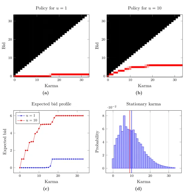
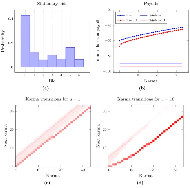
6 Society at Equilibrium 55 6.1 Default parameters . . . 55
6.2 Stationary Nash equilibrium computations . . . 57
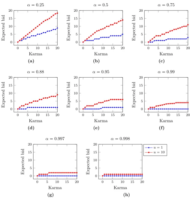
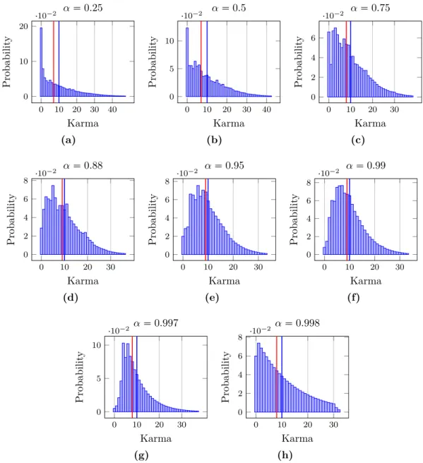
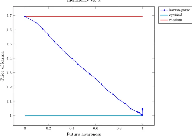
6.3 Effect of agents’ future awareness . . . 61
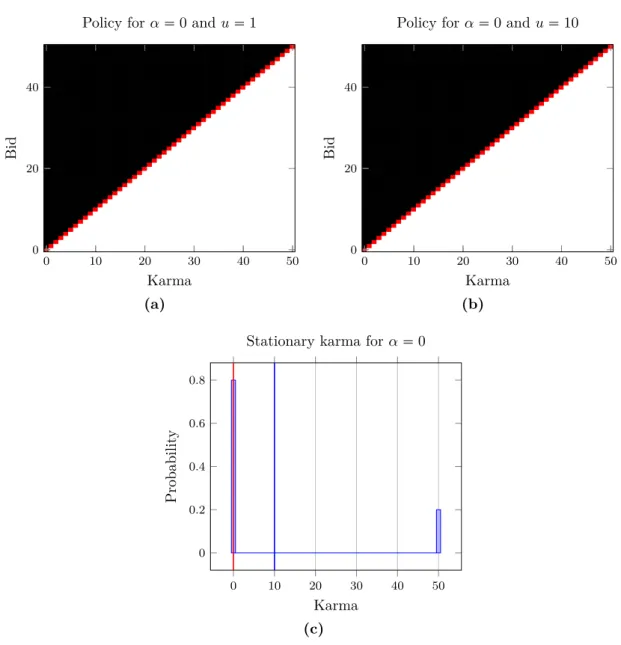
6.3.1 No future awareness . . . 61
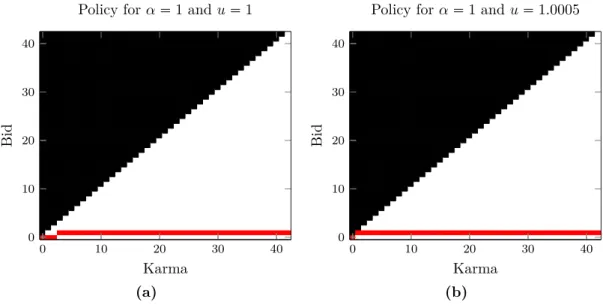
6.3.2 Infinite outlook . . . 63
6.3.3 Range of future awareness values . . . 65
6.4 Effect of the high to low urgency ratio . . . 71
6.5 Effect of a prolonged urgency stay . . . 73
6.6 Social welfare computations . . . 76
6.7 Effect of the average karma in the society . . . 78
7 Numerical Simulations 81 7.1 Social fairness . . . 81
7.1.1 Definition . . . 81
7.1.2 Benchmark fair resource allocation schemes . . . 82
7.2 Simulation parameters . . . 83
7.3 Simulation results . . . 84
8 Conclusions 87 9 Acknowledgements 89 A Discussion of the Assumptions of the Karma Game 91 B Derivation of the Population Dynamics 93 C Miscellaneous Proofs 95 C.1 Proof of Lemma 4 . . . 95
C.2 Support for the proof of Theorem 7 . . . 98
D Computational Heuristics 99 D.1 Discretization of the evolutionary dynamics . . . 99
D.2 Multi-valued best response . . . 99
D.3 Bounded karma values . . . 100
D.4 Convergence . . . 101
D.5 Uniqueness . . . 103
D.5.1 Uniqueness of the stationary population distribution for a policy . . . 103 iv
v
vi
Introduction
In this chapter, we introduce the problem at hand, and refer to the literature where appropriate.
Section 1.7 summarizes the main contributions of this work.
1.1 The resource allocation game
Consider a game where 2 agents compete over a finite resource. Each agent has a certain level of need for the resource, which we call the urgency of the agent and denote by u. If an agent gets allocated the resource, they incur zero cost, otherwise they incur a cost equal to their urgency. The agents have two actions available:yield (Y) oracquire(A). Figure 1.1 demonstrates a motivating example in intersection management, and Table 1.1 shows the cost matrix of this game. Entry pc1, c2qof the table denotes the cost to the respective agent. The resource cannot be allocated to both agents simultaneously, which is denoted by a cost ofU "u. This can be thought of as the agentscrashingin competition over the resource.
Figure 1.1: [1, Fig. 1] A motivating example of the resource allocation game is the problem of intersection management. Two cars compete over the right of way at an intersection. The passing agent incurs no cost, while the delayed agent incurs a cost that is equal to theirurgency. Who gets to pass?
1
2 1.2. Centralized allocation
Agent 2
Y A
Agent 1 Y pu1, u2q pu1,0q A p0, u2q pU, Uq Table 1.1: The resource allocation game
Highlighted are the twoNash equilibria of this game: (Y,A)and (A,Y). They areinadmissible; (Y,A)is beneficial to agent 2 but hurtful to agent 1, and vice versa for (A,Y). Which one will they play? Why would an agent compromise for the good of the other? This is a game where self-interested Nash equilibrium play fails to predict behaviour. At the heart of the problem lies the need for aresource allocation scheme which gives preference to an agent over another.
1.2 Centralized allocation
Suppose that agent 1 is more urgent than agent 2, i.e., u1 ¡ u2. This provides an avenue to break the deadlock: give the resource to agent 1 since they need it more. If the agents’ urgency representsthe value to society in allocating the resource to them, this is also the socially optimal action. For example, agent 1 can be a business owner on route to seal an important deal and agent 2 can be going on a leisure trip to the park. This is an instance ofcentralized allocation, where a central unit takes the most efficient decision on behalf of the agents. Much attention has been given to characterize the price of anarchy that the society has to pay as a consequence of self-interested behaviour, which cannot outperform centralized allocation in terms of efficiency [2].
However, centralized allocation is only an ideal. It does not scale well as the number of agents gets large, does not preserve privacy, and is prone to malicious attack. More fundamentally, it assumes that the central unitknows the urgency of all agents; an assumption that only holds true if the agents are all part of one (small) cooperative system. In practice, agents have tocommunicatetheir urgency in one way or another. What stops them then fromfooling the centralized unit in how badly they need the resource?
1.3 Auctions
One option is to give theownershipof the resource to the central unit, which thenauctionsits use out to the agents. The highest bidding agent gets the resource and incurs some cost in the form of a payment for its use. In our example, if the efficiency of centralized allocation is to be maintained, one would want to make sure that the more urgent agent 1 bids more than the less urgent agent 2. This is an instance of the problem oftruthful bidding in auction mechanism design, which the well-known Vickrey-Clark-Groove (VCG) mechanism guarantees [3].
Auction-based resource allocation schemes have been studied in the past. The well-known pro- portional allocation mechanism considers the allocation of an infinitely divisible resource among a finite number of competing agents [4, Chapter 21]. This departs from our setting since the re- source here is indivisible. Specifically in the field of intersection management, several auction-based schemes have been proposed, of which [5] is a representative example. There, anintersection man- agerruns a variant ofsecond price auctionsto schedule the right of way to vehicles at the front of the intersection, with results that suggest an improvement in trip times compared to traditional schemes such asfirst come first serve.
But even with truthful bidding, an auction-based approach to the resource allocation game at hand is problematic. Theownership of the resource by the auctioning unit is unwarranted; this unit is collecting payments from the agents but not contributing to society itself. Further, we must borrow an external resource, money (if monetary auctions are assumed), to settle the resource allocation.
This means that the problem is only shifted, since agents must compete over money elsewhere.
It also means that, as system designers, we do not have control over matters of fairness, since the agents’ budgets come from the outside, and are beyond our reach. So rich agents can starve poor agents out of the use of the resource. Fairness is indeed recognized as a challenge in the auction-based intersection management scheme of [5]. It is dealt with through the intervention of a benevolent system agent that makes anti-starvation adjustments to the auction mechanism. These adjustments are heuristic in nature, and go against the spirit ofcompletely decentralized control. In other applications such as networking and cloud computing, fair resource allocation has received some attention [6, 7, 8, 9]. In [6], for example, thefive axioms for fairness measures in resource allocationare defined. However, these works are concerned with aspacial rather than a temporal notion of fairness. Given a set of resources and a set of demands, how should the resources be split in a fair way? This deviates from the notion of fairness considered here which deals with the question of how to ensure that agents are not consistently favored over time.
1.4 The Karma game: A decentralized, efficient and fair re- source allocation scheme
In continuation to previous work [1], we propose a novel resource allocation scheme which we call thekarma game. The karma game is similar to traditional auction settings in that agents submit bids to acquire the resource. However, instead of bidding a monetary quantity, agentsbid karma, a quantity of which there exists a limited amount in the system that is preserved and circulated in the society, directly from agent to agent. Further, an agent cannot bid more karma than they currently own, which establishes a fundamental link between agents’ actions now and where they will be in the future. An agent can bid lots of karma now to guarantee a win, but they will consequently lose bidding power for the next time, when they perhaps really need it. This gives the karma game the following advantages for resource allocation.
1. No one owns the resource. Karma is exchanged among the agents directly. The winning agent pays karma to the losing agent. This leads to completely decentralized control and one has to only ensure that agents will abide by the karma game protocol. This can be ensured by a) designing the protocol in a way that makes it favorable for agents to abide by it, and b) through the use of decentralized accounting techniques, such as those implemented in blockchain technology [10]. The implementation of the protocol is not a focus of this work.
2. Incentive compatibilityis automatically achieved. It is not in an agent’s best interest to overbid to guarantee a win now as this will hurt their future. Any agent withsufficient future awareness will make sure tobid just the right amount now. Efficiency is to be expected.
3. Karma is self-contained. The agents do not need to borrow a resource from the outside to settle the problem, and there are no external differences in the agents’ budgets. Fairness is to be expected.
1.5 Repeated games
The problem of explaining the seemingly paradox cooperative behaviour that species exhibit, and that allows them to flourish, has received much attention in evolutionary biology (see, for example, [11] and references therein). In these works, the prototypical device for modeling outcomes of selfish versus cooperative behaviour is theprisoner’s dilemmagame. It is found that, while cooperation is never explained if agents were to play single instances of the game, cooperative strategies such as tit for tatandPavlovdo emerge as Nash equilibria when the game is infinitely repeated, provided that the agentscare enough about the future. The karma game is also an infinitely repeated game, and we will see comparable trends manifest in it. We note, however, that the resource allocation game at hand deviates from the prisoner’s dilemma. Here, one agent mustcollaborateand the other defect, and the concern is how to assign these roles, whereas in the prisoner’s dilemma, the concern is to incentivize collaboration by both agents.
4 1.6. Population games with dynamics
1.6 Population games with dynamics
The karma game setting inherits characteristics of the well-studied class ofpopulation games [12].
It is an infinitely repeated game between anonymous members of a society with a large number of agents. In the classical population game, each agent belongs to one of a number ofpopulations or types, where the size of each population is a static parameter. As it will turn out, the karma game can be similarly formulated, but requires that the populations be dynamic, i.e., that agents can transition into and out of the different populations.
Previous work has considered population games with payoff dynamics, where the typically static payoff map is replaced with a dynamical system that hashidden states, referred to as the payoff dynamics model [13]. This was inspired by the observation that evolutionary dynamics, which model how agents revise their strategies in population games, applied to the class ofstable games constitute a feedback interconnection of passive dynamical systems. This meant that the class of stable games can be generalized to games that have payoff dynamics with certain passivity properties [14]. Some proposed examples of payoff dynamic models which satisfy these properties included delay and smoothing of affine payoffs. An interesting application followed in [15], where a water distribution system was controlled using evolutionary dynamics. There, the dynamics of the physical water system were cleverly incorporated in the payoff dynamics model, and the stability of the feedback interconnection between the payoff dynamics model and the evolutionary dynamics implied the stability of the closed-loop water distribution system. Notably, afeedback lawfrom the states of the physical system, which are the hidden states of the payoff dynamics model, to its actuators was not explicitly stated.
These efforts do not capture the class of dynamics that arise in the karma game. Here, the agents themselves change their states, rather than the states being hidden in how they perceive their payoffs. The agents have different objectives, as well as different sets of admissible strategies, depending on the state they find themselves in. Therefore, states fit most naturally under the pre- existing notion of populations, with the exception that populations now need to be dynamic. With this dynamism, the strategies of the different populations get a new interpretation asfeedback laws from population to action. Inspired by the karma game, we introduce a new, general class of games which has not been studied before, which we calldynamic population games.
Population dynamics, which is a term that we will use here, arise in the field ofevolutionary game theory[16]. There, the dynamics are in terms of how populations of species grow or shrink according to their fitness over long time scales. This is completely different than the dynamics considered here, in which agents transition between populations at every instance of game-play. Interestingly, however, some works in the field ofevolutionary biology come close to the setting considered here, of which [17] is a representative example. This work studies kleptoparasitic behaviour in species, that is, whether species prefer to hunt for prey or steal it. There, animals take dynamic roles, such as whether they are searching for food or handling it, and the transitions between these roles depend on their actions, such as whether they hunt for food or wait for an opportunity to steal it.
These roles hence show resemblance to what we refer to here as dynamic populations. However, the dynamics that arise in such works tend to be specific to the problem at hand, and the resulting games are often treated as static at the rest points of the dynamics, which, in the case of [17], are straightforward enough to compute in closed form.
Finally, we note that the games with a dynamic population, as studied in [18], are different from the class of dynamic population games presented here. There, a single population of agents is considered, and the dynamics are in thepopulation size, i.e., agents are allowed to enter and exit the system. In contrast, the dynamic population games investigated here have multiple populations of agents, and they transition between the populations, but remain in the system.
1.7 Contributions
The following is a summarizing list of the most significant contributions of this work.
1. A mathematical formalization of the karma game as a tuple of game tensors, in Defi- nition 1. The game tensors compactly express the rules of the game, simplify analysis, and allow for flexible extension.
2. An attempt at classifying the karma game in the existing Game Theory literature in Chapter 2 Section 2.3, leading to the conclusion that while the karma game shows similarities to some existing classes of games, it stands in a class of its own.
3. The theoretical foundations for the new class of dynamic population games, in Chapter 3. This is considered the main contribution of this work. Among the main re- sults are Theorem 3, which establishes the existence of the newly introduced notion of thestationary Nash equilibrium, andTheorem 4, which establishes an equivalency between dynamic population games and classical population games.
4. A classification of the karma game as a dynamic population game, in Chapter 4.
Among the main results isTheorem 6, which establishes the fundamental notion ofkarma preservation, and is needed for the general results of dynamic population games to apply to the karma game. This classification leads to a mature characterization of agents’ rational behaviour in the karma game, and an algorithm to compute it.
5. A theoretical analysis of the social efficiency, in Chapter 5. Among the main results is Theorem 7, which gives a necessary and sufficient condition for any resource allocation scheme to achieve the optimal efficiency, and provides key intuition on the efficiency in the karma game.
6. An extensive numerical analysis in Chapters 6–7, which exposes the emerging trends of societal behaviour in the karma game, and highlights conditions where it achieves good efficiency and fairness. Some minor results and conjectures are presented.
6 1.7. Contributions
The Karma Game
In this chapter, we formally introduce the karma game, describing the game setting and rules in Section 2.1. Mathematical formalization succeeds in Section 2.2, which details the notational conventions followed. The main result of this chapter appears in Subsection 2.2.3 with a formal definition of the karma game as a tuple of game tensors (Definition 1). The game tensors compactly express the rules of the karma game, simplify analysis, and allow for flexible extension.
A classification of the karma game in the Game Theory literature follows in Section 2.3. We highlight that, while similarities exist to a number of game classes, the karma game stands in a class of its own.
2.1 The rules of the Karma game
Consider a society ofN t1, . . . , nauagents. Typical agents are denoted by i, j P N, with the typical viewpoint of an agentiasme and an agentj asmy opponent. Over their lifetimes, agents interact many times with each other. Letti P Z denote a discrete time index that increments each time agenti is involved in an interaction. We associate two quantities to agentiat timeti:
uiptiq:Urgency of agent i, kiptiq:Karma of agent i.
The urgency represents theneed of the agent, and the karma is a non-negative integer. At each interaction, two agents compete over one resource, i.e., they play the resource allocation game introduced in Chapter 1 Section 1.1. The resource allocation scheme proceeds as follows. Each agent i in the interaction submits a bid 0 ¤ biptiq ¤ kiptiq, and the resource is allocated to the agent with the highest bid. In the case of a tie, the resource is allocated on a fair coin toss. The winning agent, i.e., the one who gets allocated the resource, incurs zero cost but must pay karma to the losing agent, according to some payment rule. In turn, the losing agent incurs a cost equal to their urgencyuiptiq, but acquires karma from the winning agent.
2.1.1 Assumptions
We state the assumptions of the karma game here, and refer the reader to Appendix A for a discussion.
Assumption 1. Agents form a continuum of mass. The number of agents na is large. A single agent is small. Interactions are anonymous.
Assumption 2. The interaction timesticorrespond to rings of independent Poisson alarm clocks with identical rates for all agentsi PN. There is no synchronization between the agents’ clocks.
7
8 2.1. The rules of the Karma game
Interactions are viewed from the lens of a single agentiwho is interacting with the environment, rather than as interactions between two particular agentsiandj whose clocks ring together.
Assumption 3. Urgency is a discrete random variable with finite support, and takes on positive values. The time evolution of the urgency follows an exogenous Markov chain that is independent for each agent. The Markov chains are identical for all agents that belong to one of a finite number of urgency types. The Markov chain of each type has only one closed communicating class.
2.1.2 Payment rules
At every interaction, the winning agent must pay karma to the losing agent, according to apayment rule. Letpiptiqdenote the karma that an agentipaysin the interaction at timeti, such that their next karma iskipti 1q kiptiq piptiq, and consider an interaction between an agent iand an agentj at their respective time instancesti andtj. The payment rules must satisfy the following properties:
1. A strictly1 highest bidder pays karma:biptiq ¡bjptjq ñpiptiq ¡0¡pjptjq.
2. Karma is preserved:piptiq pjptjq. The amount of karma that agentipays is equal to the amount of karma that agentj gets paid, and vice versa. This means that thetotal karma is preserved in the interaction:kipti 1q kjptj 1q kiptiq kjptjq.
3. An agent never pays more karma than they bid:piptiq ¤biptiq. It follows that the karma of an agent can never become negative, sincebiptiq ¤kiptiq. It also follows thatpiptiq ¤bjptjq.
1There is flexibility in the case of a tie biptiq bjptjq, as long as the other payment rules are adhered by.
The following are threeexamplesof payment rules.
1. Pay as bid:biptiq ¡bjptjq ñpiptiq biptiq pjptjq. In the case of a tiebiptiq bjptjq, the winning agent (as decided on a fair coin toss) pays their full bid to the losing agent.
2. Pay as other bid: biptiq ¡bjptjq ñpiptiq bjptjq pjptjq. In the case of a tie bi bj, the winning agent (as decided on a fair coin toss) pays their full bid to the losing agent, which is equal to that agent’s bid.
3. Pay difference:piptiq biptiq bjptjq pjptjq. Note thatpiptiq ¡0 holds automatically whenbiptiq ¡bjptjq. Note also that in the case of a tiebi bj, the winning agent is decided on a fair coin toss as usual but zero karma is exchanged.
The examples highlight that there is a degree of freedom in the design of the karma game system.
The analysis results herein apply to any payment rule satisfying the properties above, but we only considerpay as bid in the numerical investigations of Chapters 6–7. Pay as bid can be viewed as an adaptation of thefirst price auction.
2.2 Formalization
With the karma game rules introduced, we now turn to mathematical formalization.
2.2.1 Notational conventions
The following notational conventions are used for convenience whenever they do not lead to a loss of context. We note that they are not always followed, and we switch to more explicit notation at times without forewarning. We apologize to the reader for the confusion that may arise.
I am agent i, and my opponent is agentj.
The viewpoint of an agent i (me) against a world with agents j (my opponent) is taken. The superscript ‘i’ is dropped, and all quantities are related to me by default. On the other hand, the superscript ‘j’ persists and denotes quantities related to my opponentj. For example,uptqdenotes my urgency, whileujptjqdenotesmy opponent’s urgency.
Only the last, current and the next times are relevant.
In what follows, all time evolving quantities follow a first order Markov chain, and the only relevant time indices aret (current time),t1 (last time) andt 1 (next time). The dependence on time is dropped in notation, last time quantities are denoted by the superscript ‘’, and next time quantities by ‘ ’. For example, the current urgencyuptqis simply denoted byu, the last urgency upt1qbyu, and the next urgencyupt 1qbyu .
Einstein notation and tensor operations.
Einstein notationis adapted to compactly express the abundance of sums resulting from the many expectation operations to follow. Operations occur ontensorswith sub- and/or superscript quan- tities. A convention is followed whereinput quantitiesappear in subscript, and output quantities in superscript. We define two types of tensors:
1. Functional tensors represent functions of input variables and have subsript quantities only. For example, the interaction costcto an agent is a function of their urgencyuand the outcome of the interactiono, written innormal form ascpu, oq. We denote it intensor form bycu,o. One can interpret the tensorcu,o as apre-computed table of the functioncpu, oqfor all input value pairspu, oq.
2. Probability tensors represent marginal probabilities if they have superscript quantities only and conditional probabilities if they have both sub- and superscript quantities. Let pO1, O2, . . . , I1, I2, . . .q be random variables with realizations o1, o2, . . . , i1, i2, . . ., respec- tively. Then, we define a probability tensorpby
poi11,i,o22,...,...:P O1o1, O2o2, |I1i1, I2i2, . . . ,
i.e., the tensor p holds the conditional probability table of the superscript (output) quan- tities conditioned on the subscript (input) quantities. If there are no subscript quantities, then tensorpsimply holds the marginal probability table of the superscript quantities. For example, the outcome of an interactionois a random variable whose probability depends on the bidsbandbj, and tensorγb,bo j holds this conditional probability table. Another example is tensorνbj, which holds the probability distribution of opponents’ bids.
In general, probability tensors are denoted simply by p and the reader is to rely on their sub- and superscript quantities to infer what probability distribution they refer to. Some probability tensors are given specific symbols to highlight their role, such as the two examples γob,bj and νbj above. In all cases,a tensor with superscript quantities is a probability tensor, in the context of this document.
10 2.2. Formalization
A sub-class of probability tensors are transition tensors, which denotetransition proba- bilities of Markov chains. An example is φuu,µ, which holds the transition probability of an agents urgencyutou , conditional on the urgency typeµ.
The following are two examples that demonstrate the use of tensor operations.
Example 2.2.1. ζpu, b, bjq is the expected interaction cost to an agent as a function of their urgency, bid, and their opponent’s bid. Innormal form, it is given by
ζpu, b, bjq E
o
cpu, oq |b, bj ¸
o
γpo|b, bjqcpu, oq,
and intensor form by
ζu,b,bj γb,bo j cu,o.
Note how a quantity appearing both as a sub- and superscript in the tensor operation,o in this case, is marginalized and does not appear in the output tensor.
Example 2.2.2. Suppose that the policy of the opponentsπbujj,kj, as well as the joint probability distribution over their urgency and karmaduj,kj, are given. Then the probability of encountering a bidbj in is given innormal form by
νpbjq ¸
uj,kj
dpuj, kjqπpbj|uj, kjq,
which is an application of themarginalization rule. Intensor form, it is given by νbj duj,kj πubjj,kj.
Note again how quantities appearing both as sub- and superscripts in the tensor operation are marginalized.
The examples demonstrate how what we have referred to as thetensor form compacts the expec- tation operations in comparison to what we have referred to as thenormal form. We will however revert to the normal form at times when it is insightful to do so. The reader is expected to adapt to either form based on the context.
2.2.2 Definitions
The following is a list of the definitions of the elementary quantities in the karma game. More definitions will appear in the text at their appropriate context.
naPZ is thenumber of agentsin the society, assumed to be large.
ktot P Z is the total amount of karma in the society. ¯k P Q is the average amount of karma, which is normalized by the large number of agents, i.e.,¯k kntota . We usek¯to characterize the amount of karma in the society, which is adesign parameter.
µ P M 1, . . . , nµ
( is an agent’s urgency type, which characterizes their urgency Markov chain. There arenµ urgency types.
αPA α1, . . . , αnααlP r0,1q @l1, . . . , nα
(is an agent’sfuture awareness type. There arenα future awareness types.
The concatenationτ pµ, αq PT MA is simply an agent’s type. The number of types is nτnµnα.
gP∆nτ is thetype distribution, written in tensor form asgτorgµ,α. This is asetting parameter.
ψ:T Ñ∆nτ is thetype Markov chain, written in tensor form asψττ orψµ ,αµ,α . This encodes that an agent’s type isstatic, and is given by theidentity transition tensor
ψττ
#1 :τ τ, 0 : otherwise.
uPU
$&
%u1, . . . , unu
ulPR @l1, . . . , nu
ul¡0 @l1, . . . , nu
ul ul 1 @l1, . . . , nu1 ,.
-is an agent’surgency, which takes one ofnupositive real values in an ordered set.
k P K tkPZ |k¤ktotu is an agent’s karma, a non-negative integer counter that cannot exceed the total amount of karma in the society. There arenk ktot 1 possible values of karma.
See Remark 2.2.1.
The concatenationx pu, kq PX UKis an agent’sstate. The number of states isnxnunk. The concatenationρ pτ, xq PP T X is an agent’s population. The number of populations isnρnτnx.
φ : MU Ñ ∆nu is the urgency Markov chain, written in tensor form as φuu,µ. Urgency transition probabilities are conditional on the agent’s urgency typeµ. This is asetting parameter. bPBpkq tbPZ |b¤ku Kis an agent’sbid, which cannot exceed their karma.
oPO t0,1uis theinteraction outcome to an agent. o0 denotes that the agent wins the resource and incurs zero cost, and o 1 denotes that the agent loses the resource and incurs a cost. The number of possible interaction outcomes isno2.
γ:KK Ñ∆no is theprobability of the interaction outcome to an agent given their and their opponent’s bid, written in tensor form asγb,bo j. From the rules of the game, it is given by
γob,bj
$' '' '&
'' ''
%
1 :b¡bj, o0, 1 :b bj, o1, 0.5 :bbj, 0 : otherwise.
(2.1)
c : U O Ñ R is the interaction cost incurred by an agent given their urgency and the interaction outcome, written in tensor form ascu,o. The cost is non-negative. From the rules of the game, it is given by
cu,ou o. (2.2)
p P Ppb, bjq pPZ bj ¤p¤b(
pKX Kq is the karma payment by an agent in an interaction. A negative value implies that the agentgets paidkarma. An agent can pay at maximum their bid and get paid at maximum their opponent’s bid.
δ: KKO Ñ∆2nk1 is theprobability of the karma payment by an agent given their bid, their opponent’s bid, and the interaction outcome, written in tensor form asδpb,bj,o (see Re- mark 2.2.2). This encodes thepayment rulefollowed. Forpay as bid, it is given by
δpb,bj,o
$' '&
''
%
1 :pb, o0, 1 :p bj, o1, 0 : otherwise.
12 2.2. Formalization
η:K pKX Kq Ñ∆nk is theprobability of the next karmaof an agent given their current karma and the karma they pay, written in tensor form asηk,pk (see also Remark 2.2.2). From the rules of the game, it is given by
ηk,pk
#1 :k kp,
0 : otherwise. (2.3)
Remark 2.2.1. The number of possible karma values nk is large since ktot is large. We use it here as a theoretical upper bound which implies that the karma state-space is finite. Appendix D Section D.3 demonstrates how a small practical upper bound can be used for computation.
Remark 2.2.2. p is deterministic in pb, bj, oq, and k in pk, pq, but we choose to express these dependencies as probability distributions since they are used in the upcoming derivation of the karma Markov chain (2.4).
2.2.3 The Karma game tensors
We are now ready to present a formal definition of the karma game.
Definition 1(Karma game).
A karma game is a tuple ofgame tensors
k,¯ gτ, ψττ , φuu,µ, κkk,b,bj, ζu,b,bj .
¯kis the average amount of karma in the society, a zero-dimensional tensor (scalar).
gτ is the type distribution, a probability tensor.
ψττ is the type Markov chain, an identity transition tensor which signifies that types are static.
φuu,µis the urgency Markov chain, a transition tensor. It is conditional on the agent’s urgency type.
κkk,b,bj is the karma Markov chain, a transition tensor. It is conditional on the agent’s bid and their opponent’s bid.
ζu,b,bj is the expected interaction cost, a functional tensor of the agent’s, urgency, bid, and their opponent’s bid.
The karma game tensors are a compact mathematical representation of the rules of the game. They encode all the properties of the game which do not depend on the agents’ behaviour. We have seen
¯k, gτ, ψττ and φuu,µ in the elementary definitions of Subsection 2.2.2. The last two tensors are composed from those definitions as
κkk,b,bj γb,bo jδpb,bj,oηk,pk , (2.4)
ζu,b,bj γb,bo jcu,o. (2.5)
The game tensors are used extensively in Chapter 4 to simplify the analysis. They also allow for flexible extensionsto the karma game, as the following example demonstrates.
Example 2.2.3 (Karma game extension). Consider the following modification to the rules of the karma game. When agents tie on their bids, the resource is allocated to the agent with more karma, since they are likely to have suffered more in the recent past. It is straightforward to incorporate this modification with the karma game tensors. We add dependencies on the agent’s and their opponent’s karma to theprobability of the interaction outcome(2.1), which now becomes γk,b,ko j,bj. The new dependencies then naturally appear in thekarma Markov chain, which becomes κkk,b,kj,bj, and theexpected interaction cost, which becomesζu,k,b,kj,bj. No further work is required.
We note that Example 2.2.3 is presented merely to show off the flexibility of the karma game tensors formalization. Although the example modification is sensible, it requires a degree of centralized control to enforce. Also, the increased dimensionality of the game tensors bears a computational burden, both tostore the tensors and toprocess operations on them.
14 2.3. Classification of the Karma game
2.3 Classification of the Karma game
To develop intuition on the newly introduced karma game, we attempt to draw relations to some existing and well-studied classes of games in the literature. This is particularly insightful for shed- ding light onhow rational agents ought to behave in the karma game. Table 2.1 summarizes the main comparison points to the game classes considered.
Game class Similarities Differences
Bayesian games Incomplete information Finite number of agents
Distribution of opponents is given Dynamic games Agents have dynamic states Finite number of agents
Dynamics depend on actions Finite number of stages Agents consider future when strategizing Complete information Stochastic games Markovian dynamics Finite number of agents
Dynamics depend on actions Dynamics are on common game state Discounted infinite horizon payoffs Agents observe game state
Evolutionary games Population dynamics are considered Dynamics are related to fitness Population games Large number of agents Distribution of opponents is given
Incomplete information No dynamics
Table 2.1: Karma game classification
2.3.1 Relation to Bayesian games
Bayesian games are games with incomplete information, where agents take one of a number of types. Agents of different types have differing goals and are expected to behave heterogeneously.
An agent only knows their own type but not that of their opponent, i.e., the type is a private value. The standard assumption in Bayesian games is that thedistribution of opponents’ types is known, and hence an agent can devise optimal strategies based on theexpected behavior of their opponents, leading to the so-calledBayesian Nash equilibrium condition [19].
The karma game is also a game with incomplete information; agents are anonymous and in an interaction, an agent does not know their opponent. We have defined the agent typeτ pµ, αq and specified the type distributiongτ, in the spirit of the classical Bayesian game. But in addition to their type, an agent will behave differently based on theirstate x pu, kq. A higher urgency agent will be inclined to bid more than a lower urgency one, and an agent with lower karma will be inclined to bid less than one with higher karma, who has more bidding power. So, if an agent is to reason about the expected behaviour of their opponents, they will require a probability distribution over their types and their states. Only the former is given, and the latter requires new analysis tools. This is precisely where the karma game deviates from the classical Bayesian game.
To give a preview, we will need to to look for stationary distributions of the state x pu, kq Markov chain. If we suppose that agents are particles that independently traverse this chain, which is warranted by Assumptions 1–3, then, after some time, the distribution of the states of these particles will coincide with a stationary distribution of the Markov chain (under some technical assumptions). For the exogenous urgency Markov chainφuu,µ, the stationary distribution is straightforward to compute. But the karma Markov chain κkk,b,bj is a function of the agents’
behaviour, which further complicates matters.
Before concluding this discussion, we note that in the karma game, an agent need not care about the distribution of the opponents’ types and states, at least not directly. It suffices to have an estimate of thedistribution of the opponents’ bids, which we denote byνbj. For example, they can learn it directly from their history of interactions. This follows by investigation of the karma game
tensors, where dependency on the opponentsj only appears in the form of their bidsbj. We will see next howνbj is all an agent needs to compute abest response.
Remark 2.3.1. If, as in Example 2.2.3, a dependency on the opponent’s karmakj is added, then an agent needs to learn a joint distribution over the opponents’ karma and bids, etc..
2.3.2 Relation to dynamic and stochastic games
If the point of view of a single agent interacting with the uncertain environment is taken, their statex pu, kqevolves as astochastic discrete-time dynamical system, which can be abstracted as
xpt 1q
upt 1q kpt 1q
wµpuptqq wkpkptq, bptq, bjptqq
, (2.6)
wherewµpuqandwkpk, b, bjqdenotestochastic disturbances that can be derived from the Markov chainsφuu,µandκkk,b,bj, respectively.
Similarly, one can define astochastic stage cost function to the agent as cptq c
uptq, wopbptq, bjptqq , (2.7)
where wopb, bjqdenotes a stochastic disturbance on the interaction outcome and can be derived fromγob,bj.
In Equations (2.6)–(2.7), both the agent’s bidband their opponent’s bidbj enter asinputsto the dynamical system. But, to the agent,bjis itself stochastic, and can be incorporated in the stochastic disturbance models if knowledge of its distributionνbj is supposed. Withbj eliminated, the agent’s bidb becomes the only input to Equations (2.6)–(2.7), which now constitute the building blocks of adynamic programming problem[20, Chapter 1]. Optimal bidding strategies will correspond to solutions of that problem. This exposes a relation to dynamic games, where Nash equilibria are computed usingbackward induction, the game-theoretic term for dynamic programming.
However, backward induction as applied to the classical dynamic game requires a finite number of agents, a finite number ofgame stages, deterministic dynamics, and complete information about the opponents. The karma game does not satisfy these requirements, and cannot be directly classified as a classical dynamic game.
Stochastic games[21], which are also known asMarkov games, can be viewed as a generalization of classical dynamic games that accounts for stochastic dynamics, which we have here. A formulation of these games that considersdiscounted infinite horizon payoffsinstead of a finite number of game stages exists, which aligns nicely with the infinitely repeated karma game. But the challenges of a finite number of agents, and complete information, persist in classifying the karma game as a stochastic game. There, the stochastic dynamics are on a commonly evolvinggame state, which all agents observe at every game stage. This stands in contrast to the dynamically evolving urgency and karma in the karma game, which are private to each agent. The resemblance is still apparent though, in the nature of the dynamics, and in how agentsconsider their future when strategizing. We will see thatbest responsesin the karma game correspond to solutions of dynamic programming problems, much like in dynamic and stochastic games.
2.3.3 Relation to population games
The karma game setting was largely inspired by the class ofpopulation games, which, like in the karma game, considers game-theoretic interactions in a society of a large number of anonymous agents [12]. Among others, Assumption 1 is directly adapted from the assumptions of population games, and exposes the resemblance.
In the classical population game, agents belong to one of a finite number ofpopulations, and the relative size of each population is a given parameter. Agents of the same population are identical in
16 2.3. Classification of the Karma game
their motifs and the strategies available to them, and hence behave the same. It is no coincidence that in the karma game we use the termpopulation to refer to the concatenation of agents’ type and stateρ pτ, xq, which we view as the karma game equivalent. The typeand the state is what makes agentsidenticalin the karma game; agents of the same type but different states will behave differently, and vice versa. Byidentical behaviour here we mean that in one instance of game-play, agents will play the same strategy, or randomize over their strategies using the same probability distribution.
However, in the classical population game, populations arestatic and correspond more closely to the notion of agenttypes as introduced in the context of Bayesian games (see Subsection 2.3.1).
Therefore, the same challenge in classifying the karma game as a Bayesian game holds here. In particular, the dynamism in the agents’ state, and thereby their population, deviates from the classical setting.
It looks as though the karma game stands alone in respect to the existing classes of games, and new tools are required to analyze it. Inspired by the karma game, we introduce the new general class of dynamic population games, which can be viewed as a generalization of classical population games that allows certain classes of dynamics in the populations. The theory of dynamic population games is developed in the upcoming Chapter 3. Following, Chapter 4 demonstrates how the karma game falls under this new class, and, among others, uses the new framework to reason about agents’
rational behaviour.
Dynamic Population Games
In Chapter 2 Section 2.3, we drew relations between the karma game and some existing classes of games, and found that it stands in a class of its own. In this chapter, we take anabstraction step and depart completely from the karma game setting to introduce a newgeneral class of games. To this regard, this chapter is to be treated as astand-alone entity which has its own formalization and notation. We will return to the karma game setting in the next Chapter 4, where the general results of this chapter will be applied to mature our understanding of the karma game.
This chapter is considered the main contribution of this work, as it lays down the theoretical foundation for the analysis of the karma game, using a general framework that is non-restrictive to only the karma game. Among the results, we highlight two that are of most significance. The first isTheorem 3, which proves the existence of the so calledstationary Nash equilibriumin dynamic population games, and can be viewed as an extension of the well-known Nash’s theorem to this new class of games. The second isTheorem 4, which proves that dynamic population games can be cast as classical population games via anaugmentation, thereby establishing a fundamental link between the two classes of games.
The notation in this chapter is largely inspired by that of the classical population games as defined in [12], in an attempt to make the connection between the two classes of games apparent. It is particularly important to note that we do not follow Einstein notation in this chapter. So sub- and superscript quantities here are merely a matter of notational convenience, and do not hold the interpretation ofinputandoutput quantities assumed in large proportions of this text. In general, subscript quantities here take the familiar role of denoting elements of a vector.
3.1 Setting
Populations
Consider a societyN t1, . . . , nauof anonymous agents, withnalarge such that agents approxi- mately form acontinuum of mass m1. At any point in time, each agent belongs to apopulation ρPP 1, . . . , nρ
(, withnρ¥1.
Strategies and policy
Agents of the same population ρ are identical; they have the same motifs and the same set of strategies Sρ t1, . . . , nρsu, nρs ¥ 1, to choose from, and behave the same. Typical choices of strategies are denoted byior jPSρ. The total number of strategies isn °
ρPP
nρs.
Agents are allowed to randomize their strategy choice. Let πρ P Πρ ∆nρs denote the mixed strategy of agents in populationρ; a probability distribution from which they draw their strategy
17
18 3.2. Population dynamics
choice at every interaction. Elementπiρis the probability of playing strategyiPSρ. Ifπρeifor some strategyiPSρ, whereei is the elementary unit vector ini, we say thatπρ is apure strategy.
The concatenation of the mixed strategiesπ pπ1, . . . , πnρq PΠ ±
ρPP
Πρ is thepolicy.
Population distribution
Further, let d P D ∆nρ be the population distribution, where element dρ is the proportion of agents in the society belonging to populationρ P P. This distribution is allowed to be time- varying; agents belonging to one population is susceptible to transition to another, for instance, due to an exogenous process or as a result of game-play itself. We restrict our attention to Markovian population dynamics that aremass preserving, i.e., agents can transition from one population to another, but cannot leave the society, or, if they do, they are immediately replaced with new agents taking their place.
Social state
We refer to the pairpπ, dq PΠDas thesocial state, since they jointly describe the distribution of agents in the society and how they behave
Remark 3.1.1. In the population games literature, what we refer to here as the mixed strategy πρ and the policy π is popularly referred to as the population state xρ and the social state x, respectively [12, pp. 22–23]. This is because in the classical population game,πiρ(or respectivelyxρi) has an alternative interpretation as theproportion of agentsin populationρplaying pure strategy i. However, ifdρ, the mass of agents in populationρ, is time-varying, so can be the proportion of agents playing a certain strategy. Therefore, in the dynamic population game we insist on defining πρ as the mixed strategy of agents in populationρ, andπas the policy, and note that it does not vary in time unless agents revisetheir strategies. It is only when πis coupled withdthat one can fully describe agents’ behavior in society, and therefore we reserve the term social stateto the pair pπ, dqhere.
Remark 3.1.2. An agent transitioning from population ρ to ρ will play mixed strategy πρ in their next interaction, i.e., will imitate other agents in the destination population. This is reasonable since agents in that population are themselves rational. Therefore, the policyπbears the interpretation of afeedback law that tells an agent finding themselves in populationρto play πρ. Payoffs
The payoff to an agent from population ρ P P playing strategy i P Sρ is a continuous map Fiρ : ΠD Ñ R. The payoff vector of population ρ is Fρ : ΠD Ñ Rn
ρ
s, whose ith element is Fiρpπ, dq. F : ΠD Ñ Rn is the concatenation of the payoff vectors of the populations, i.e., Fpπ, dq F1pπ, dq, . . . , Fnρpπ, dq
, and is simply referred to as thepayoff vector.
Remark 3.1.3. Since in general an agent’s action affects what population they will transition to, it is sensible for agents to consider future payoffswhen strategizing. For now, we only require that the payoff vector Fpπ, dq be continuous. Section 3.6 demonstrates how Fpπ, dq can be defined to describe infinite horizon payoffs.
3.2 Population dynamics
Suppose that after every interaction, an agent of population ρ P P playing strategy i P Sρ is susceptible to transition to population ρ P P. We write tρ,i : ΠDÑ ∆nρ as the population transition vectorfor an agent of populationρplaying strategyi, where elementtρ,iρ is the probability of transitioning toρ . We require thattρ,ipπ, dqbe acontinuousmap, and note that sincetρ,ipπ, dq P
∆nρ @pπ, dq PΠD, the agent can transition to another population, but must remain in the society.
![Figure 1.1: [1, Fig. 1] A motivating example of the resource allocation game is the problem of intersection management](https://thumb-eu.123doks.com/thumbv2/1library_info/5353125.1682976/10.892.289.608.724.922/figure-motivating-example-resource-allocation-problem-intersection-management.webp)