INAUGURAL-DISSERTATION Zur
Erlangung der Doktorwürde Der
Naturwissenschaftlich-Mathematischen Gesamtfakultät Der Ruprecht-Karls-Universität
Heidelberg
Vorgelegt von Diplom-Mathematiker
John Wallis
Aus Aurora, Colorado
Tag der Mündlichen Prüfung:
11. Juli 2003
DEVELOPMENT OF A SPECTRALLY-RESOLVED
FLUORESCENCE 3D FOR LIFETIME IMAGING MICROSCROPY
PRECISION MEASUREMENTS IN THE NANOMETER RANGE
Gutachter: Prof. Dr. Jürgen Wolfrum
Prof. Dr. Joachim Pius Spatz
To my wife
ACKNOWLEDGMENTS
I would like to thank my wife for her endless moral support during this work. I would also like to thank my parents, my wife’s parents, and my sons, Charles and Philip. I would also like to thank all the people at the chemical and numerical sections of the University of Heidelberg for their support.
SUMMARY
This work developed a program to monitor and collect florescence photons from single molecules in three-dimensional domains with high precision and developed tools for viewing such data. The resulting scanned images reveals better understanding of the interplay between the molecules. These images also help the researcher find areas of interest and he can quickly measure in more detail these areas. This program was written with Microsoft's Visual C that interfaced with a Queensgate NPS3330 nanopositioning table and an SPC-630 time correlated single-photon detection card. Micrometer volumes can be scanned using confocal microscopy techniques during which single molecules tagged with fluorescent dyes are excited by a pulsed laser. In a few nanoseconds the dyes will fluoresce. Several (100-1000) photons will move in the direction of one or more avalanche diode detectors (APD) that send signals to the photon detection card. The SPC card receives and orders incoming photons and sums them forming a decay (lifetime profile) curve. The SPC-630 card has a configurable memory capable of storing many decay curves of short durations, usually in microseconds. Blocks of these curves are periodically saved to disk for post-analysis. In the post-analysis, the program enables the user to choose which channels he wishes to use for lifetime estimations.
Minimum/maximum boundary values can be given for a given variable for filtering permanent information. The user can also use previous scans to zoom in on certain domain areas. Information pertaining to selected individual pixels can be also collected and exported to other programs, such as Excel. This work developed a method for the 3D imaging of cells using spectrally – resolved fluorescence lifetime imaging microscopy (SFLIM)
TABLE OF CONTENTS
ACKNOWLEDGMENTS ...III SUMMARY...IV LIST OF TABLES ...VI LIST OF FIGURES ... VII
1. INTRODUCTION AND MOTIVATION ... 1
2. DESCRIPTION ... 11
3. MATERIALS AND METHODS... 13
3.1. QUEENSGATE NPS3330 ... 14
3.2. SPC 630 ... 17
3.3. THE PROGRAM ... 22
3.3.1. The Scanning... 22
3.3.2. Postprocessing... 27
3.3.3. Miscellaneous Dialogs ... 31
3.3.3. The Visualization ... 33
4. EXAMPLES... 34
4.1. A DEAD CELL... 34
4.2. BREAST CANCER... 36
5. DISCUSSION AND OUTLOOK ... 37
APPENDICES ... 40
A. INDEX OF ABBREVIATIONS... 40
B. THE SCANNING ROUTINES ... 42
C. THE SCANNED FILE FORMAT ... 48
D. PROGRAM FILES ... 49
Primary files ... 49
Secondary files ... 50
BIBLIOGRAPHY ... 51
LIST OF TABLES
Table 1: The Queensgate table used has been tested and the following results are
available. ... 15 Table 2: SPC memory allocation. ... 22
LIST OF FIGURES
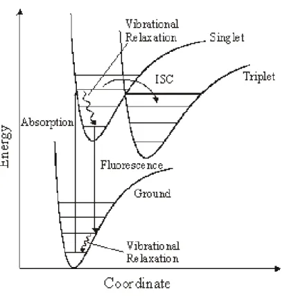
Figure 1: Potential energy curves and fluorescence cycle of a single-molecule. ISC
depicts intersystem crossing to the triplet state... 3
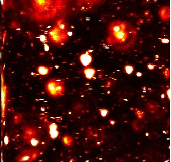
Figure 2: Test scan DiDDPPC of 30x30 µm area made by Ken Weston with no pinhole. Rings are caused by diffraction the light at the lens borders. ... 6
Figure 3: Airy Discs. The middle image is a blowup of an area of Figure 2. ... 6
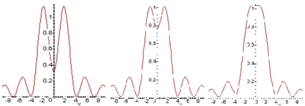
Figure 4: Figure Rayleigh Criterion: left to right: resolved, Rayleigh Criterion and unresolved. ... 7
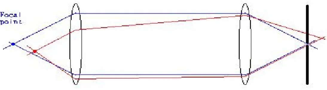
Figure 5: Confocal microscopy. Only light at the focal point is allowed through, thus eliminating blurs caused by out of focus light. ... 8
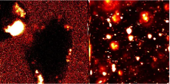
Figure 6: Left: 25*25 micron scan of a cell (black). The lighted spots are from CY5. Right: 30*30 microns scan by Ken Weston. ... 9
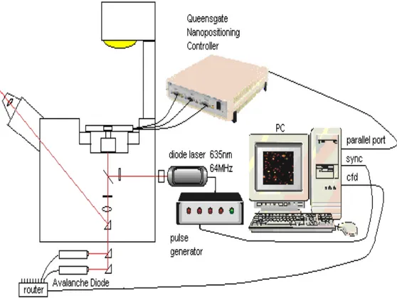
Figure 7: A typical scanning setup configuration. ... 12
Figure 8: A scan of a part of a 100-µm-scale slide. ... 15
Figure 9: Left to right: Scans using the sine waveform used for the x-direction, corrected position and fill-in. The y-axis (top to bottom) lines have a zigzag quality due to small delays in y stepping. Although the image can be corrected information of the individual pixels is not uniform. ... 16
Figure 10: Same 10*10 micron scan using sawtooth waveform... 16
Figure 11: The Queensgate nano positioning device NPS3330 XYZ... 17
Figure 12: SPC630 ... 18
Figure 13: The CFD adds a part of the inverted signal to the original signal to form a consistent temporal location of the detected photon pulse... 19
Figure 14: General principle of the TCSPC measurement using the SPC modules ... 20
Figure 15: The summation process of the SPC card to form a decay curve. ... 21
Figure 16: Queensgate waveforms used for the x-axis. From left to right: ramp and square. Scans using the rampwave option resulted in the clearest images being blurred only on one side due to measurements continuing during the resweep phase. Scans using the sawtooth wave possessed sub pixel blurring due to the y positioning delays at the edges... 23
Figure 17: flowchart of scanning procedure ... 25
Figure 18: SPC preview and adjustment dialog. ... 26
Figure 19: The main scanning dialog... 27
Figure 20: Postprocessing Dialogs: a.) At the top the d_post general viewing settings, b) at the center is a histogram/filter dialog, c) to the center/right is the decay view: the left mouse selects the actual decay shown. ... 29
Figure 21: snapshots: give information about individual or a group of photons, such as detector counts, lifetimes, fractional intensity and total intensity... 30
Figure 22: Snapshot: here the fractional intensities (y-axis) are plotted against the lifetime values (x-axis). Fractional intensities can help a researcher determine if one or several objects are present and their distance from each other. ... 31
Figure 23: A scan of an old cell without a pinhole. The scan resulted with cylindrical objects... 34
Figures 24: Dead cells. From left to right: 80x80 microns, 40x40 microns, 20x20 microns, and 10x10x10 microns at 3 pixels/micron. Laser intensity was set at 20 µwatts and a 50-µm pinhole was used. ... 35
Figure 25: Scans from Thomas Heinlein: Small area, approximately 15x15x5 microns at 10 pixels/micron, laser intensity set to 20 µwatts. Breast cancer cells marked with antibodies attached to the membrane. This antibody is detected by a secondary antibody marked with a Bodipy 630/650 (IgG). ... 36
Figure 26: The measurement volume... 37
1. INTRODUCTION AND MOTIVATION
The observation, manipulation, and controlling of matter at molecular and atomic scales has been a wish of scientists for many ages. Today many detection and observation techniques exist such as: scanning tunneling microscopy, and atomic force microscopy.
Optical methods have been developed to scan chemical species and their environmental interactions without contact from tips. Advancements in spectroscopy enable detection, identification and recording of dynamical processes of diffusing or immobilized molecules. Hirschfeld, in 1976, proved it is possible to detect certain molecules on a single antibody molecule labeled with 80-100 fluorescein molecules. (Hischfeld 1976) Room temperature detection of single immobilized fluorophores using near- and far-field (Betzig and Chichester 1993; Trautman, Macklin et al. 1994; Xie and Dunn 1994;
Macklin, Trautman et al. 1996) scanning techniques motivated scientists around the world. It is still in debate whether single molecule detection or ensemble measurements over time deliver new knowledge regarding molecular behavior.(Xie 1996) A fundamental postulate of statistical mechanics, the ergodic hypothesis, states that the time-average of a physical quantity along the trajectory of a member of the ensemble is equivalent to the average of that quantity at a given time over the ensemble. For the
ergodic hypothesis to be even approximately applicable the ensemble must consist of entirely equivalent members, i.e. it must be homogeneous. However, many chemical and biological systems are inhomogeneous. The inhomogeneity can be truly static, i.e. it arises from definable chemical differences. But, on the other hand, it was found that intermolecular variations persist even when there are no chemical differences. The key is the time scale over which the averaging is performed. Ensemble measurements provide average properties. Single molecule spectroscopy (SMS) and single molecule detection (SMD) using laser induced fluorescence, on the other hand, present information (distribution and time trajectories) on individual molecules and may discover properties that otherwise would remain hidden. Among the hidden properties are such quantities such as fluorescence intensity fluctuations due to spectral diffusion (Ambrose and Moerner 1991; Ha, Enderle et al. 1997; Lu and Xie 1997; Weston and Buratto 1998;
Weston, Carson et al. 1998; Ying and Xie 1998; Yip, Hu et al. 1998; Köhn, Hofkens et al. 2000), fluorescence lifetime(), triplet (Veerman, Garcia-Parajo et al. 1999; English, Furube et al. 2000; Weston and Goldner 2001) and rotational jumps(Ha, Enderle et al.
1996; Ruiter, Veerman et al. 1997; Bartko and Dickson 1999), as well as photon anti bunching.(Orrit and Bernard 1990; Ambrose and Moerner 1991; Basché, Kummel et al.
1995; Lounis and Moerner 2000; Michler, Imamoglu et al. 2000) These fluctuations are often observed as on/off intensity jumps. This “blinking” is accepted as an obvious criterion for a single-chromophore system. Laser-induced fluorescence (LIF) is now widely used because of its high signal to noise ratios. In the condensed phase fluorescence emission usually occurs in a four-step cycle (figure1.2): (a) electronic transition from the ground-electronic state to an excited-electronic state; (b) internal relaxation in the excited-electronic state; (c) radiative or non-radiative decay from the excited state to the ground state as determined by the excited-state lifetime; and (d) internal relaxation in the ground state. Vibrational and rotational relaxations generally occur on the picosecond timescale for small molecules in the condensed phase, whereas the excited-state lifetime is in the subnano to nanosecond range. Consequently, the absorption and emission steps primarily determine the fluorescence cycle.
Figure 1: Potential energy curves and fluorescence cycle of a single-molecule. ISC depicts intersystem crossing to the triplet state.
An advantage of single-molecule fluorescence is that the fluorophore is much smaller than the wavelength of the light that it emits; this means they can be used as light point sources, which can be localized by finding the center of mass method, or a Gaussian fit of a point-spread-function (PSF). This allows researchers to measure distances between them, thus gaining higher resolutions using FRET methods (~2-8 nm) as opposed to optical methods (>200nm). These high sensitivity resolution methods provide an important tool for early detection for viral or bacterial infections and have a large impact on a large number of disciplines.(Xie 1996; Nie and Zare 1997; Plakhotnik, Donley et al. 1997; Xie and Trautman 1998; Ambros, Goodwin et al. 1999; Gimzewski and Joachim 1999; Mehta, Rief et al. 1999; Moerner and Orrit 1999; Weiss 1999; Zander 2000)
To observe and study the organization of molecular machines in the cell, a tool is needed that can provide dynamic, in vivo, three-dimensional (3D) microscopic pictures of individual molecules with nanometer resolution. While single fluorescent molecules can be detected in solution (Mets and Rigler 1994; Nie, Chiu et al. 1994; Ambrose, Goodwin et al. 1999) on surfaces or in gels, (Weston, Carson et al. 1998; Veerman, Garcia-Parajo et al. 1999) and in membranes of living cells (Sako, Minoguchi et al. 2000;
Schütz, Kada et al. 2000) with good signal-to-noise ratio (S/N) using confocal microscopy, the spatial resolution is generally insufficient. In the past decade, significant advances have been made in improving the spatial resolution of optical microscopy beyond the classical diffraction limit of light. New methods include (i) 4Pi microscopy (Hell and Stelzer 1992) (ii) near-field scanning optical microscopy (NSOM)(Enderle, Ha et al. 1997) and (iii) point-spread-function (PSF) engineering by stimulated emission depletion (STED)(Klar, Jacobs et al. 2000). While NSOM is sensitive enough to image single molecules and can, in principle, reach very high spatial resolutions (the limit is predicted to be ~15 nm), it has the disadvantages that it can only be used on surfaces, it suffers from topography-induced image artifacts, and it has seen limited success when applied to very soft samples. The PSF describes the 3D energy density in space measured from a pointlike light-emitting object, and PSF engineering using STED is very promising. However, it is not yet clear whether the method can be sensitive enough to image single molecules.
Single molecule detection deals with understanding photophysics of fluorescent dyes and their interaction with their surrounding environment. Fluorescence has to do with the absorption and emission of light from matter (e.g. molecules). Matter absorbs the light by a coupled resonance that causes oscillation transfer. Atoms that absorb light are referred to as chromophores and atoms that emit light are called fluorophors. The electrons of atoms absorb energy from light, which is made of oscillating energy and magnetic fields, in quantized amounts deltaE = hv. The atom will be transferred into an excited state SN and will stay there approximately 10-9- 10-7 seconds before it goes to its original SO state. The frequencies involved in photochemical processes are in the 200-800 nm range.
Rigler and coworkers first used confocal microscopy to detect single molecules in 1992.(Rigler and Mets 1992; Rigler, Mets et al. 1993) A century ago Ernst Abbe laid out the foundations of light microscopy. He showed how image resolution is affected by the diffraction of light by the specimen and the objective lens. This results in a diffraction pattern (called the Airy disc after the astronomer George Airy) and is a consequence of the wave nature of light and can be described mathematically as the Fourier transform of the small object. The resulting image can be interpreted to as a convolution of the point- spread function (PSF) with the spatial intensity distribution of the specimen. Hence the quality of an image, according to Abbe, depends on the number of diffracted orders proportional to the refractive index n and the aperture angle of the lens sin that are collected by the objective lens. Their product is known as the numerical aperture (NA).
The radius rAiry of the first dark ring around the central disk of the Airy diffraction image depends on and the NA of the objective: rAiry = 0.61 *lamda0/NA_obj. Two point light sources can be resolved if their distance is greater or equal than the radius of the Airy disk. This is the Rayleigh criterion.
Figure 2: Test scan DiDDPPC of 30x30 µm area made by Ken Weston with no pinhole.
Rings are caused by diffraction the light at the lens borders.
Figure 3: Airy Discs. The middle image is a blowup of an area of Figure 2.
Figure 4: Figure Rayleigh Criterion: left to right: resolved, Rayleigh Criterion and unresolved.
In practice, points not near the focal point of a system of lens will cause a background noise/haze. These out-of-focus blurs are reduced/ eliminated by adding a pinhole. These confocal techniques allow for ‘clearer’ measurements of planes by letting
‘focused light’ through while blocking most of the out-of-focus light/signals.
The optimal diameter of the pinhole is 50-60% of the diameter 2r of the Airy- disc.(Herten 2000) At a wavelength of 670 nm, a 100 oil immersion objective with a numerical aperture NA of 1.4, the Airy disc has a diameter of ~58 µm. This implies a pinhole with a diameter of 29-34 µm for measurements. However, the number of photons detected from a single fluorophore is limited in intensity (due to saturation) and in absolute counts (due to photobleaching). To find a compromise between maximum resolution and photon statistics, a pinhole that allows for the detection of the zero order diffraction (i.e. the diameter of the Airy-disc) is usually applied for scanning. In this case, 15% of the photons that are present in the outer rings of the Airy disc represent a fundamental cost of using the confocal pinhole. A 50 µm pinhole, then was used for most scanning applications when resolution and identification of individual molecules was the goal.
Figure 5: Confocal microscopy. Only light at the focal point is allowed through, thus eliminating blurs caused by out of focus light.
Distance below 10nm can be measured using FRET techniques. Here one dye may excite another dye via dipole/dipole interactions that may excite another dye depending on its distance. During measurements at this scale distance precision is also affected by errors stemming from the scanning table and postprocessing.
During a measurement the SPC-card continuously collects photons. It determines which of the photons are acceptable and depending on the time between the photon arrival time and the laser sync signal decay curve is summed. Once a data block of several of these curves is full, the collection bank is switched and the data from the previous bank is transferred to computer disk storage. This operation must occur before the new bank becomes full or else some areas of the scanned area will not be accounted for and will result in image distortions. Scans, on average, result in huge amounts of data (greater than 200Mb), so that careful considerations must be given to memory and disk speeds.
The Queensgate table is capable of periodic waveform motion on each axis.
Another source for errors comes from the correlation of the SPC and Queensgate table.
Depending on the types of curves used for the table motion one must know the position where the photon signals are coming from. From the collection-time per pixel parameter, the pixel position can be determined.
The molecule that results in the excitation of an electron to a higher orbit absorbs photons from the laser. Almost immediately afterward the electron relaxes back to its
original state and releases a photon. Several effects can also occur that downgrade fluorescent measurements. There is much discussion about the phenomenon of molecule
‘blinking’. Also a photon can be reabsorbed, it can shoot off in an undetectable direction, the molecule can be quenched or photobleached, among several others, it can also react somehow with another molecule rendering it non-florescent.
Figure 6: Left: 25*25 micron scan of a cell (black). The lighted spots are from CY5. Right:
30*30 microns scan by Ken Weston.
Two dimensional scanning of single-molecule detection (SMD) and single- molecule spectroscopy (SMS) at room temperature by laser-induced fluorescence is performed today by preparing a ‘specimen’ with a fluorescent dye like CY5 etc, and then detecting the light emitted from the dye as a pulsed laser beam excites the dye at certain wavelengths. This allows greater measurement sensitivity because the fluorescent signals have a low background.
At the present time, most knowledge about molecular interactions comes from the measurements of ensembles of molecules. On the other hand, we want to study single- molecules and their characteristics. To this end, single-molecule detection (SMD) and single-molecule spectroscopy (SMS) are the forefronts of this scientific area. One tool often implemented is laser-induced fluorescence (LIF), thus leading to Fluorescence Lifetime Imaging Microscopy (FLIM). Information learned from these disciplines has a
great impact on a number of disciplines (Moerner W.E. 1999; Mehta A.D. 1999; Weiss S.
1999; Gimzewski J.K. 1999; Ambrose W.P. 1999; Xie X.S. 1998; Xie X.S. 1996; Nie S.M. 1997; Zandler C. 2000; Plakhotnik E.A. 1997).
This project is dedicated to the development of new single-molecule scanning techniques and to aid their application to fundamental aspects of single-molecule spectroscopy as well as to open new vistas for their practical application. Using a laser beam, it is possible to repetitively cycle a single-molecule between its ground and excited electronic states when the lasers wavelength is resonant to this transition, producing a large number of fluorescence photons for detection.
A dye molecule such as rhodamine dissolved in ethanol can release an average number of 1.7 106 fluorescent photons, which is a number that can be readily detected.(Michler, Imamoglu et al. 2000) Current ultrasensitive instrumentation using a single-photon-counting avalanche photodiode reach about 5% overall detection efficiency.(Herten 2000) Thus 104 to 105 photons can be observed from a typical well- behaved single fluorophore.(Rigler, Mets et al. 1993; Herten 2000) The scanning of molecule delivers information about the intensity, spectrum, fluorescence lifetime, and polarization properties and can be observed over time until an irreversible photobleaching occurs. Many techniques have been made to increase the sensitivity of detection so that background noise is now of concern. Sources of background noise include Raman scattering, Rayleigh scattering and fluorescence from impurity molecules. It has been shown that observing fluorescence lifetime over time can reveal dynamics about the nano-scale environment of a single fluorophore and eventually will help to reveal the role of the fluorescence lifetime in single-molecule time traces. The understanding of intermolecular interactions such as energy transfer at the level of individual chromophores is of fundamental scientific interest.
2. DESCRIPTION
The work presented here aids to the study of single molecule dynamics. Previous methods used include Time Correlated Single Photon Counting (TCSPC), Laser-Induced Fluorescence (LIF), fluorescence resonant energy transfer (FRET), Confocal Laser Scanning Microscopy (CLSM) and Fluorescence Lifetime Imaging Microscopy (FLIM).
This work aids the study detection of single molecules in three dimensions. This paper presents a method of scanning molecules with fluorescence lifetimes from 10-9 to 10-7 seconds with nanometer distance precision.
Using techniques developed in this work can aid a researcher to quickly scan three dimensional volumes and to find areas of interest to do more detailed examination.
A software program was developed with Microsoft’s Visual C++ for use in a computer with the Windows 32 based operating system with Queensgate and SPC hardware. This program allows for user-friendly adjustments of the SPC photon detector card parameters and Queensgate three-dimensional scanning table used during scanning.
The program also provides post-possessing tools to view, analyze, filter and export summary information pertaining to scans saved to disk.
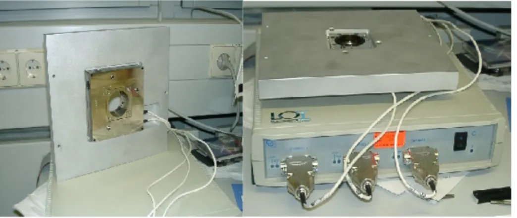
Figure 7: A typical scanning setup configuration.
3. MATERIALS AND METHODS
The time-resolved fluorescence scanner is based on an inverted microscope (Axiovert 100TV, Zeiss, Germany) equipped with a nanopositioning motion controller driven x,y,z-NPS 330 microscope scanning stage (max scanning volume 110 x 110 x 15 µm). Periodic wave motion and discrete positioning of the stage coordinates is accomplished through calls to a Windows 32 dll. The measurement routine was completely written in C to minimize time-consuming code overhead. As excitation source a pulsed diode laser emitting at 635 nm with a repetition rate of 64 MHz (PDL800;
Picoquant, Berlin, Germany) was used. The collimated laser beam passes trough excitation filters (for example: 630DF10; Omega Optics, Brattleboro, VT) and is directed to the microscope objective (for example: 100x, NA = 1.4, Olympus, Tokyo, Japan) by a dichroic beamsplitter (for example: 645DRLP; Omega Optics, Brattleboro, VT). The elliptical shape of the laser beam profile is then converted into a circular (Gaussian-like) profile by the use of two cylindrical lenses. The fluorescence light was collected by the same objective, filtered by a bandpass filter (for example: 675RDF50; Omega Optics, Brattleboro, VT) and directed through the TV outlet on the bottom of the microscope onto a pinhole oriented directly in front of either a single-photon avalanche photodiode (APD) or beamsplitters followed by more APDs (for example: SPAD, AQR-14, EG & G Optoelectronics, Canada). For the generation of fluorescence lifetime images of single molecules the signal of the avalanche photodiode was fed into a time-correlated single- photon counting (TCSPC) PC interface card (SPC-630, Becker & Hickl, Berlin, Germany) to acquire time-resolved data. With this card a minimum collection time of 150 µs per decay curve (64 channels) for a gap-free measurement is possible (Becker 1999).
For synchronization of the scanning motion with the detection device a Windows 32 based software with Microsoft Visual C++ 6.0 running under Windows 2000 was developed. The triggering of the detection device and data acquisition is done through calls to a Windows 32 dll (Becker & Hickl, Berlin, Germany). Within the routine, the
Windows data storage is done in binary format without system cache to avoid arbitrarily giving control to the operating system.
3.1. QUEENSGATE NPS3330
The Queensgate nanopositioning table is capable of scanning micrometer volumes at nanometer precision. The total possible scanning dimensions possible of the Queensgate table is 170*170*15 micrometers. Total linearity error is less than .02% and positional noise level is less than .005 nm/sqrt(Hz) (Xu, Atherson et al.; Xu, Atherson et al.). The table possesses linearity errors less than 0.01% is possible in reduced scan ranges. It possesses a positional noise less than .005 nm/Hz^2 (RMS). The table positions itself by applying a voltage to a piezocrystal and monitored by a capacitance sensor which in feedback minimize the wanted and actual positions of the table. Precision then is determined from resolution/noise (from the piezo, sensor, mechanical and acoustic), drift/hysteresis and mapping errors. The piezo system is non-linear so that up to a 4th degree order polynomial correction function is used to compensate for the tables physical/electrical properties. Adjusting the stiffness of the table can reduce ground vibration and acoustical noise effects. Angular motion errors can occur when specimens are mounted on the table. To reduce this specimens should be placed as close as possible to the measuring axes of the sensors. Dimensional changes in material used are determined from their coefficient of thermal expansion (CTE) so materials with low CTE such as Super Invar or Zerodur are used. Positional errors from thermal expansion and the position drivers have been decoupled. A Super Invar stage of 100*100 mm experiences a 30nm change in dimension from a 1° chance in temperature. Stress properties of the materials are also considered.
Figure 8: A scan of a part of a 100-µm-scale slide.
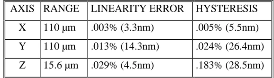
AXIS RANGE LINEARITY ERROR HYSTERESIS X 110 µm .003% (3.3nm) .005% (5.5nm) Y 110 µm .013% (14.3nm) .024% (26.4nm) Z 15.6 µm .029% (4.5nm) .183% (28.5nm)
Table 1: The Queensgate table used has been tested and the following results are available.
The Queensgate table allows for programmable periodical motion along any of the three axes. Periodic motion is used on one axis, this is because the maximum period allowed for an axis is 5.35 seconds, at an average of 5ms per pixel, this would allow for only 1070 pixels to be scanned in this time which would correlate to a 32*32 pixel domain in 2D which is to small for the average sized domains we examined. The other two axes were discretely positioned using software commands. The periodical curves possible include ramp, sin, square and sawtooth.
The first wavetype tested was the sin wave. The scanned domains produced using the sine type waveform need retransformations to Cartesian type projections. Although the transformation is possible, it is no longer possible to query individual pixels after the transformation is finished. Due to the uniform speed of the sine wave, more photons are collected near the x-boundaries and fewer in the inner domain, which result in further post-graphical corrections.
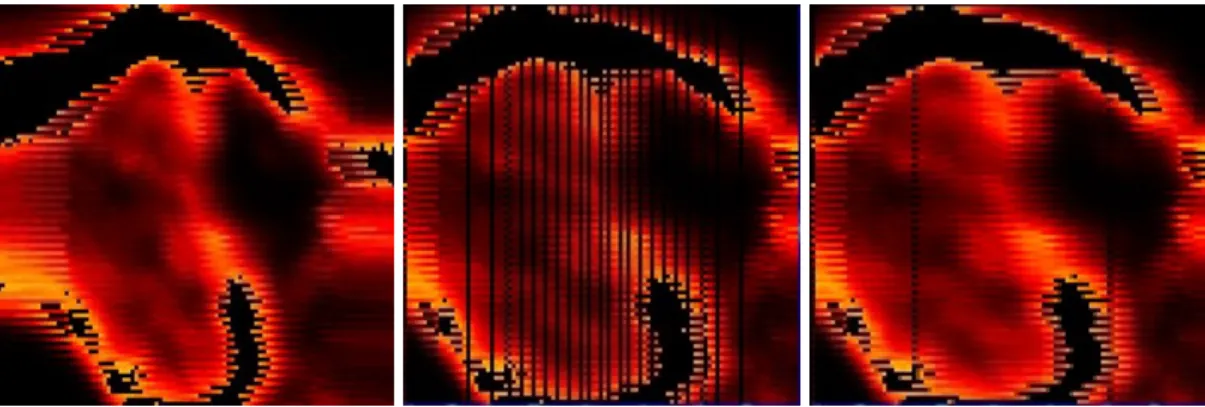
Figure 9: Left to right: Scans using the sine waveform used for the x-direction, corrected position and fill-in. The y-axis (top to bottom) lines have a zigzag quality due to small delays in y stepping. Although the image can be corrected information of the individual pixels is not uniform.
Figure 10: Same 10*10 micron scan using sawtooth waveform.
Rampwave motion was chosen as the favorite as it results in clear pictures that needed little further corrections. Also much information is lost after sin corrections in the image. Using periodical rampwave movement in the x-direction while the y/z movement was stepped performs actual three-dimensional measurements. This results in a set of two-dimensional scans.
Figure 11: The Queensgate nano positioning device NPS3330 XYZ
Internal inertia of the specimen (and the slide) resulted in unwanted movement so that limits on the speed of the periodical movement were needed.
3.2. SPC 630
A highly sensitive single photon avalanche diode (SPAD) detector together with a SPC-630 card allow for time-correlated single photon counting. The card can be made to run in several modes. Of these the FIFO mode can be used to collect the raw time data of incoming photons. This can be useful to find single molecules or to measure the time it takes to bleach the fluorescent dye. Another mode is the (continuous) scanning mode.
Here the information from a single decay of given collection time period is partitioned into to several channel bins. A photon signal depending on its arrival time is summed into one of these bins and forms the decay profile of the molecule scanned. Decays are stored on on-board blocks. When a block is full, the datablock is freed to be saved and reading continues into the next datablock. The SPC card also allows simultaneous collection of photon signals arriving from one or more SPD detectors using a raster.
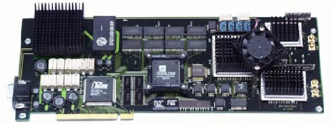
Figure 12: SPC630
Time-Correlated Single Photon Counting (TCSPC) is a technique to record low- level light signals with picosecond time resolution. Time-Correlated Single Photon Counting is based on the detection of single photons of a periodical light signal, the measurement of the detection times of the individual photons and the reconstruction of the waveform from the individual time measurements. The method makes use of the fact that for low level, high repetition rate signals the light intensity is usually so low that the probability of detecting one photon in one signal period is much less than one. Therefore, the detection of several photons can be neglected and the principle shown in the figure below can be used: The detector signal consists of a train of randomly distributed pulses due to the detection of the individual photons. There are many signal periods without photons; other signal periods contain one photon pulse. Periods with several photons are very rare. When a photon is detected, the time of the corresponding detector pulse is measured. The events are collected in memory by adding a ‘1’ in a memory location with an address proportional to the detection time. After many photons the histogram of the detection times, i.e. the waveform of the optical pulse, builds up in the memory.
Although this principle looks complicated at the first glimpse, it is very efficient and accurate for the following reasons: The accuracy of the time measurement is not limited by the width of the detector pulse. Thus, the time resolution is much better then with the same detector used in front of an oscilloscope or another linear signal acquisition device.
Furthermore, all detected photons contribute to the result of the measurement.
When a photon is first detected by a SPAD, a signal is sent to the constant fraction discriminator (CFD) of the SPC-card. Signals arriving are not square waves (for each photon), but a statistical wave due to the electronics involved. This means two identical photons with identical characteristics can be transformed into two different incoming signals. The goal then is to decide on a consistent method of determining the arrival time of the photon pulse. The CFD unit receives a signal and recombines an inverted and delayed part of this signal to create a zero crossing point that determines a consistent trigger time for the TAC.
Figure 13: The CFD adds a part of the inverted signal to the original signal to form a consistent temporal location of the detected photon pulse.
The time to amplitude converter (TAC) is composed of a ramp generator that is started by a trigger signal generated by the CFD. The ramp curve is stopped by a SYNC signal from the laser. The TAC is not started by the SYNC because the photons available are less than the pulses and we want the SPC to be ready to ‘work on’ the arrived photon.
If the TAC is started by the SYNC, the card may be active even when no photons are detected. During this activity no further photons can be detected and since we only receive few photons this method would have an unwanted effect. When we know the laser pulse frequency the ADC unit can find the correct time. This is the inverse
measurement principle. A voltage, proportional to the ramp (detection time) is then amplified and sent to the ADC.
Figure 14: General principle of the TCSPC measurement using the SPC modules
Figure 15: The summation process of the SPC card to form a decay curve.
The analog digital converter (ADC) receives a voltage from the TAC and increments the memory address corresponding to the TAC-time by one. A histogram of this memory resembles a decay curve for a preset collection time period.
The memory of the SPC card can be adjusted to acquire decay resolutions from 6 to 12 bit accuracy. This results in histograms with 2(bit resolution)
channels of type short (two
bytes). The total amount of histograms that can be held in a bank is then 256*210 / 2(bit
resolution+1).
Bit resolution Channels Bytes Histograms in bank
6 64 128 2048
8 256 1024 512
10 1024 2048 128
12 4096 8192 32
Table 2: SPC memory allocation.
3.3. THE PROGRAM
Most of the time spend on this work was done programming, especially post processing. Microsoft’s Visual C was chosen because of its inherent speeds and ability to communicate quickly with the hardware, moving large amounts of data from the SPC card to disk, with little (<5ms) delays. Also the Queensgate table and SPC card used came with windows dlls and libraries designed for use by a windows program.
3.3.1. The Scanning
Once the parameters for the measurement domain and photon collection parameters have been set the scanning is ready to initialize the Queensgate table and SPC card. The Queensgate table must be first initialized using an initialization file. The required waveform period is calculated by multiplying the collection time per pixel, the length of the x-axis and pixel resolution of the scanned domain and this parameter, multiplied by two, is sent to the Queensgate controller. If the time period exceeds a maximum 5.35-second limit for an axis, the collection time per pixel is modified so that this limit is employed. The dimensions of the domain to be scanned are checked to ensure that they are within the Queensgate scanning table’s bounds, otherwise the user is
informed to choose new settings. When all these conditions have been satisfied the scanning may begin.
The scanning first initializes a storage file and enough memory to hold the SPC's memory blocks. Since a scanning of a three-dimensional domain can result in large amounts of data (>200MB), blocks read from the SPC card are immediately saved to the storage file. This method avoids timing delays that could be a consequence of the operating systems memory handling.
The Queensgate operation is done as follows. The x-axis used with a periodical waveform is set at it initial position and waits there until a timed software routine triggers its start. This axis moves periodically defined by a waveform parameter until one two- dimensional plane has been scanned and then it is stopped and reset for the next z-plane if required. Software routines dependant upon the operating system’s timer controls the y- axis. The time interval between y-axis movements is equal to the collection time per pixel times the length of the x-dimension (in µm) times the pixels per µm resolution. Once an entire xy-plane has been scanned the z-axis is positioned and the xy-scanning restarts until all z-planes have been scanned.
Figure 16: Queensgate waveforms used for the x-axis. From left to right: ramp and square.
Scans using the rampwave option resulted in the clearest images being blurred only on one side due to measurements continuing during the resweep phase. Scans using the sawtooth wave possessed sub pixel blurring due to the y positioning delays at the edges.
The SPC card is initialized with various parameters that adjust themes discussed in section 5.2. At the start of a scan for a two-dimensional plane the SPC card is set in
continuous mode. In this mode, photon signal information is saved to one of the SPC’s block memory banks until it is full, then the SPC card immediately switches and uses its other memory bank. The SPC card sets an internal flag that is monitored by the software that signals one of its memory banks is ready to be read. This bank is then read and stored to a storage file. This memory bank is 524288 bytes large and is transferred in less time (average 83 ms on Windows 2000, x86 Family 6 model 5) than the time it takes to fill the other SPC block (collection time * number of curve data in SPC bank).
Figure 17: flowchart of scanning procedure
The flowchart in Figure 18 shows graphically how a scan is implemented. The timer for the yz movement is done in parallel with the SPC card tasks. The timer is triggered when the time for the x position completes one sweep. This can be calculated from the number of pixels per µm times the length in µm times the SPC photon collection time. Using this strategy allows the user to quickly scanning of large domains without unnecessary delays.
The program can be separated into two parts: scanning and postprocessing. For scanning a property sheet holds the entire property page dialogs associated with the scanning process.
In the cpp_SPC1 dialog, the user can choose how many detectors and what channel resolution to use. The SPC-card must be first initialized with an ini file to begin.
The program automatically loads an ini file to initialize the SPC card during the start of a measurement. If it cannot be found the user is asked where it is located. Although this is required from the SPC card, actual parameters are loaded from the previous values stored in the operating system’s registry. A user-defined ini file with preset values for the SPC parameter can be loaded here afterwards.
The user can set TAC, SYNC and CFD parameters of the SPC card in the cpp_SPC2 dialog. Various timing parameters (collection time, delay time, etc) of the SPC card can be adjusted in the cpp_SPC3 dialog. These settings define the photon monitoring explained in section 5.2.
The dialog cpp_SPC_pre is useful for adjusting the pulsed lasers intensity and cable length electronical modifications. The has a view window that monitors incoming photons for one second and displays the decay curve. An intensity window is also shown.
Using these windows as a graphical aid, one can adjust the SPC settings in dialog cpp_SPC2 and also the laser intensity without the need of additional monitoring devices.
Figure 18: SPC preview and adjustment dialog.
The main dialog for scanning is defined in cpp_QG2. The dimensions of the scanning area, as well as the pixel per micron resolution are set here. A small subroutine can aid in choosing a filename. If the user wishes, he can also create an ini-file for SPC- card usage for other programs.
Figure 19: The main scanning dialog.
For defining the communication ports of the Queensgate table, cpp_Qgsetup can be used. This dialog however is usually not needed since the Queensgate has its own set- up instructions. It is quite useful however when device conflicts are present.
The actual Queensgate positions can be viewed in the cpp_QGView1 dialog. This should be not used during scanning because the additional calls to this device increase the probability of synchronization errors. It is here only to verify that the Queensgate table is actually running and is utilizing the entire range. This is useful because various hardware configurations can prevent the actual wanted operational behavior.
3.3.2. Postprocessing
Data analysis is performed with a set of custom software tools written in C and C++. Lifetime information is calculated by a method based on the log-likelihood ratio estimator LL (Herten 2000).
1.
Here, ni is the number of photons acquired in each channel i running from 1 to k of the measured fluorescence decay and pi gives the modeled probability to detect a photon in the ith channel.
The graphical viewing options are adjusted in the d_Post dialog. One can set the graphical output to two or three dimensions. Output of intensity or lifetime data can be selected. Other options include rotation, transformation, opacity and zoom. In 3D-mode a cube may be included with the output as an orientation guide. In 2D an adjustable grid can be switched on. One may also decide to view certain xy-, xy- or yz-planes if desired.
In 2d mode the d_DecayViewModeless dialog can be invoked to show corresponding decay curve, intensity and lifetime details of the point under the current mouse position. The local channels used for lifetime estimations can be set by clicking the left mouse button, for minimum channel used, and the right mouse button for the maximum channel used. The user can choose auto scaling or manual to normalize the output. Auto scaling gives the best view of the decay whereas manual scaling can be better for viewing relative intensities. A logarithmic view is also possible.
In the d_postHistogram dialog, the local settings for intensities and detector lifetimes can be filtered using a histogram aid. It is often advisable to use this filter before changing from 2d to 3d viewing because of the amount of point memory that must be processed. For example one can over-filter a scan, leaving just a few reference points visible, then change into the 3d viewing mode, rotate to the desired position and then use the filter to reshow the filtered data.
Figure 20: Postprocessing Dialogs: a.) At the top the d_post general viewing settings, b) at the center is a histogram/filter dialog, c) to the center/right is the decay view: the left mouse selects the actual decay shown.
In the d_corrections dialog, it is possible to adjust the z-plane skewness. This may occur due to the internal inertia of the object and slide being examined. The motion of the Queensgate may cause them to drift. To avoid this, a weight can be placed on top of the slide under the microscope. Recently slide clips were built onto the Queensgate device.
However, it was found that the positions of the slide clips could affect the motion of the device. One could also increase the time per pixel option, but this leads to longer scanning times.
In the d_postgraphicparameters dialog it is possible to set the global min/max filter values for channels, lifetimes and intensities of the detectors used. The file is then reloaded with these filters and redisplayed. It is also possible to reset the settings to the original file attributes.
In 2d-mode, details of individual pixels or elliptical areas can be collected either individually, by pressing space, or grouped, by pressing ‘a’. The d_SnapGraphics dialog is used for viewing this data. One can choose to save the data in text or excel format. It is also possible to view fractional to lifetime plots (See Figure).
Figure 21: snapshots: give information about individual or a group of photons, such as detector counts, lifetimes, fractional intensity and total intensity.
Included in the dialog above is the D_Snapshot_modeless dialog. Fractional to lifetime data plots can be visualized here. These can be saved as bmp files. Fractional intensities can be calculated by dividing the number of photon arriving from a specific
detector by the total number of photons collected. For example, two detectors monitor intensities I1 and I2, the fractional part arriving from the second detector is then
F2 = I2/(I1+I2). 2.
This information can be used when the wavelength properties of the detectors is known to differentiate the signals arriving from a set of molecules.
Figure 22: Snapshot: here the fractional intensities (y-axis) are plotted against the lifetime values (x-axis). Fractional intensities can help a researcher determine if one or several objects are present and their distance from each other.
3.3.3. Miscellaneous Dialogs
A dialog to show the color scale used is available as well as a dialog that does a point-sum of all decays and displays this along with its lifetime approximation. There is
an information box giving details about the scanned file itself. This gives information from the file header. The information includes SPC information such as block length, blocks per page, maxblock number, collection time and the number of detectors. The Queensgate information provided includes the domain lengths, offsets and resolution as well as the waveform used for the first dimension.
The program can exports bitmap data of the main 2d and 3d screen output as bitmap and Davis img data as well as set the background screen of the Windows operating system.
In the post 2d viewing mode the program will monitor the mouse position if its left button is pressed and if so give information of the scanned position to the caption bar as well as the decayview if it is visible.
For 3d view an option allows the user to have the bitmap blow-up instead of the pixels. In 3d, individual pixels get spread wider apart as the viewing size increases.
Blowing the bitmap up first creates the bitmap at original size and expands this so those pixels become large squares.
To measure distances between two points in the 2d image, one presses the left mouse to select the first point and the right mouse button for the 2nd point. The distance will be then visible in the caption bar. An optional ruler can be shown and has 50 pixel knots for orientation purposes.
As a viewing aid, one can plot the image using grayscales and also show gradients. This can make visible hard to see details in the image.
3.3.3. The Visualization
Curve pixel data is first put through a user definable global filter and saves in an array of point objects that contain information about the position and intensity of the point. Lifetime information is dependent upon that curve resolution and calculated directly from the data file, as it is needed. Given the dimensions and resolutions of a scan, the point’s position can be stored to a single long variable. For example, the 3 coordinates, x, y, and z can be scaled to integer values. Each line has X points and each plane has XY points. So any point can be coded to x + y*X + z*XY, when x of 0..X-1, y of 0.. Y-1 and z of 0..Z-1.
The scanned domain is transferred to a unit cube (side length =1) and contains the origin at its center. Then, each of 3d points to the computer screen may require a 3d- tranformation, a 3d-rotation and finally a projection onto a two-dimensional monitor.
Adding a vector and applying matrixes to the point accomplish this and finally scaling the x/y coordinates with a function dependant on the z coordinate.
Here is the summary:
x=x+skewfactorX*z y=y+skewfactorY*z
X=X+Translation ; where X=(x,y,z)
W=A*X ; where A=rotations matrix
Factor1=z/d1+d2 ; d1, d2 “fish-eye” scaling factors, d2 should be chosen that Factor1 stays greater than 0.
Factor2=size/d screenX=x * Factor2
screenY=y * Factor2 * aspect ratio factor
4. EXAMPLES
4.1. A DEAD CELL
Figure 23: A scan of an old cell without a pinhole. The scan resulted with cylindrical objects.
Scans were preformed on old cancer cells. Initially no pinhole was used as part of the calibrating of the confocal microscopy setup. This resulted in cell objects appearing cylindrical due to the consequence of out of focus z-layers blurs.
Figures 24: Dead cells. From left to right: 80x80 microns, 40x40 microns, 20x20 microns, and 10x10x10 microns at 3 pixels/micron. Laser intensity was set at 20 µwatts and a 50-µm pinhole was used.
The pictures in Figure 25 shows the same set of cell scanned with the pinhole. The figures are a sequence of zooms of a single volume. The developed software enables the researcher to zoom in on selected areas with the computer mouse pointer and adjust resolution. This method saves time when searching for objects to scan.
4.2. BREAST CANCER
Figure 25: Scans from Thomas Heinlein: Small area, approximately 15x15x5 microns at 10 pixels/micron, laser intensity set to 20 µwatts. Breast cancer cells marked with antibodies attached to the membrane. This antibody is detected by a secondary antibody marked with a Bodipy 630/650 (IgG).
The Scans in Figure 26 were performed on Breast cells infected by cancer. By using the 3d feature of the software the researcher can view volumetric details such as
cellular interaction and relative positions. It is also possible here to quickly find a z- coordinate level for more detailed scanning in 2d.
5. DISCUSSION AND OUTLOOK
Scanning micrometer objects has been around for a while. The program can correctly identify single molecules with dyes attached to them with nanometer precision.
The program shows it is possible to produce high-resolution three-dimensional images in micrometer range. The signals originate from an elliptical measurement volume of 10-15 liters. Typical dye might need up to five ms to move through this volume at 10-6 cm2 /s resulting in a total detection volume of one micrometer. The laser used has a radius of 200-300 nanometers. Typical cells measured had a diameter of 600 nm. The laser then only excites a part of the cell. The pinhole further filters the resulting emission that enables higher resolution.
Figure 26: The measurement volume.
The program developed reveals new information concerning the 3D properties of molecules. Whereas in two dimensions one can observe and analyze fluorescent
behaviors of molecules, in three dimensions one can better view the actual volumetric properties of molecules, thereby revealing the sub micrometer structure and interactions among molecules and their environment.
The work further verifies the benefits of confocal microscopy. The resolution in 2D is restricted to approximately 500nm. The Figures 3, 6, and 24 were performed without a pinhole. These images reveal the effects of blurring from light scattering. Other Figures using the pinhole possess greater effective resolution, improved signal to noise.
The pinhole enables the measurements using the z-axis. Using 3d techniques developed in the work in combination with the pinhole researcher can examine thick specimens and gives a depth perception quality to the scanned images. The program developed reveals detailed information about the distribution of molecules 3D. For example, we found proteins used to mark a cell membrane to be also in the nucleus.
This program allows researchers to scan several layers of an object. This can benefit a researcher using 2d techniques by helping him to find certain z-levels of interest and allowing him to adjust the 3d nanopositioning table using software assistance.
Future enhancement of this and program like this one are mostly limited by computational power and the features of the measurement hardware. The Queensgate 3d nanopositioning table for instance has a 5.35 second limit for any of its axes. Although the positioning accuracy of the resulting images is very high, this involved special attention given to the timing routines that control the data transfers and axis positioning.
Also beneficial could be the implementation of user defined periodical curves for the 3d tables axes. It would also be nice if the SPC-630 photon detection card could posses more memory. This, in combination with longer axes periods, could allow scans of large volumes or high resolution that require large sums of memory to be scanned completely
to the photon detection cards memory with a minimal of software communication or operating system interrupts.
APPENDICES
A. INDEX OF ABBREVIATIONS
ADC Analogue to Digital Converter AFM Atomic Force Microscopy APS 3-Aminopropyl-triethoxysilane ATP Adenosine Triphosphate
bp base pairs
CCD Charge Coupled Device
CFD Constant Fraction Discriminator DCTP 2’-Deoxycytosine-5’-triphosphate ds double-stranded
dUTP 2’-Deoxyuridin-5’-triphosphate DNA Deoxyribonucleic Acid
EOM Electro-Optical Modulator FCS Fetal Calve Serum
FIFO First-In-First-Out
FLIM Fluorescence Lifetime Imaging Microscopy FRET Fluorescence Resonance Energy Transfer FWHM Full Width Half Maximum
GFP Green Fluorescent Protein
HOMO Highest Occupied Molecular Orbital IC Internal Conversion
IRF Instrument Response Function ISC Intersystem Crossing
LASER Light Amplification by Stimulated Emission of Radiation LH Light Harvesting
LIF Laser-Induced Fluorescence
LS Least Squares
LUMO Lowest Unoccupied Molecular Orbital
ML Maximum Likelihood
MLE Maximum Likelihood Estimator MCS Multi-Channel Scalar
NA Numerical Aperture
NADH Nicotinamide Adenine Dinucleotide NSOM Near-field Scanning Optical Microscopy PC Personal Computer
PCR Polymerase Chain Reaction PGA Programmable Gain Amplifier PMMA Poly (methyl methacrylate) PSF Point Spread Function PVA Poly (vinyl alcohol) PVP Polyvinyl pyrolidone
RS-232 Recommended Standard No. 232 S/B Signal-to-Background
SERS Surface Enhanced Raman Spectroscopy
SFLIM Spectrally-resolved Fluorescence Lifetime Imaging Microscopy SMD Single Molecule Detection
SMS Single Molecule Spectroscopy S/N Signal-to-Noise ratio
SPAD Single Photon Avalanche Diode SPC Single Photon Counting
ss single-stranded
STED Stimulated Emission Depletion SYNC Synchronization
TAC Time-to-Amplitude Converter
TCSPC Time Correlated Single Photon Counting
B. THE SCANNING ROUTINES
void cpp_QG2::_levelmeasure()//3d scan = several 2d scans {
bxzdone=false;
bsomething=false;
mupy=(int)qg_command->m_muy*qg_command->m_py;
int mupx=(int)qg_command->m_mux*qg_command->m_px;
int npoints=mupx*mupy;
ncycle=npoints/SPC->mem_info.maxpage+1;//4096 SPC_set_parameter( COLLECT_TIME, m_collect_time );
SPC->iMeasurementInProcess=m_idatasaved=1;
SPC_set_page( 0 );
SPC_enable_sequencer( 1 );//continuous mode SPC_set_parameter( MEM_BANK, 0 );
SPC_fill_memory(-1, -1 , 0);
SPC_set_parameter( MEM_BANK, 1);
SPC_fill_memory(-1, -1 , 0); // clear bank DYIELD;
short spc_state=0;
short armed;
int cycle;
int nok;
float mbank;
float d_ytime,d_xytime;
m_nwrites=0;
mbank=0.f;
SPC_set_parameter( MEM_BANK, mbank);
//the timer steps the y-axis
//which steps the z-axis if neccessary.
d_ytime=m_collect_time * 1000.0f *
qg_command->m_mux *qg_command->m_px;
d_xytime=d_ytime*qg_command->m_muy*qg_command->m_py;
cycle=0;
Timed_X_move_init();//_levelmeasure
if(SetTimer(5, (int)(d_ytime/2),NULL)==0){AfxMessageBox ("Timer 5 could not be initialized, restarting" );OnGo();}//check if while(armed) loop took time
if(SetTimer(6, (int)(d_xytime),NULL)==0){AfxMessageBox ("Timer 6 could not be initialized" );OnStop();} //plane time
////////////start timer and wave at same time///////////////////////////////////////////////////////
if(SetTimer(3, (int)(d_ytime), NULL)==0){AfxMessageBox ("Timer 3 could not be initialized" );OnStop();} //y time
qg_command->continuewave(1);//start the x wave //////////////// LOOP ///////////////////////////////////////////////////
do{ //get data from SPC
// Well always start the SPC and stop it manually nok=SPC_start_measurement();
////==============================================
armed=1;
while(armed){
SPC_test_state( &spc_state );
DYIELD;
if(istop==1){Stop();return;}//user stop if(( spc_state & SPC_ARMED )==0){
armed=0;
//SPC_read_gap_time(&last_gap);
}
if( bxzdone)armed=0;
} //while(armed)
////==============================================
if (bsomething==false){
OnStop() ; OnGo();
}
#ifdef readpage // read current bank: SPC6** //not for SPC3*0
#ifdef hugememory //._levelmeasure
if(bhuge){//read to computer memory if(!bfastnsmall){
int i=m_nwrites*SPC->mem_info.maxpage //*sizeof(unsigned short)
*SPC->mem_info.block_length
*SPC->mem_info.blocks_per_frame;
m_ierr=SPC_read_data_page(0, SPC->mem_info.maxpage-1,
&jfile->pnDataPage[i] );
}
}else{ //<.005s/pixel & >4096 pixels //not used m_ierr=SPC_read_data_page(0,
SPC->mem_info.maxpage-1,
jfile->pnDataPage );//not for SPC3*0 }
#else
m_ierr=SPC_read_data_page(0,SPC->mem_info.maxpage-1,jfile-
>pnDataPage );//not for SPC3*0
#endif
#endif //readpage
if(!bfastnsmall)
SPC_fill_memory(-1, -1 , 0);//fills mbank block if(!bhuge){
jfile->dwPageSize=SPC->mem_info.maxpage ;//rest jfile->dwPageSize*=sizeof(unsigned short);
jfile->dwPageSize*=SPC->mem_info.block_length; //64 jfile->dwPageSize*=SPC->mem_info.blocks_per_frame;
jfile->writefile(jfile->pBuffer,jfile->dwPageSize );///critical }
m_nwrites++;
#ifndef hugememory //_levelmeasure
sprintf(s,"Writing Block %i",m_nwrites); //
AfxMessageBox ( s);
#else
sprintf(s,"Vriting Block %i",m_nwrites); //
AfxMessageBox ( s);
#endif
GetDC()->TextOut (10,5,s);
DYIELD;
//}//cycle
}while (++cycle<ncycle);
//////////////////////////////////////////////////////////////////////////
}
void cpp_QG2::_levelinitpositions()
{//called when z changed by timed_y_move // stops and saves data
// moves z
SPC_stop_measurement();
KillTimer( 3 );
KillTimer( 4 );
SPC_enable_sequencer(0);// turn off photon counting SPC->iMeasurementInProcess=0;
qg_command->StopWave(1);
if(m_nwrites!=ncycle-1)return;
// READ THE DATA FROM SPC ///////////////////////////////////////////
#ifdef hugememory //_levelinitpositions if(bhuge){
if(bfastnsmall){//fast scan completely in SPC memory float mbank;int i=0;
if((decays==SPC->mem_info.maxpage)|| //if sequenser on (decays==2*SPC->mem_info.maxpage))
{
SPC_get_parameter( MEM_BANK, &mbank);
mem_bank=mbank?(short)0:(short)1;
SPC_set_parameter( MEM_BANK, mem_bank);
}
if(decays>SPC->mem_info.maxpage){
//AfxMessageBox ( "SPC mem save");
SPC_get_parameter( MEM_BANK, &mbank);
mem_bank=mbank?(short)0:(short)1;
SPC_set_parameter( MEM_BANK, mem_bank);
m_ierr=SPC_read_data_page(0,
SPC->mem_info.maxpage-1, jfile->pnDataPage );
mem_bank=mbank?(short)0:(short)1;
SPC_set_parameter( MEM_BANK, mem_bank);
i=SPC->mem_info.maxpage
*SPC->mem_info.block_length
*SPC->mem_info.blocks_per_frame;
}
m_ierr=SPC_read_data_page(0,SPC->mem_info.maxpage-1,
&jfile->pnDataPage[i] );
}else{//>.005s
//sprintf(s,"SPC normal mem save %i",m_nwrites);
AfxMessageBox ( s);
m_ierr=SPC_read_data_page(0,SPC->mem_info.maxpage-1,
&jfile->pnDataPage[m_nwrites
*SPC->mem_info.maxpage //*sizeof(unsigned short)
*SPC->mem_info.block_length
*SPC->mem_info.blocks_per_frame] );
}
}else{//<.005s/pixel & >4096 pixels //not used
SPC_read_data_page(0,SPC->mem_info.maxpage-1,jfile->pnDataPage );//not for SPC3*0
}
#else
SPC_read_data_page(0,SPC->mem_info.maxpage-1,jfile->pnDataPage );//not for SPC3*0
#endif
// SAVE THE DATA TO DISC //////////////////////////////////////////
int mupxmupy=(int)qg_command->m_muy*qg_command->m_py
*(int)qg_command->m_mux*qg_command->m_px;
DWORD dwPageSize;
//#ifdef hugememory //_levelinitpositions if(bhuge)
dwPageSize=mupxmupy;//greater than block size else
//#else
if(mupxmupy<= SPC->mem_info.maxpage )//save b4 spc block full dwPageSize=mupxmupy;
else // 1st part of plane saved by _levelmeasure
dwPageSize=mupxmupy % SPC->mem_info.maxpage ;//rest //#endif
dwPageSize*=sizeof(unsigned short);
dwPageSize*=SPC->mem_info.block_length; //64 dwPageSize*=SPC->mem_info.blocks_per_frame;
jfile->dwPageSize = dwPageSize;
jfile->writefile(jfile->pBuffer,dwPageSize );
m_nwrites++;
sprintf(s,"Writing block %i",m_nwrites); // AfxMessageBox ( s);
GetDC()->TextOut (10,0,s);
// sprintf(s,"size %i",dwPageSize); // AfxMessageBox ( s);
// GetDC()->TextOut (10,16,s);
// PREPARE TO SCAN NEXT LEVEL NOW /////////////////////////////
// move QG:Y
Timed_Y_move_init();
// move QG:Z izz++;
int mupz=(int)qg_command->m_muz*qg_command->m_pz;
if(izz<=(mupz-1)) {
float fz=fzz;
if(mupz>1)fz+=(float)izz*(qg_command->m_muz/(float)(mupz-1));
qg_command->setZposition(fz);
int nChannel = 3;float fz1;
do{
Read_Measured_Position_F( &qg->m_nController, &nChannel,
&fz1 );
qg_command->setZposition(fz);
// MessageBeep(-1);
//char s[80];sprintf(s,"%f %f", fz,fz1);
AfxMessageBox ( s);
}while (fabs((double)(fz-fz1))>.5);
sprintf(s,"-> %i z=%5.3f ", izz,fz); // AfxMessageBox ( s);
CDC *pDC=GetDC();
pDC->TextOut (250,0,s);
//char s[80];sprintf(s,"%f %f %f", fzz,fz,(float)qg_command->m_pz);
AfxMessageBox ( s);
_levelmeasure();
ReleaseDC(pDC);
} //
else{
jfile->closefile();
EnableButtons(TRUE);
*iscanned=1;//_levelscan Stop();
} }