Supplementary Tables and text
Supplementary tables
Table S1 – Estimates of null allele frequencies for each locus obtained with Dempster’s EM method [1]. Confidence intervals are given.
Locus Frequency Estimate 2.5% 97.5%
CT77 0.0931 0.0698 0.1192
CT68 0.0247 0.0102 0.0448
CA58 0.0720 0.0546 0.0931
CT87 0.0712 0.0487 0.0977
AjTR-37 0.0364 0.0189 0.0590
CA55 0.0722 0.0380 0.1179
CT59 0.0875 0.0652 0.1131
CT76 0.0521 0.0320 0.0763
CT53 0.0100 0.0000 0.0326
CT89 0.0413 0.0226 0.0641
CA80 0.1283 0.1050 0.1543
CT82 0.0292 0.0135 0.0496
I14 0.0359 0.0178 0.0587
AjTR-27 0.1708 0.1394 0.2039
O08 0.0255 0.0080 0.0487
M23 0.0629 0.0319 0.1003
AjTr-45 0.1629 0.1356 0.1935
C01 0.0567 0.0247 0.0948
N13 0.1016 0.0774 0.1287
B22 0.1601 0.1322 0.1909
AjTr-42 0.1654 0.1370 0.1965
B09 0.1167 0.0930 0.1441
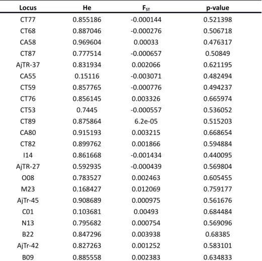
Table S2 - Neutrality test on microsatellite data
Locus He FST p-value
CT77 0.855186 -0.000144 0.521398
CT68 0.887046 -0.000276 0.506718
CA58 0.969604 0.00033 0.476317
CT87 0.777514 -0.000657 0.50849
AjTR-37 0.831934 0.002066 0.621195
CA55 0.15116 -0.003071 0.482494
CT59 0.857765 -0.000776 0.494237
CT76 0.856145 0.003326 0.665974
CT53 0.7445 -0.000557 0.536052
CT89 0.875864 6.2e-05 0.515203
CA80 0.915193 0.003215 0.668654
CT82 0.899762 0.001866 0.594884
I14 0.861668 -0.001434 0.440095
AjTR-27 0.592935 -0.000439 0.569804
O08 0.783527 0.002463 0.605455
M23 0.168427 0.012069 0.759177
AjTr-45 0.908689 0.000975 0.561676
C01 0.103681 0.00493 0.684484
N13 0.795682 0.000754 0.569096
B22 0.847296 0.003938 0.68385
AjTr-42 0.827263 0.001252 0.583101
B09 0.885558 0.002383 0.634833
FST / expected heterozygosity (He) relationship as well as p-value assuming neutral evolution in an island model with migration and considering 9 populations. * denotes significant p-values (0.05) suggesting positive or balancing selection.
Table S3 – Results of demographic analyses on microsatellites
2010 2011 2012
Matriline A B C A B C A B C
Allele frequency
class
Frequencies
0.1 0.789 0.738 0.742 0.797 0.736 0.711 0.780 0.738 0.734
0.2 0.137 0.169 0.164 0.129 0.155 0.180 0.143 0.167 0.154
0.3 0.033 0.048 0.049 0.031 0.081 0.066 0.040 0.048 0.066
0.4 0.020 0.020 0.020 0.017 0.000 0.013 0.017 0.024 0.025
0.5 0.003 0.008 0.008 0.010 0.016 0.009 0.007 0.004 0.004
0.6 0.007 0.000 0.000 0.003 0.000 0.009 0.000 0.008 0.004
0.7 0.000 0.004 0.004 0.000 0.000 0.000 0.003 0.000 0.000
0.8 0.000 0.000 0.000 0.000 0.000 0.000 0.000 0.000 0.000
0.9 0.000 0.000 0.000 0.000 0.000 0.013 0.007 0.000 0.008
1 0.010 0.012 0.012 0.010 0.012 0.000 0.003 0.012 0.004
Probability
H deficiency
0.5000
0 0.61274 0.67218 0.30508 0.84735 0.78776 0.25142 0.71697 0.38726
Probability
H excess
0.5126
9 0.39952 0.33943 0.70604 0.16044 0.22170 0.75870 0.29396 0.62488
Probability H excess or deficiency
1.0000
0 0.79903 0.67886 0.61015 0.32088 0.44341 0.50284 0.58793 0.77453
Frequency distribution
Normal L-shaped
Normal L-shaped
Normal L-shaped
Normal L-shaped
Normal L-shaped
Normal L-shaped
Normal L-shaped
Normal L-shaped
Normal L-shaped on allele frequency shifts and heterozygote excess/deficiency of each deme within cohorts Wilcoxon probability tests were made to test for heterozygote deficiency, excess (one tail test) and for excess or deficiency (two tail tests). Significant comparisons are marked with *. BOTTELNECK runs were performed (Cornuet & Luikart 1996) performed under a two-phase model of evolution (TPM), considering a 10% stepwise mutation and a 10%
variance for the TPM.
Table S4 – FST values for mtDNA (below diagonal) and microsatellites (above diagonal) considering the 9 demes.
A2010 B2010 C2010 A2011 B2011 C2011 A2012 B2012 C2012
A2010 0 0.001 0.003 0.003 0.005** 0,003 0,002 0,004 0,002
B2010 0,704** 0 0,001 0,002 0,004 0,001 0,001 0,000 0.003
C2010 0.577** 0.542** 0 0.004 0.005 0.001 0.001 0.000 0.003
A2011 -0.003 0.638** 0.501** 0 0.004 0.003 0.004* -0.002 0.003
B2011 0.714** -0.012 0.563** 0.648** 0 0.000 0.005* 0.004 0.007*
C2011 0.574** 0.533** 0.012 0.492** 0.555** 0 0.001 0.000 -0.002
A2012 -0.005 0.682** 0.550** -0.001 0.691** 0.543** 0 0.002 0.000
B2012 0.727** -0.004 0.582** 0.660** -0.003 0.573** 0.704** 0 0.006
C2012 0.554** 0.500** -0.011 0.475** 0.520** 0.007 0.521** 0.534** 0
* and ** denotes p-values significant for 0.05 and 0.01 (after correction for false discovery rate (Narum 2006).
Noteworthy, the high values of mtDNA are a by-product of the separation of the samples based on mtDNA haplotypes, and were only calculated to investigate the relationship between mitochondrial and nuclear genetic differentiations.
Table S5 – Outputs of the four-step process following Evanno et al to calculate ΔK [2].
# K Reps Mean LnP(K) Stdev LnP(K) Ln'(K) |Ln''(K)| Δ K
1 5 -33122,5 0,7246 NA NA NA
2 5 -33592,62 36,8153 -470,12 447,42 12,153096
3 5 -33615,32 126,9436 -22,7 534,02 4,20675
4 5 -34172,04 129,0306 -556,72 1026,98 7,959196
5 5 -33701,78 81,7719 470,26 657,74 8,043598
6 5 -33889,26 414,23 -187,48 163,18 0,393936
7 5 -33913,56 374,8048 -24,3 61,1 0,163018
8 5 -33876,76 389,9178 36,8 36,46 0,093507
9 5 -33803,5 416,5669 73,26 NA NA
Table S6 - Estimates for the modes and respective 95% confidence interval for mutation-scaled effective population size (θ) and Nem in model II, where 4Nem=Mj->i*θ for 2010
Parameter mode 2.50% 97.50%
A 0.067 0 3.867
B 2.067 0 5.2
C 2.467 0 5.867
Nem B A 0.325 0 9.167
Nem C A 0.318 0 9
Nem A B 10.161 0 9.167
Nem C B 8.095 0 9.167
Nem A C 11.716 0 9
Nem B C 9.661 0 7.667
Table S7 - Estimates for the modes and respective 95% confidence interval for mutation-scaled effective population size (θ) and Nem in model II, where 4Nem=Mj->i*θ for 2011
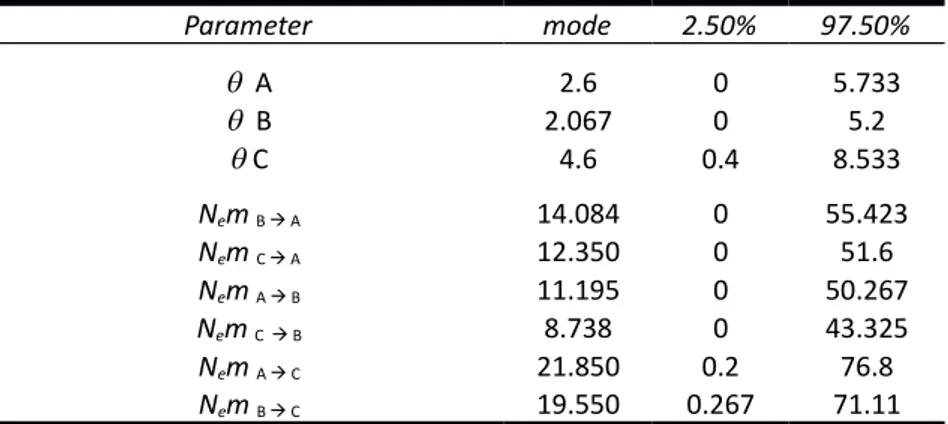
Table S8 - Estimates for the modes and respective 95% confidence interval for mutation-scaled effective population size (θ) and Nem in model II, where 4Nem=Mj->i*θ for 2012.
.
Parameter mode 2.50% 97.50%
A 2.6 0 5.733
B 2.067 0 5.2
C 4.6 0.4 8.533
Nem B A 14.084 0 55.423
Nem C A 12.350 0 51.6
Nem A B 11.195 0 50.267
Nem C B 8.738 0 43.325
Nem A C 21.850 0.2 76.8
Nem B C 19.550 0.267 71.11
Parameter mode 2.50% 97.50%
A 0.067 0 113.33
B 0.067 0 126.67
C 4.2 0.667 145.07
Nem B A 0.295 0 28.333
Nem C A 0.328 0 31.668
Nem A B 0.295 0 48.357
Nem C B 0.195 0 29.155
Nem A C 20.650 0.333 72.2
Nem B C 12.250 0 51.933
Supplementary text:
1. Amplification and genotyping of microsatellite loci
Amplification took place in four PCR multiplexes of four to six loci. Specifically, multiplex A – annealing 55°C (CT77; CT87; CA55; CA58; CT68; AJTR-37), multiplex B - annealing 55°C (CT82; CT76; CT89; CT59; CA80; CT53), multiplex C - annealing 60°C (C01; M23; AJTR-45; AJTR27; I14; O08), multiplex D - annealing 60°C (AJTR-42; B09;
B22; N13). All reactions were performed in a total volume of 10 μl and followed the QIAGEN© Multiplex PCR kit’s recommendations. Genotyping was performed on an ABI© 3100 Genetic Analyzer. Alleles were called in GENEMARKER© v. 1.91 (Softgenetics LLC, State College, PA).
Supplementary References
![Table S1 – Estimates of null allele frequencies for each locus obtained with Dempster’s EM method [1]](https://thumb-eu.123doks.com/thumbv2/1library_info/5346767.1682376/1.892.241.642.354.877/table-estimates-allele-frequencies-locus-obtained-dempster-method.webp)