RETRIEVING PATTERNS OF GENETIC DIVERSITY IN A GLOBAL SET OF CHICKEN BREEDS
Dissertation submitted
to obtain the Doctor of Philosophy (Ph.D) degree at the Faculty of Agricultural Sciences, Georg-August-University Göttingen, Germany
Presented by
Dorcus Kholofelo Malomane Born in Bushbackridge, South Africa
Göttingen, September 2019
D7
Reference 1: Prof. Dr. Henner Simianer Reference 2: Prof. Dr. Steffen Weigend Reference 3: Prof. Dr. Armin Otto Schmitt
Day of disputation: 08 November 2019
TABLE OF CONTENTS
SUMMARY 5
ZUSAMMENFASSUNG 9
CHAPTER 1 General introduction 13
The origin of chicken 14
From centers of domestication in Asia to the world: a
brief history of chicken dispersion 15
Main categories of breeds forming the global chicken
diversity 17
Acquisition and use of genomic data for genetic
diversity studies 19
The high density SNP genotyping array for chicken 20 SNP annotation and functional classification 21 Model for the cause of genetic differentiation between
populations 24
A single founder migration model of genetic diversity 24 Measures of genetic diversity and population structure 25
The aim and objectives 27
CHAPTER 2 Efficiency of different strategies to mitigate ascertainment bias when using SNP panels in
diversity studies 35
CHAPTER 3 The SYNBREED chicken diversity panel: A global resource to assess chicken diversity at high genomic
resolution 79
CHAPTER 4 Genetic diversity in global chicken breeds as a
function of genetic distance to the wild populations 121
CHAPTER 5 General discussion 167
The effects of ascertainment bias on genetic diversity
estimates 168
Correcting for ascertainment bias 171 The SYNBREED chicken diversity panel (SCDP) and
data availability 173
The applicability and limitations of the ‘single founder
migration model’ in domesticated chicken 177
Main conclusions 179
APPENDIX 185
SUMMARY
The chicken was first domesticated about 6000 B.C in Asia. Today the species is widely spread across the globe providing a good source of quality protein. There have been concerns about the loss of genetic diversity within the species due to the rapid spread and domination of the highly intensive commercial lines which utilizes small number of breeds with limited genetic diversity.
In addition, a strong phenotypic selection for fancy breeds which has become very popular in the 19th century has affected the genetic diversity of many populations. Genetic diversity in a population or a species is very important for its fitness e.g. adaptations to changing environments and resistance to diseases. Therefore, it is important to preserve the genetic resources in the chicken for its sustainability and to be able to respond to unforeseen circumstances. Genetic diversity studies are crucial in order to make informed decisions for the conservation and effective management of farm animal genetic resources.
Our study was focused on investigating the genetic diversity in a global set of chicken breeds based on the SYNBREED chicken diversity panel (SCDP). The SCDP consists of a total of 174 chicken populations from Asia, Europe, Africa and South America, which were genotyped with the 600K Affymetrix® Axiom™ HD Genotyping Array for chicken comprising of 580,961 SNPs. The panel includes two wild populations (Gallus gallus gallus and Gallus gallus spadiceus), 12 commercial lines (4 brown egg layers, 4 white egg layers and 4 broilers), 81 local breeds, and 79 fancy breeds of European and Asian backgrounds. Given the sensitivity of SNP data to ascertainment bias, we first investigated how we can mitigate the effects of ascertainment in our data when studying the genetic diversity.
In chapter 2 we used 42 of the 174 populations from our data which had both individual genotype data as well as pool whole genome resequencing (WGS) data. We estimated various genetic diversity measures i.e. expected heterozygosity (𝐻𝑒), fixation index (𝐹𝑆𝑇) values, phylogenetic analysis and principal components analysis (PCA), using the SNP array and WGS data, and compared the results. The array data overestimated the 𝐻𝑒, underestimated the pairwise 𝐹𝑆𝑇 values between breeds which had low 𝐹𝑆𝑇 values (<0.25) in the WGS data, and overestimated 𝐹𝑆𝑇 values (>0.25) for high WGS 𝐹𝑆𝑇. The PCA and phylogenetic analysis were less affected by ascertainment bias. Subsequently, we applied different SNP filtering options such as SNPs polymorphic in the Gallus gallus (founder populations), linkage disequilibrium (LD) based pruning and minor allele frequency (MAF) filtering and the combinations thereof to the array data. Then we assessed the option/s that could account for the ascertainment bias effects and were therefore viable to improve the accuracy of subsequent studies. Generally, the LD based pruning of SNPs produced better results which were comparable to the WGS. The overestimation of 𝐻𝑒 was slightly reduced and 𝐹𝑆𝑇 values were a little lower than in the WGS data, but in a systematic manner.
We performed the LD based pruning of SNPs to the array data for further genetic diversity analyses in chapters 3 and 4. In chapter 3 we studied the overall genetic diversity within and between the chicken populations. PCA and admixture analysis showed a continuous separation of Asian breeds at one end and European breeds on the other. The African and South American breeds clustered mostly in between but slightly towards either the Asian or the European cluster, supporting their Asian and European backgrounds of origin. The commercial white layers clustered towards European breeds and the brown layers and broilers clustered with the Asian breeds, reflecting their parental backgrounds. Furthermore, the fancy breeds covered a wide spectrum of the genetic diversity and clustered with other breeds of similar origin. However, the fancy breeds and the
highly selected commercial layer lines showed low genetic diversity within population with average observed heterozygosity lower than 0.205 across breeds’ categories. The wild and less selected African, South American and some local Asian and European breeds showed high within population genetic diversity with the average observed heterozygosity greater than 0.225.
In chapter 4 we further investigated if the observed overall genetic diversity within the populations in chapter 3 is a consequence of their genetic expansion from the wild populations.
We studied this following the single founder migration model which asserts that the genetic diversity within populations decreases with the increase in geographic distances from their founders. Additionally, as a consequence of the geographic expansion, genetic differentiation is expected to increase between the populations and the founder population. In our study we didn’t have geographic distances and the geographical location of the sampling in chicken often does not coincide with the geographical location of the breed development. Therefore, we used the Reynolds’ genetic distance of the sampled breeds to the wild ancestors as a proxy for geographic distance, and verified, whether the reduction of diversity can also be found with increasing genetic distance to the domestication center. We found that 87.5% of the variation in the overall genetic diversity within the domestic populations can be explained by the Reynolds’ genetic distances to the wild populations. In comparison to the other SNP classes, the non-synonymous class was the most deviating from to the overall pattern. The changes in the genetic diversity due to the distance to founder populations was found to be fastest within genes that are associated with transmembrane transport, protein transport and protein metabolic processes, and lipid metabolic processes. In general, such genes are flexible to be manipulated according to the population’s needs. On the other hand, genes with major functions e.g. brain development were more static and hence changes may have detrimental effects on the chickens.
Overall, the genetic diversity in the chicken has been influenced by management and breeding practices. The study has shown that local breeds have more genetic diversity due to less artificial genetic manipulation compared to fancy and commercial breeds. The study shed insights into the global genetic diversity and provides a good future reference in the global chicken diversity studies.
ZUSAMMENFASSUNG
Das Huhn wurde erstmals um 6000 v. Chr. in Asien domestiziert. Heute ist diese Art weltweit verbreitet und stellt eine bedeutsame Quelle für hochwertiges Protein in der Ernährung dar. Mit der raschen Ausbreitung und Vorherrschaft der hochintensiven Produktionslinien, die eine geringe Anzahl von Rassen mit begrenzter genetischer Vielfalt nutzen, gehen Bedenken über einen globalen Verlust der genetischen Vielfalt innerhalb dieser Art einher. Darüber hinaus hat die im 19. Jahrhundert aufkommende Rassegeflügelzucht, welche sich vornehmlich starker Phänotypselektion bediente, die genetische Vielfalt vieler Populationen beeinflusst. Die genetische Vielfalt in einer Population oder einer Art hat direkten Einfluss auf deren Fitness, z.B.
bei der Anpassung an veränderte Umweltbedingungen und die Resistenz gegen Krankheiten.
Daher ist es wichtig, diese genetische Vielfalt des Huhns als Ressource zu erhalten um auf unvorhergesehene Umstände reagieren zu können. Studien zur genetischen Diversität sind daher von entscheidender Bedeutung, um fundierte Entscheidungen für die Erhaltung und das effektive Management solcher genetischen Ressourcen zu treffen.
Diese Studie konzentrierte sich auf die Untersuchung der genetischen Vielfalt in einer globalen Stichprobe von Hühnerrassen, welche in dem SYNBREED chicken diversity panel (SCDP) repräsentiert sind. Das SCDP besteht aus insgesamt 174 Hühnerpopulationen aus Asien, Europa, Afrika und Südamerika, die mit dem 600K Affymetrix® Axiom™ HD Genotyping Array für das Huhn, welcher 580.961 SNPs enthält, genotypisiert wurden. Das Panel umfasst zwei Wildpopulationen (Gallus gallus gallus und Gallus gallus spadiceus), 12 kommerzielle Linien (4 braune Legelinien, 4 weiße Legelinien und 4 Broiler), 81 lokale Rassen und 79 Schaurassen mit europäischem und asiatischem Hintergrund. Angesichts der bekannten Sensitivität von SNP-Daten gegenüber dem sogenannten „SNP Ascertainment bias“, welcher auf einer mangelnden
Repräsention der genetischen Variabilität einer bestimmten Rasse durch die auf dem SNP-Chip enthaltenen Varianten basiert, haben wir zunächst untersucht, wie wir dessen Auswirkungen auf unsere Analysen möglichst minimieren können.
In Kapitel 2 verwendeten wir die 42 der 174 Populationen, für die genetische Information sowohl in Form individueller Genotypdaten als auch als Vollgenomsequenzpoolsvorlag (WGS). Wir analysierten die Diversität mit verschiedenen Methoden, darunter die erwartete Heterozygotie (𝐻𝑒), der Fixation Index (𝐹𝑆𝑇), phylogenetische Bäume und Hauptkomponentenanalyse (PCA), unter Verwendung der SNP-Array und WGS-Daten, und verglichen die Ergebnisse. Die Array- Daten überschätzten die 𝐻𝑒 und unterschätzten die paarweisen 𝐹𝑆𝑇-Werte zwischen Rassen, welche niedrige 𝐹𝑆𝑇-Werte (<0,25) in den WGS-Daten hatten, und überschätzten für hohe 𝐹𝑆𝑇- Werte (>0,25). Die PCA- und phylogenetische Analyse waren von der Verzerrung der Ermittlungen weniger betroffen. Anschließend wandten wir verschiedene SNP-Filteroptionen auf die Arraydaten an: Wir behielten SNPs welche polymorph im Gallus gallus (Gründerpopulationen) waren, Filterten zur Verminderung des Kopplungsungleichgewichtes (LD), Filterten für eine bestimmte Minor Allel Frequenz (MAF), als auch mit Kombinationen aus diesen Filtern. Dann bewerteten wir die Option(en) hinsichtlich ihrer Fähigkeit den Ascertainment bias zu vermindern. Im Allgemeinen lieferte der LD-basierte Filterung von SNPs Ergebnisse, die die besser mit denen auf den WGS Daten geschätzten vergleichbar waren. Die Überschätzung von 𝐻𝑒 wurde leicht reduziert und die 𝐹𝑆𝑇-Werte waren etwas, aber systematisch, niedriger als in den WGS-Daten.
Wir nutzten die LD-basierte Filterung der Array-Daten für weitere genetische Diversitätsanalysen in den Kapiteln 3 und 4. In Kapitel 3 haben wir die gesamte genetische Vielfalt innerhalb und zwischen den Hühnerpopulationen untersucht. Die PCA- und Admixtureanalyse zeigte eine
eindeutige Trennung der asiatischen Rassen an einem Ende und der europäischen Rassen am anderen Ende. Die afrikanischen und südamerikanischen Rassen konzentrierten sich hauptsächlich zwischen, jedoch leicht in Richtung entweder des asiatischen oder europäischen Clusters, was durch ihre Rassenhistorie erklärt werden kann. Die kommerziellen weißen Legelinien waren zwischen den europäische Rassen und die braunen Legelinien und Masthühner zwischen den asiatischen Rassen zu finden, was ihren elterlichen Hintergrund widerspiegelt. Darüber hinaus deckten die Schaurassen ein breites Spektrum der genetischen Vielfalt ab und gruppierten sich mit anderen Rassen ähnlicher Herkunft. Diese und die hochselektierten kommerziellen Legelinien zeigten jedoch eine geringe genetische Vielfalt innerhalb der Population mit einer durchschnittlichen beobachteten Heterozygotie von weniger als 0,205 über alle Kategorien von Rassen. Die wilden und weniger selektierten afrikanischen, südamerikanischen und lokalen asiatischen und europäischen Rassen zeigten eine hohe genetische Vielfalt innerhalb der Populationen mit einer durchschnittlichen beobachteten Heterozygotie von mehr als 0,225.
In Kapitel 4 haben wir weiterhin untersucht, ob die beobachtete gesamte genetische Vielfalt innerhalb der Populationen in Kapitel 3 eine Folge ihrer genetischen Expansion aus den Wildpopulationen ist. Wir untersuchten dies nach dem Single-Gründer-Migrationsmodell, das darauf basiert, dass die genetische Vielfalt innerhalb der Populationen mit zunehmender geographischer Entfernung von ihren Stammvätern abnimmt. Darüber hinaus wird erwartet, dass als Folge der geografischen Expansion die genetische Differenzierung zwischen den Populationen und der Gründerpopulation zunehmen wird. In unserer Studie konnten wir nicht auf geografische Informationen zurückgreifen und die geografische Lage der Stichprobe beim Huhn stimmt oft nicht mit der geografischen Lage tatsächlichen Rassenentwicklung überein. Daher haben wir die genetische Entfernung der Rassen von der Ursprungspopulation mit Hilfe der Reynoldsdistanz
geschätzt und anstelle der geographischen Entfernung verwendet, um zu überprüfen, ob die Reduktion der Vielfalt auch mit zunehmender genetischer Entfernung zum Domestizierungszentrum bestätigt werden kann. Wir fanden heraus, dass 87,5% der Variation der gesamten genetischen Vielfalt innerhalb der einheimischen Populationen durch den genetischen Abstand zu den Wildpopulationen erklärt werden kann. Im Vergleich zu den anderen SNP-Klassen war die Klasse der nicht-synonymen Substitutionen diejenige, die vom Gesamtmuster am meisten abweicht. Die Veränderungen in der genetischen Vielfalt durch die Entfernung zu den Gründerpopulationen wurden am schnellsten innerhalb von Genen gefunden, die mit Transmembrantechnologie, Proteintransport und Proteinstoffwechselprozessen sowie Lipidstoffwechselprozessen in Verbindung gebracht werden konnten. Im Allgemeinen sind dieses Gene welche Veränderungen erfahren, wenn die Zucht der zugrunde liegenden Rasse auf die Bedürfnisse der Bevölkerung ausgerichtet wird. Andererseits waren Gene mit Hauptfunktionen, wie z.B. der Gehirnentwicklung, statischer, da Veränderungen hier nachteilige Auswirkungen auf die Hühner haben würden.
Insgesamt wurde die genetische Vielfalt beim Huhn durch Management- und Zuchtpraktiken beeinflusst. Diese Studie hat gezeigt, dass lokale Rassen mehr genetische Vielfalt haben, da sie im Vergleich zu Schau- und kommerziellen Rassen weniger starke züchterische Manipulationen aufweisen. Die Studie vermittelt Einblicke in die globale genetische Vielfalt und bietet eine gute Referenz für in Zukunft am Huhn durchgeführten Diversitätsstudien.
CHAPTER 1
General introduction
The origin of chicken
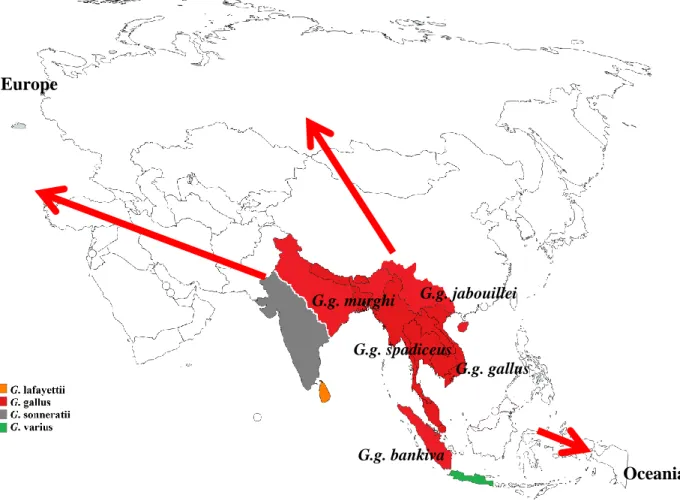
Chickens are of the family of Phasianidae and the genus Gallus. Four types or species of wild chickens are reported in the modern studies of birds, the red (Gallus gallus), grey (Gallus sonnerati), green (Gallus varius), and Ceylon (Gallus lafayettii) jungle fowls [1]. The origin of all these wild ancestors is distributed across South and Southeast Asia as well as Southwest China as demonstrated in Figure 1.1 [2]. The Gallus gallus presumably originates from South and Southeast Asia as well as from Southwest China (Yunnan province), the Gallus sonnerati from India, the Gallus varius from Java islands, and the Gallus lafayettii from Sri Lanka. The red jungle fowl (RJF) consists of five subspecies, G. gallus gallus, gallus spadiceus, gallus murghi, gallus bankiva and gallus jabouillei. Although it is not clear to what extent the other three wild type species contribute to the modern chickens, it has been established that the RJF is the main progenitor of the widely distributed chicken of today, the Gallus gallus domesticus [1–4]. Although it has been suggested that earliest domestication of chickens may have taken place around 6000 B.C. or earlier in China [2], research studies point out that the main precursor of widely spread today’s chicken diversity is from the domestication events that took place in the Indus Valley during 2500-2100 B.C.[1].
Figure 1.1: The distribution of chicken wild species. Red arrows show the westwards and eastwards directions of dispersion after domestication.
From centers of domestication in Asia to the world: a brief history of chicken dispersion The dispersion of chicken across the world has mainly been facilitated by human migration and trading. After domestication, chickens were taken westward to Europe and further eastwards to Island Southeast Asia and the Oceania/the Pacific [5]. Domesticated livestock including chickens mainly arrived in the Oceania regions when people colonized the islands [5, 6]. It is suggested that chickens were brought to the pacific islands in varying times which might date to as early as around 4500 B.P. [5].
G.g. murghi
G.g. bankiva
G.g. jabouillei
G.g. spadiceus
G.g. gallus Europe
Oceania
Europe. The main period of domestic chickens’ dispersion throughout Europe was around 450 to 1100 B.C. [2]. However, reports suggest that there has been chickens in Europe from as early as at least 4000 to 3000 B.C. [2, 4]. Chickens are believed to have been brought on two main routes into Europe, one through the south via Persia and Greece to the Mediterranean region and another one through the north via China and Russia to Northern Europe [1].
Africa. Information on dispersion of domestic chickens into Africa is very sketchy. Reports suggest that chickens existed in pictorial records in Egypt before 1400 B.C. [1]. The general belief is that chickens entered Africa from Asia through the Indian ocean coastline and from Europe through the north (Horn of Africa) [7, 8]. However, there is much speculations and lack of clarity on when exactly chickens reached the African continent and by which route or entry point. Studies based on analyzing mitochondrial DNA suggested that the most common and possibly the earliest haplogroup in Africa may be originating from South Asia (Indian subcontinent) and could have entered the eastern part of Africa through three possible routes: through the Middle East into Egypt, through the Horn of Africa or directly to Coastal East Africa [8].
The Americas. Chickens presumably arrived in the Americas quite late after the time of domestication and from several sources. Chickens were introduced to South America from Polynesia [9] and from Europe in the 15th century [10], additionally it is believed that Europeans also brought forth Asian breeds to South America as well as chickens from Africa through slave trading [5].
Main categories of breeds forming the global chicken diversity
From the wild species, many breeds and lines have been developed which are currently spread across the globe. While some breeds may have evolved naturally, many other breeds were also created by cross breeding and high selection programs to enhance or produce new phenotypes for different purposes. Below the main categories of chickens (local, fancy and commercial type breeds) are described. The classification is mainly based on the utilization of different breeding and management practices that have resulted in the current status of global chicken diversity.
Local breeds refer to the native and village or traditional chicken breeds, often indigenous, and well-adapted to the country or region. These breeds are usually raised in low input production systems [11]. In many developing countries, the chickens are kept under extensive production systems, they are usually kept in backyards, sleep on trees, house corners, scavenging for food or fed on left overs with limited or no supplementary food. There is also no/limited routine health check or vaccination against diseases, no structured breeding programs nor selection programs in place [12–14], and intercrossing occurs between nearby villages or populations [15–17]. In rural villages where many of these chickens are kept, the local chickens are mostly used for household consumption, to a less extent for sales, gifts and traditional rituals [12]. Local breeds are often associated with low productivity which poses challenges for their existence as local consumers become attracted to the productivity of commercial lines [14, 17].
Fancy breeds. Fancy breeding is characterized by breeding for physical appearance in accordance with the poultry standards e.g. [18, 19]. One of the oldest poultry standards were established by the British and got published in 1865 [19]. About a decade later, North America published their first standards for fancy breeding named the ‘American Standard of Perfection’ administered by the American Poultry Association (http://www.amerpoultryassn.com/). Many poultry breed
standards were established in the 19th century by poultry breeds’ associations and clubs in order to give complete description and guidelines of how a specific breed should look like. Therefore, participants aim to produce such an ideally ‘perfect’ description. The description could be for a particular physical appearance e.g. feather color, miniature, skin color, or for behavioral characteristics, e.g. fighters. In Europe, participants following the European Poultry Standards [18]
explored many phenotypes from breeds which have been maintained in Europe for decades and new breeds which were brought to Asia during the 19th century, either keeping them as purebreds or crossing them to produce new phenotypes. German fancy breeds present an important asset of genetic diversity which covers a wide variety of breeds. However, due to the strict requirements to meet these standards or the perfect phenotypes, breeders in these associations practice very refined selection for their breeding stock and even mate very closely related individuals in order to achieve the perfect phenotypes. Such practices may be detrimental as they enhance the loss of genetic diversity, propagate negative consequences of inbreeding and could endanger the survival of the breed.
Commercial breeds refer to breeds which are raised primarily for profit. Commercial chicken breeding companies are specialized in meat (broilers) and egg production types whereby breeds with good productive characteristics for either meat or eggs have been developed and subsequently selected for such traits. Currently, the commercial egg layers consist of two main types, the white and brown egg layers. The commercial chicken breeding industry now provides most chickens and is spread all over the world. Commercial breeding companies are characterized by sophisticated breeding programs including well defined breeding goals and highly intense production systems with strict health regime and elaborate housing and feed administration.
These three main types of breeds present a wide range of phenotypic features and make up the current global chicken diversity. The diversity ranges from different aspects of production, reproduction, growth and behavior (e.g., broodiness, fighters and recognition) as well as physical aspects (e.g., comb type and color, plumage color, shank length, egg thickness and color) [20–22].
Furthermore, there are differences at the genomic level which are underlying these phenotypic differences. The conservation of genetic variation is important for the preservation of the species especially in view of the increasingly alarming changes on the planet earth, e.g. global warming.
Genetic diversity studies are crucial to understand important genetic variants for different situations and conditions to effectively manage the chicken genetic resources as well as making informed decisions for current utilization and preservation of important genetic resources for the future [23].
Acquisition and use of genomic data for genetic diversity studies
Many studies have commonly used genetic markers especially microsatellites in chicken genetic diversity studies e.g. [7, 24]. Currently, the most popular types of genomic data used are the whole genome sequencing (WGS) and single nucleotide polymorphism (SNP) genotype data. Besides the WGS data, the SNP data is preferred among other genetic marker data because they are the most abundant form of genomic variation containing more in-depth information. Although the whole genome sequencing data is still the most effective way of studying the genome wide diversity, acquiring such data remains very expensive and requires additional infrastructure (e.g.
good reference genomes) and therefore poses more limitations to conduct large studies. Therefore, SNP genotyping is commonly used as an affordable alternative with less infrastructural requirement, less effort and time. SNP genotyping data is acquired by using already developed SNP panels such as genotyping arrays or chips. The single nucleotide polymorphisms in the panels
are acquired by sequencing a set of individuals which are selected from a limited number of populations. Specified criteria (e.g., minimum allele frequency, even distribution of SNPs across the genome) are then applied to select the SNP panel to be used. The selected SNP panels are used for the genotyping of many individuals from different populations. Because of the selection procedure of the SNPs, the SNP panels may suffer from ascertainment bias. Ascertainment bias is a systematic deviation in statistical population genetic measures from true values due biased marker discovery protocols [25].
Some of the problems or shortfalls that come with these methods of SNP discovery include the fact that since the discovery of SNPs is dependent on the allele frequency, there is less chance of discovering rare SNPs in a small sample set compared to the common SNPs and therefore, many rare SNPs are missing [26]. Consequently, the estimates of genetic diversity that depend on the allele frequencies will also be affected [27]. There may be overestimation of genetic diversity in some populations, especially in those that are included in the discovery panel [28]. Overall the classical population genetics methods are designed for whole genome data or randomly sampled SNPs across many loci and do not account for the ascertained genotype data. Therefore, when these methods are applied to SNP genotypes without accounting for ascertainment bias, they will produce inaccurate results [27, 29].
The high density SNP genotyping array for chicken
The latest and highest density array for the chicken was released in 2003, the 600K Affymetrix® Axiom® HD genotyping array for chicken [30]. The array was designed using twenty-four chicken lines, which consisted of fifteen commercial lines (4 broilers, 6 white egg layers and 5 brown layers), eight experimental inbred layer lines and one unselected layer line. It contains 580,954 SNPs of which 21,534 are coding variants, providing the opportunity to explore the genetic
diversity of chickens [30]. The work presented in chapters 2 to 4 is based on chicken data genotyped with the Affymetrix 600K genotyping array.
SNP annotation and functional classification
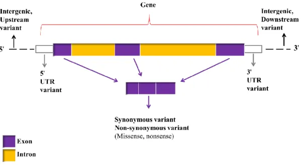
The first draft of the chicken reference genome, based on the red jungle fowl (Gallus gallus), was released in 2004 [31]. The development of the Affymetrix 600K genotyping array was based on the fourth version of the reference genome, the Gallus_gallus-4.0, which was released in 2011 containing 28 of the 38 autosomes, both sex chromosomes and two linkage groups. Currently, on the Affymetrix official webpage (now acquired by Thermo Fisher Scientific, https://www.thermofisher.com/de/de/home.html), the Affymetrix 600K genotyping array is accompanied by the annotation map based on the fifth version of the genome assembly, the Gallus_gallus-5.0 which contains three additional autosomes (GGA30, 31, and 33) [32]. However, a new version of the reference genome (Gallus_gallus-6.0) is already available. The Affymetrix Gallus_gallus-5.0 annotation map contains information of genes associated with the SNPs as well as the type of consequences of the SNPs. The SNP consequences were classified following the Ensembl variant predictor [33]. SNPs can be classified into two major groups, genic and intergenic (non-genic). Figure 1.2 shows the different SNP variants within and between the genes (for descriptions of SNP variants see Table 1.1).
Figure 1.2: Diagram showing the location of different SNP variants (modified from McLaren et al. 2010)
Table 1.1: Description of SNP variants Type of SNPs Description
Exonic SNPs Variants within the coding region of the gene, may or may not result in the alteration of the amino acids as follows:
the synonymous type refers to the sequence variant that does not change the amino acid,
the non-synonymous nucleotide substitution changes one or more
bases, resulting in a different amino acid sequence.
Intronic SNPs Variants within the noncoding region of a gene (introns) which is not translated into the protein.
5' UTR SNPs The transcribed SNPs located at the 5' end of the gene but are not translated into the protein.
3' UTR SNPs The transcribed SNPs located at the 3' end of the gene but are not translated into the protein.
Upstream SNPs Variants which are located adjacent to the 5' UTR region.
Downstream SNPs Variants which are located adjacent to the 3' UTR region.
Intergenic SNPs SNPs which are not part of the gene but are located in the upstream or downstream region.
Model for the cause of genetic differentiation between populations
The theory of ‘isolation by distance’ can be used to easily understand the cause of genetic differentiation between populations. The theory of ‘isolation by distance’ refers to the decrease in genetic relatedness with the increase in geographic distance [34, 35]. The theory was first introduced by Sewall Wright to articulate the patterns of differentiation under dispersal [35]. In a large, random mating population genetic differentiation may be brought forth by local patterns of selection or random mutations, as well as limited possibility of mating between those individuals that are not in close proximity. Such differentiation may result in the creation of certain population structures. However, the differentiation is limited to some extent by lack of isolation [36]. Ishida [37] describes Wright’s concept as ‘ecological isolation by distance’ as it concerns the local interaction of individuals. However, where genetic associations are restricted by geographic separations due to population migration, population genetic patterns reflect the differentiation among the subpopulations. This is termed the theory of ‘genetic isolation by distance’ according to Malécot [34]. Such differentiation under long geographic distances occurs because the consequences of genetic drift act more rapidly than the potential or chance of an individuals’
interaction under dispersal [38]. Therefore, in general, genetic relatedness of individuals is defined by the local (ecological) aspects and large distances of geographic separations.
A single founder migration model of genetic diversity
When a small number of individuals migrate from a single large population to form a new population in a new territory, they carry only a subset of the genetic diversity of that present in the large population. This phenomenon of the change in genetic diversity is called the ‘founder effect’
[39]. The smaller the migrated population, the more vulnerable it is to the effects of genetic drift, e.g. population bottlenecks. Not only does the migrated population lose genetic diversity due to
genetic drift, but it may also result in population differentiation from the founder population as described by the theory of ‘genetic isolation by distance’. If there is/are subsequent migration/s from the newly formed populations to farer distances, the genetic diversity further decreases, an event termed ‘serial founder effect’. Furthermore, genetic differentiation further increases between the subsequent migrants and the original founder population. Using the so called ‘Out of Africa’
theory, which assigns Africa as the origin of modern humans, studies have applied population genetics methods to establish the expansion of populations from a single founder as the best explanatory factor of the geographical patterns of genetic diversity within a species [40].
Measures of genetic diversity and population structure
There are many measures of genetic diversity between and within populations and in the following parts we briefly introduce some of those which have been often applied in this thesis.
Reynolds’ genetic distance
Reynolds’ genetic distance is a measure of population divergence by genetic drift [41]. This measure of distance is based on the coancestry coefficient and it is estimated as:
𝐷𝑅 = 1
2∑∑ (𝑝𝑖 1𝑖− 𝑝2𝑖)2 1 − ∑ (𝑝𝑖 1𝑖𝑝2𝑖)
𝑖
where 𝑖 is the 𝑖𝑡ℎ allele at bi-allelic loci and 𝑝1𝑖 is the frequency of the 𝑖𝑡ℎ allele at bi-allelic loci locus in population 1.
Heterozygosity
Heterozygosity is the state of having two different alleles at one locus. It is used as a measure of genetic variability within a population. The expected heterozygosity is calculated as:
𝐻𝑒 = 2𝑝 (1 − 𝑝)
where 𝑝 represents the allele frequency of one allele [42]. High fixation of alleles (e.g. by selection) results in the decrease in heterozygosity and therefore loss of genetic variability.
Wright’s fixation index (𝑭𝑺𝑻)
Wright’s fixation index is a popular measure of population differentiation and was introduced by Wright [43]. It measures the proportion of genetic variance between populations based on the allele frequencies with values ranging from 0 to 1, where 0 indicates that there is no genetic differentiation between populations. It is calculated as
𝐹𝑆𝑇 =𝜎𝑆2
𝜎𝑇2 = 𝜎𝑆2 𝑝̅ (1 − 𝑝̅)
where 𝜎𝑆2 is the variance of allele frequency between subpopulations and 𝜎𝑇2 is the variance of allele frequency in the total populations. In the ‘Methods’ section of chapter 2 we show how different sample sizes are accounted for following the recommendations of Weir and Cockerham [44].
Principal component analysis (PCA)
Principal component analysis is a statistical technique that transforms a high number of observed variables which are possibly correlated into low dimensional data of artificial, uncorrelated variables. These key variables, called principal components, account for most of the variation of the observations [45–47].PCA makes it easy to explore data and to visualize the relatedness of individuals or populations in a simpler form.
The aim and objectives
Studying and understanding the diversity of a species is crucial for making informed decisions for the conservation and effective management of farm animal genetic resources, as well as for understanding different evolutionary dynamics of the species. The main aim of the thesis was to investigate the genetic diversity in global chicken populations starting from the centers of chicken domestication in Asia. We had access to high density SNP genotype data and WGS data. The studies of genetic diversity based on SNP genotype data may produce misleading results due to ascertainment bias. Therefore, our first objective was to investigate different strategies to mitigate the effects of ascertainment bias when using SNP genotype data. The second objective was to investigate the overall genetic diversity between and within the globally collected chicken populations. The third objective was to investigate to what extent the observed overall genetic diversity in the chicken populations is a result of their genetic expansion from their wild founders in Asia.
References
[1] Crawford RD. Origin and history of poultry species. In: Crawford RD, editor. Poultry Breeding and Genetics. Amsterdam-Oxford-Newyork-Tokyo: Elsevier; 1990. p. 1–42.
[2] West B, Zhou BX. Did chickens go North? New evidence for domestication. J Archaeol Sci.
1988; 15: 515–33.
[3] Liu YP, Wu GS, Yao YG, Miao YW, Luikart G, Baig M, et al. Multiple maternal origins of chickens: Out of the Asian jungles. Mol Phylogenet Evol. 2006; 38: 12–9.
[4] Tixier-Boichard M, Bed’Hom B, Rognon X. Chicken domestication: From archeology to genomics. C R Biol. 2011; 334: 197–204.
[5] Storey AA, Athens JS, Bryant D, Carson M, Emery K, DeFrance S, et al. Investigating the global dispersal of chickens in prehistory using ancient mitochondrial dna signatures. PLoS One.
[2012; 7: e39171.
[6] Storey AA, Spriggs M, Bedford S, Hawkins SC, Robins JH, Huynen L, et al. Mitochondrial DNA from 3000-year old chickens at the Teouma Site , Vanuatu. J Archaeol Sci. 2010; 37: 2459–
68.
[7] Lyimo CM, Weigend A, Msoffe PL, Eding H, Simianer H, Weigend S. Global diversity and genetic contributions of chicken populations from African, Asian and European regions. Anim Genet. 2014; 45: 836–48.
[8] Mwacharo JM, Bjørnstad G, Mobegi V, Nomura K, Hanada H, Amano T, et al. Mitochondrial DNA reveals multiple introductions of domestic chicken in East Africa. Mol Phylogenet Evol.
2011; 58: 374–82.
[9] Storey AA, Ramírez JM, Quiroz D, Burley D V, Addison DJ, Walter R, et al. Radiocarbon and DNA evidence for a pre- Columbian introduction of Polynesian chickens to Chile Radiocarbon and DNA evidence for a pre-Columbian introduction of Polynesian chickens to Chile. Proc Natl Acad Sci. 2007; 104: 10335–10339.
[10] Gongora J, Rawlence NJ, Mobegi VA, Jianlin H, Alcalde JA, Matus JT, et al. Indo-European and Asian origins for Chilean and Pacific chickens revealed by mtDNA. Proc Natl Acad Sci. 2008;
105: 10308–13.
[11] Besbes B, Tixier-Boichard M, Hoffmann I, Jain G. Future trends for poultry genetic resources.
In: Proceedings of the International Conference of Poultry in the 21st Century: Avian Influenza
and Beyond. Bangkok; 2007.
[12] Ekue FN, Poné KD, Mafeni MJ, Nfi AN, Njoya J. Survey of the traditional poultry production system in the Bemenda area, Cameroon. FAO. 2002; January 2002: 15–25.
[13] Fathi M, El-Zarei M, Al-Homidan I, Abou-Emera O. Genetic diversity of Saudi native chicken breeds segregating for naked neck and frizzle genes using microsatellite markers. Asian- Australasian J Anim Sci. 2018; 31: 1871–80.
[14] Fulton JE, Berres ME, Kantanen J, Honkatukia M. MHC-B variability within the Finnish Landrace chicken conservation program. Poult Sci. 2017; 96: 3026–30.
[15] Adebambo AO, Mobegi VA, Mwacharo JM, Oladejo BM, Adewale RA, Iloro LO, et al. Lack of Phylogeographic Structure in Nigerian Village Chickens Revealed by Mitochondrial DNA D- loop Sequence Analysis Lack of Phylogeographic Structure in Nigerian Village Chickens Revealed by Mitochondrial DNA D-loop Sequence Analysis. Int J Poult Sci. 2010; 9: 503–7.
[16] Muchadeyi FC, Eding H, Wollny CBA, Groeneveld E, Makuza SM, Shamseldin R. Absence of population substructuring in Zimbabwe chicken ecotypes inferred using microsatellite analysis.
Anim Genet. 2007; 38: 332–9.
[17] Qu L, Li X, Xu G, Chen K, Yang H, Zhang L, et al. Evaluation of genetic diversity in Chinese indigenous chicken breeds using microsatellite markers. Sci China, Ser C Life Sci. 2006; 49: 332–
41.
[18] Rassegeflügel-Standard für Europa in Farbe. Bund Deutscher Rassegeflügelzüchter (ed.), Howa Druck & Satz GmbH, Fürth. ISBN 987–3–9806597-1-0.
[19] Tegetmeier WB. The Standard of Excellence in Exhibition Poultry, authorized by the Poultry Club. London: Groombridge and Sons; 1865.
[20] Dahloum L, Moula N, Halbouche M, Mignon-Grasteau S. Phenotypic characterization of the indigenous chickens (Gallus gallus) in the Northwest of Algeria. Arch Anim Breed. 2016; 59: 79–
90.
[21] Faruque S, Siddiquee N, Afroz M, Islam M. Phenotypic characterization of Native Chicken reared under intensive management system. J Bangladesh Agric Univ. 2010; 8: 79–82.
[22] Fathi MM, Al-homidan IH. Characterisation of Saudi native chicken breeds: a case study of morphological and productive traits. Worlds Poult Sci J. 2017; 73: 916–27.
[23] Tixier-Boichard M, Leenstra F, Flock DK, Hocking PM, Weigend S. A century of poultry genetics. Worlds Poult Sci J. 2012; 68: 307–21.
[24] Hillel J, Groenen MAM, Tixier-Boichard M, Korol AB, David L, Kirzhner VM, et al.
Biodiversity of 52 chicken populations assessed by microsatellite typing of DNA pools. Genet Sel Evol. 2003; 35: 533–57.
[25] Heslot N, Rutkoski J, Poland J, Jannink J-L, Sorrells ME. Impact of Marker Ascertainment Bias on Genomic Selection Accuracy and Estimates of Genetic Diversity. PLoS One. 2013; 8:
e74612.
[26] Clark AG, Hubisz MJ, Bustamante CD, Williamson SH. Ascertainment bias in studies of human genome-wide polymorphism. Genome Res. 2005; 15: 1496–502.
[27] Lachance J, Tishkoff SA. SNP ascertainment bias in population genetic analyses: Why it is
important, and how to correct it. BioEssays. 2013; 35: 780–6.
[28] Herrero-Medrano JM, Megens H-J, Groenen MA, Bosse M, Pérez-Enciso M, Crooijmans RP.
Whole-genome sequence analysis reveals differences in population management and selection of European low-input pig breeds. BMC Genomics. 2014; 15: 601.
[29] Nielsen R. Population genetic analysis of ascertained SNP data. Hum Genomics. 2004; 1:
218–24.
[30] Kranis A, Gheyas AA, Boschiero C, Turner F, Yu L, Smith S, et al. Development of a high density 600K SNP genotyping array for chicken. BMC Genomics. 2013; 14: 59.
[31] International Chicken Genome Sequencing Consortium. Sequence and comparative analysis of the chicken genome provide unique perspectives on vertebrate evolution. Nature. 2004; 432:
695–716.
[32] Warren WC, Hillier LW, Tomlinson C, Minx P, Kremitzki M, Graves T, et al. A New Chicken Genome Assembly Provides Insight into Avian Genome Structure. G3: Genes, Genomes, Genetics. 2017; 7: 109–17.
[33] McLaren W, Pritchard B, Rios D, Chen Y, Flicek P, Cunningham F. Deriving the consequences of genomic variants with the Ensembl API and SNP Effect Predictor.
Bioinformatics. 2010; 26: 2069–70.
[34] Malécot G. The mathematics of heredity. Translated by Yermanos DM. San Francisco, CA USA: Freeman; 1969.
[35] Wright S. Isolation by Distance. Genetics. 1943; 28: 114–38.
[36] Kimura M, Weiss GH. The Stepping Stone Model of Population Structure and the Decrease of Genetic Correlation with Distance. Genetics. 1964; 49: 561–76.
[37] Ishida Y. Sewall Wright and Gustave Malécot on Isolation by Distance. Philos Sci. 2009; 76:
784–96.
[38] Aguillon SM, Fitzpatrick JW, Bowman R, Schoech SJ, Clark AG, Coop G, et al.
Deconstructing isolation-by-distance: The genomic consequences of limited dispersal. PLoS Genet. 2017; 13: e1006911.
[39] Provine WB. Ernst Mayr: Genetics and speciation. Genetics. 2004; 167: 1041–6.
[40] Prugnolle F, Manica A, Balloux F. Geography predicts neutral genetic diversity of human populations. Curr Biol. 2005; 15: 159–60.
[41] Reynolds J, Weir BS, Cockerham CC. Estimation o f the coancestry coefficient: Basis for a short-term genetic distance. Genetics. 1983; 105: 767–79.
[42] Falconer DS, Mackay TFC. Introduction to Quantitative Genetics. 4th edition. Essex, UK:
Longmans Green, Harlow; 1996.
[43] Wright S. The Genetical Structure of Populations. Ann Eugen. 1951; 15: 322–54.
[44] Weir BS, Cockerham CC. Estimating F-Statistics for the Analysis of Population Structure.
Evolution. 1984; 38: 1358–70.
[45] Raychaudhuri S, Stuart JM, Altman RB. Principal Components Analysis to Summarize Microarray Experiments: Application to Sporulation Time Series. In: Pacific Symposium on Biocomputing. 2000. p. 455–66.
[46] Ringnér M. What is principal component analysis? Nat Biotechnol. 2008;26:303–4.
[47] Malomane DK, Norris D, Banga CB, Ngambi JW. Use of factor scores for predicting body weight from linear body measurements in three South African indigenous chicken breeds. 2014;
46: 331-335.
CHAPTER 2
Efficiency of different strategies to mitigate ascertainment bias when using SNP panels in diversity studies
Dorcus Kholofelo Malomane1,2, Christian Reimer1,2, Steffen Weigend2,3, Annett Weigend3, Ahmad Reza Sharifi1,2, Henner Simianer1,2
1Animal Breeding and Genetics Group, Department of Animal Sciences, University of Goettingen, Goettingen, Germany
2Center for Integrated Breeding Research, Department of Animal Sciences, University of Goettingen, Goettingen, Germany
3Institute of Farm Animal Genetics, Friedrich-Loeffler-Institut, Neustadt, Germany
Published in BMC Genomics
https://bmcgenomics.biomedcentral.com/articles/10.1186/s12864-017-4416-9
Abstract
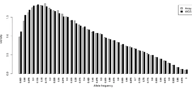
Background: Single nucleotide polymorphism (SNP) panels have been widely used to study genomic variations within and between populations. Methods of SNP discovery have been a matter of debate for their potential of introducing ascertainment bias, and genetic diversity results obtained from the SNP genotype data can be misleading. We used a total of 42 chicken populations where both individual genotyped array data and pool whole genome resequencing (WGS) data were available. We compared allele frequency distributions and genetic diversity measures (expected heterozygosity (𝐻𝑒), fixation index (𝐹𝑆𝑇) values, genetic distances and principal components analysis (PCA)) between the two data types. With the array data, we applied different filtering options (SNPs polymorphic in samples of two Gallus gallus wild populations, linkage disequilibrium (LD) based pruning and minor allele frequency (MAF) filtering, and combinations thereof) to assess their potential to mitigate the ascertainment bias.
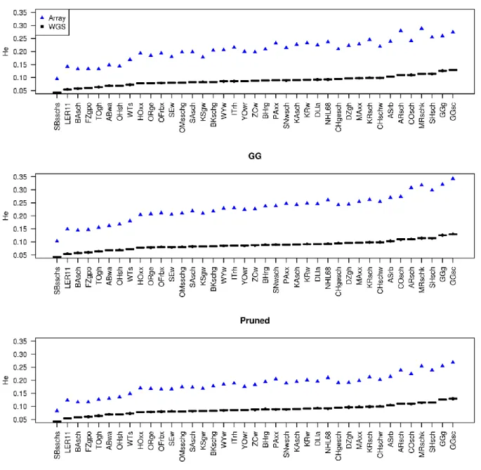
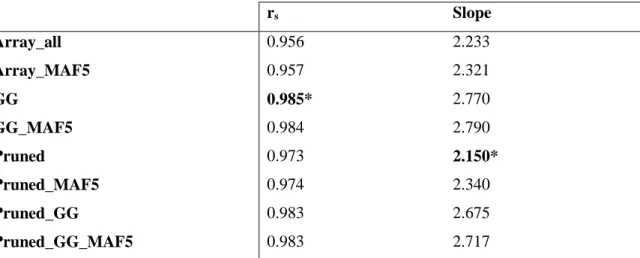
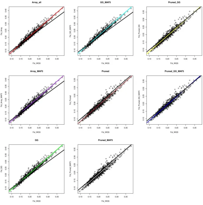
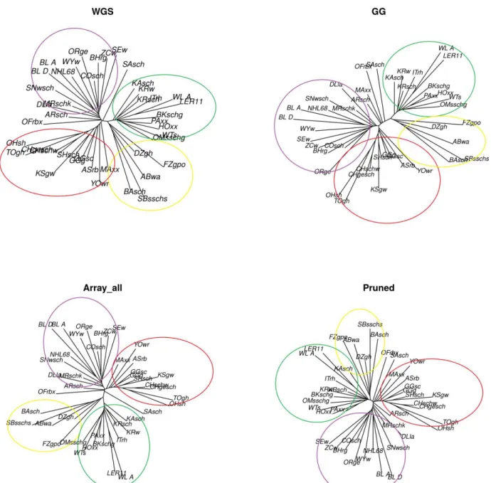
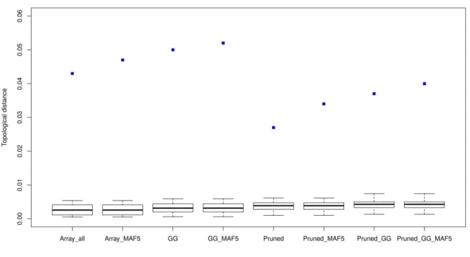
Results: Rare SNPs were underrepresented in the array data. Array data consistently overestimated 𝐻𝑒 compared to WGS data, however, with a similar ranking of the breeds, as demonstrated by Spearman’s rank correlations ranging between 0.956 and 0.985. LD based pruning resulted in a reduced overestimation of 𝐻𝑒 compared to the other filters and slightly improved the relationship with the WGS results. The raw array data and those with polymorphic SNPs in the wild samples underestimated pairwise 𝐹𝑆𝑇 values between breeds which had low 𝐹𝑆𝑇 (<0.15) in the WGS, and overestimated this parameter for high WGS 𝐹𝑆𝑇 (>0.15). LD based pruned data underestimated 𝐹𝑆𝑇 in a consistent manner. The genetic distance matrix from LD pruned data was more closely related to that of WGS than the other array versions. PCA was rather robust in all array versions, since the population structure on the PCA plot was generally well captured in comparison to the WGS data.
Conclusions: Among the tested filtering strategies, LD based pruning was found to account for the effects of ascertainment bias in the relatively best way, producing results which are most comparable to those obtained from WGS data and therefore is recommended for practical use.
Background
Following the process of animal domestication, evolutionary forces such as selection and genetic drift have played a critical role in animal diversification. Such forces led to genomic alterations such as fixation of favorable alleles within a breed or species and differentiation from the ancestral state due to successful selection programs or adaptation. This concept of domestication and its subsequent impact on diversity of animal species, breeds or strains was well explored by Darwin [1, 2]. So, phylogenetic studies aim to assess these variations.
The wild, unselected native and village chicken populations retain a reservoir of and exhibit more genetic variability [3–5]. Commercial breeds are known for being intensely selected for economic purposes, i.e. meat and egg type production. Successful egg type selection programs within the commercial layers have resulted in a reduced genetic variability within these lines. In Europe, an organized and systematic breeding in chickens was developed during the 19th century. Selection programs in this case were based on producing attractive features (for entertainment) in line with the breed standards; because of this, many fancy breeds were heavily selected for their attractiveness. To date such heavily selected breeds exhibit reduced genetic diversity and high average genetic distances to other breeds [3–5]. Major components for the reduced variability within both the commercial and the fancy breeds are due to the fact that the selection was certainly based on small number of founders, small effective population size and/or high degree of inbreeding.
Using whole genome resequencing (WGS) data is considered as the best way of doing association or diversity studies [6, 7]. It provides a high resolution of the genome information capturing most (and even the finer) details underlying genomic variations. However, the cost of whole genome sequencing still is high for application in larger sample sets. Additionally, limitations such as infrastructure (e.g. WGS requires good reference genomes), work effort and time poses further constraints. So, generating WGS data for the required sample size in such studies is challenging [6].
Genotyping tools have been developed to overcome these constraints and have made genotype data available in sufficient numbers. Single nucleotide polymorphism (SNP) panels have been widely used in studies of genomic variation within species [8, 9]. For the construction of such SNP sets, a limited number of individuals selected from populations of interest (the so-called ascertainment group) are used as discovery panels. These individuals are sequenced and provide the basis to select polymorphic loci targeted for further genotyping in a larger set of individuals [9, 10]. SNPs are often selected based on quality, with predefined spacing (e.g. equally spaced) and desired frequency distribution [10], among other criteria.
These methods of SNP discovery may introduce ascertainment bias, hindering classical population genetic methods to provide correct results when applied with SNP genotype data [11, 12].
Ascertainment bias is a systematic deviation of population genetic statistics from a theoretical
‘true’ value, which arises from a non-random selection of set of individuals or biased marker discovery protocols [6, 13].
If the level of ascertainment bias is high, results of population genetic studies could be widely misinterpreted [14]. Thus, exploring the potential systematic effects that the ascertained genotype
data can have on the results of diversity studies and finding a way to minimize these effects is crucial.
Differences in the allele frequency distribution between SNP genotype data and WGS data have been commonly used to assess ascertainment bias [6, 11, 15]. An easily verifiable indicator of a potential ascertainment bias is a complete absence of SNPs or an underrepresentation of rare SNPs.
Discovery of SNPs is driven by the allele frequency, and with an often small size of the discovery panel, discovering rare SNPs is mostly limited [14]. With the missing rare SNPs, the SNP data may not be an adequate representation of the WGS data. Gorlov et al. [16] argue that missing rare SNPs can lead to loss of valuable information and lessen the ability to detect those rare SNPs in association studies, which may be critical e.g. in the context of rare causal SNPs for rare diseases.
Effects of ascertainment bias on genetic diversity analysis within and between populations have been reported in several studies [9, 13, 17]. One of the assertions is that selection of subpopulations for discovery panels tends to over-represent variability of that ascertainment group. Consequently, effects of ascertainment bias on heterozygosity estimates [18, 19], fixation index (𝐹𝑆𝑇) values and phylogenetic relationships [9] have been reported. Herrero-Medrano et al. [18] and Albrechtsen et al. [15] observed that ascertainment bias affected some populations more than others when studying their genetic diversity with SNP chip data. McTavish & Hillis [9] concluded that both the 𝐹𝑆𝑇 and principal components analysis (PCA) estimated from SNP chip data were distorted when ascertainment bias was not accounted for. Principal components analysis is a statistical technique that captures patterns of high dimensional data and projects them into a lower dimensional space, allowing to determine key variables that explain the observations [20, 21]. PCA has been used in many studies to capture genetic structures of populations [22–26]. In contrary to McTavish &
Hillis [9], McVean [27] reported that the PCA is less affected by ascertainment bias. He claims
that effects of ascertainment bias on PCA are easy to predict and only have little impact on the structuring of populations unless the bias is very severe.
Despite the available proposed schemes and several suggestions made on how to address the issue of ascertainment bias in population genetic analysis [6, 12, 15], there are still challenges on the definite measures to deal with this issue [17]. Clark et al. [14] concluded that it is not always easy to correct for ascertainment bias, success is not guaranteed, and mostly the suggested corrections are not applicable to every study [15]. Most of the suggestions were also tested using simulated data, which may miss out some of the complexities encountered when using real data.
In this study, we tried to assess the impact of ascertainment bias and the efficiency of various strategies to account for it in a chicken diversity panel, which is based on a diverse set of chicken populations for which both pooled WGS data and individual SNP genotype data obtained with a high density SNP array were available.For most of the studied populations, there is no sufficient documentation on the breed history and/or background and we are skeptic that the material used allows to identify the mechanisms causing ascertainment bias. Therefore, we based our primary focus on identifying strategies to mitigate ascertainment bias rather than to do a full analytical (or empirical) study to understand the causes of ascertainment bias. With the SNP genotyping array [10] that was used, the SNP panel was established by selecting a few populations (for details please see the “Methods” section) which are not representative for all the other populations used in our study. In addition, the SNP selection criterion included discarding low minor allele frequency (MAF) SNPs which potentially causes an underrepresentation of SNPs under selection [28].
Criteria used in our study to assess the impact of ascertainment bias and the various strategies to mitigate its effects were similarity of allele frequency spectra, expected heterozygosity, 𝐹𝑆𝑇, PCA, distance measures and topologies of phylogenetic trees. In general, the results obtained from the
WGS data were considered as the ‘reference standard’ and strategies to correct for ascertainment bias were considered based on how good the WGS-based results were met.
Methods Animals
A total of 42 chicken populations were used in this study. For each of the populations, both whole genome resequencing data based on pooled samples and individual genotype data obtained with a 600K SNP Affymetrix® Axiom® High Density Chicken Genotyping Array were available. A list of the 42 populations with their abbreviations and population sizes as used in the study is provided in Table 2.1. Samples used in this study were collected under the umbrella of the SYNBREED project (www.synbreed.tum.de) from chicken fancy breeds in Germany between 2010 and 2012.
The collection was completed by samples of two Red Jungle fowl populations, Gallus gallus gallus (GGg) and Gallus gallus spadiceus (GGsc) taken from previous EU project AVIANDIV (see [29]).
For the WGS pooled data, equal amounts of DNA of the individuals of each population were pooled using PicoGreen® quantitation assay except for the WL_A. In the case of WL_A, 10 birds were sequenced individually and virtual pooling was performed. Thirty-nine of the 42 populations in the WGS consisted of 385 individuals of which 383 were also genotyped individually. The other 3 populations (WL_A, BL_A and BL_D) were commercial lines (see Table 2.1) and consisted of different individuals in the two data sets. In the array data set, in addition to the 383 individuals, 461 more individuals were added and their distribution is also shown in Table 2.1. So, when comparisons were made between array and WGS data with commercial breeds included, the 383 plus 461 individuals’ version of array data was used. For the commercial breeds, each breed contained 20 individuals in the array data. In the WGS data, each breed contained 9-10 individuals
for the non-commercials and 10-15 individuals for the commercial breeds. The commercial breeds were among the breeds used in the discovery panel for the development of the 600K Affymetrix genotyping array.
Collection of blood samples for this study was performed in accordance with the German Animal Protection Law and was submitted to and approved by the Committee of Animal Welfare at the Institute of Farm Animal Genetics (Friedrich-Loeffler-Institut) and the Lower Saxony State Office for Consumer Protection and Food Safety (No. 33.9-42502-05-10A064).
Table 2.1: List of breeds, their abbreviations and sample sizes as used in the study Breed and abbreviation Array data (n) WGS data (n) Commercial breeds :
WL_A – White Leghorn line A 20* 10*
BL_A – Rhode Island Red line A 20* 15*
BL_D – White Rock line D 20* 15*
Wild populations :
GGg – Gallus Gallus Gallus 10(10) 10
GGsc – Gallus Gallus Spadiceus 9(10) 9
European populations:
ABwa – Barbue d’Anvers quail 10(10) 10
ARsch – Rumpless Araucana black 9(11) 9
BAsch – Rosecomb Bantam black 10(10) 10
BKschg – Bergische Crower 10(22) 10
DZgh – German Bantam gold partridge 10(10) 10
FZgpo – Booted Bantam millefleur 10(10) 10
HOxx – Dutch White Crested 10(7) 10
ITrh – Leghorn brown 10(10) 10
KAsch – Castilians black 9(11) 9
KRsch – Creeper black 10(20) 10
KRw – Creeper white 10(20) 10
LER11- White Leghorn line R11 9(13) 9(1)
OMsschg - East Friesian Gulls silver penciled 10(10) 10
PAxx - Poland any colour 11(12) 11
SBsschs - Sebright Bantam silver 10(10) 10
WTs - Westphalian Chicken silver 10(10) 10
Asian populations:
ASrb – Aseel red mottled 10(10) 10
BHrg – Brahma gold 10(10) 10
CHgesch – Japanese Bantam black tailed buff 10(12) 10 CHschw – Japanese Bantam black mottled 10(19) 10
COsch – Cochin black 10(11) 10
DLIa – German Faverolles salmon 10(10) 10
KSgw – Ko Shamo black-red 9(13) 9
MAxx – Malay black red 10(21) 10
MRschk – Marans copper black 10(10) 10
NHL68 – New Hampshire line 68 9(14) 9(1)
OFrbx – Orloff red spangled 10(15) 10
OHsh - Ohiki silver duckwing 10(10) 10
ORge - Orpington buff 10(10) 10
SAsch - Sumatra black 9(11) 9
SEw - Silkies white 10(10) 10
SHsch - Shamo black 9(11) 9
SNwsch - Sundheimer light 10(10) 10
TOgh - Toutenkou black breasted red 10(11) 10
WYw - Wyandotte white 10(9) 10
YOwr - Yokohama red saddled white 10(10) 10
ZCw - Pekin Bantam white 10(10) 10
n is number, in brackets () are additional individuals added to the population (not present in the other data type), *completely different individuals in the two data sets
WGS data and preparation
Pools of the 42 populations comprising in total 425 individuals were resequenced with 20X target coverage. The sequence reads were aligned to the chicken reference genome (galGal4) [30] using Burrows-wheeler alignment algorithm implemented in BWA [31] and sorted using Samtools [32].
Picard tools were used to mark duplicates and GATK was used for calling the SNPs [33, 34]. For more details on the preparation pipeline see Reimer et al. [35].
Genotype (array) data and filtering
The initial array data set contained 918 animals and 580, 588 SNPs. SNPs misplaced at wrong chromosomes were removed. The data was then filtered for SNP call rates of >99% and animal call rate of >95% using the SNP & Variation Suite Version (SVS) 8.1[36] which retained 904 animals and 450, 082 SNPs. From this point, the following SNP filtering pipeline was applied, with number of SNPs left at each step shown in brackets:
1. SNPs with missing positions were discarded (445,428).
2. SNPs that shared the same position on the same chromosome were discarded (e.g. if there were two SNPs sharing the same position, both of them were discarded (445,388).
3. SNPs had to be present in both array and WGS data (21,759 of array SNPs were not found in the WGS data) and only SNPs from chromosome 1-28 were considered (401,420).
4. SNPs were discarded if the reference (and/or alternative) allele of genotype (array) data didn’t match the reference (and/or alternative) allele from the sequence data (401,125).
After the above filtering, a total of 401,125 SNPs remained for further analysis. This set of data was used in assessing allele frequency calling in the pooled sequence data, comparing allele frequencies between the array and WGS data, and assessing how this uncorrected ascertained data
affect genetic diversity analysis by being compared to results analyzed from WGS. The array data SNP was converted so that allele A resembled the respective reference allele.
Different filtering schemes were applied to the array dataset (Array_all in Table 2.2) to be tested for their potential to account for ascertainment bias. More specifically, we applied three different basic filtering principles:
1. LD based SNP pruning, which has been described to partially account for the effects of ascertainment bias. In our study, SNP pruning for LD was done in PLINK v1.9 [37, 38]. The parameters: indep 50 5 2 were used, whereby 50 is the window size in SNPs, 5 is the window size step (in SNPs) after LD calculation (after LD has been calculated from the 50 SNPs window, and SNPs which exceed the VIF threshold are removed, the window is shifted 5 SNPs forward and the procedure is repeated), and 2 is the variance inflation factor VIF = 1/(1-r2) [39].
2. A second filter applied was to restrict the analysis to SNPs that were found to be polymorphic in the wild chicken populations, which were represented in our study with two populations (GGsc and GGg subspecies).
3. A third filter excluded SNPs with less than 5% MAF. This MAF filtering was done in PLINK v1.9 [37, 38] using the command –maf 0.05.
These filters were applied alone and in combination, the corresponding filters and resulting data sets are presented in Table 2.2.