Topics in Occupation Times and Gaussian Free Fields
Alain-Sol Sznitman
∗Notes of the course “Special topics in probability”
at ETH Zurich during the Spring term 2011
∗ Mathematik, ETH Z¨urich. CH-8092 Z¨urich, Switzerland
With the support of the grant ERC-2009-AdG 245728-RWPERCRI
I gave at ETH Zurich during the Spring term 2011. One of the objectives was to explore the links between occupation times, Gaussian free fields, Poisson gases of Markovian loops, and random interlacements. The stimulating atmosphere during the live lectures was an encouragement to write a fleshed-out version of the handwritten notes, which were handed out during the course. I am immensely grateful to Pierre-Fran¸cois Rodriguez, Art..em Sapozhnikov, Bal´azs R´ath, Alexander Drewitz, and David Belius, for their numerous comments on the successive versions of these notes.
Contents
0 Introduction 1
1 Generalities 5
1.1 The set-up . . . 5
1.2 The Markov chain X
.
(with jump rate 1) . . . 61.3 Some potential theory . . . 10
1.4 Feynman-Kac formula . . . 20
1.5 Local times . . . 22
1.6 The Markov chain X
.
(with variable jump rate) . . . 232 Isomorphism theorems 27 2.1 The Gaussian free field . . . 27
2.2 The measures Px,y . . . 30
2.3 Isomorphism theorems . . . 35
2.4 Generalized Ray-Knight theorems . . . 38
3 The Markovian loop 51 3.1 Rooted loops and the measure µr on rooted loops . . . 51
3.2 Pointed loops and the measure µp on pointed loops . . . 58
3.3 Restriction property . . . 61
3.4 Local times . . . 62
3.5 Unrooted loops and the measure µ∗ on unrooted loops . . . 67
4 Poisson gas of Markovian loops 71 4.1 Poisson point measures on unrooted loops . . . 71
4.2 Occupation field . . . 72
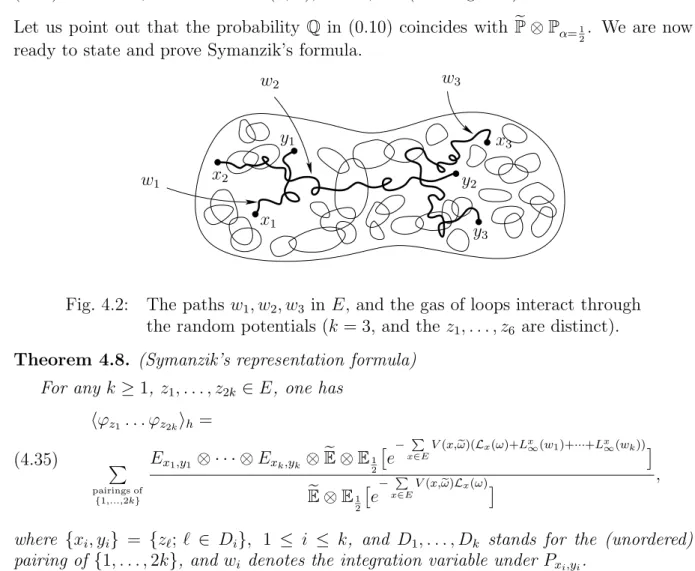
4.3 Symanzik’s representation formula . . . 76
4.4 Some identities . . . 80
4.5 Some links between Markovian loops and random interlacements . . . 84
References 93
Index 95
1
0 Introduction
This set of notes explores some of the links between occupation times and Gaussian pro- cesses. Notably they bring into play certain isomorphism theorems going back to Dynkin [4], [5] as well as certain Poisson point processes of Markovian loops, which originated in physics through the work of Symanzik [26]. More recently such Poisson gases of Marko- vian loops have reappeared in the context of the “Brownian loop soup” of Lawler and Werner [16] and are related to the so-called “random interlacements”, see Sznitman [27].
In particular they have been extensively investigated by Le Jan [17], [18].
A convenient set-up to develop this circle of ideas consists in the consideration of a finite connected graph E endowed with positive weights and a non-degenerate killing measure. One can then associate to these data a continuous-time Markov chainXt,t ≥0, onE, with variable jump rates, which dies after a finite time due to the killing measure, as well as
the Green densityg(x, y), x, y ∈E, (0.1)
(which is positive and symmetric), the local timesLxt =
Z t 0
1{Xs=x}ds, t≥0, x∈E.
(0.2)
In fact g(·,·) is a positive definite function on E ×E, and one can define a centered Gaussian processϕx, x∈E, such that
(0.3) cov(ϕx, ϕy)(= E[ϕxϕy]) =g(x, y), for x, y ∈E. This is the so-called Gaussian free field.
It turns out that 12ϕ2z,z ∈E, andLz∞,z ∈E, have intricate relationships. For instance Dynkin’s isomorphism theorem states in our context that for any x, y ∈E,
Lz∞+1
2ϕ2z
z∈E underPx,y⊗PG, (0.4)
has the “same law” as
1
2(ϕ2z)z∈E under ϕxϕyPG, (0.5)
where Px,y stands for the (non-normalized) h-transform of our basic Markov chain, with the choice h(·) =g(·, y), starting from the point x, and PG for the law of the Gaussian field ϕz,z ∈E.
Eisenbaum’s isomorphism theorem, which appeared in [7], does not involveh-transforms and states in our context that for any x∈E, s6= 0,
Lz∞+1
2(ϕz+s)2
z∈E under Px⊗PG, (0.6)
has the “same law” as
1
2(ϕz +s)2
z∈E under 1 + ϕx
s PG. (0.7)
The above isomorphism theorems are also closely linked to the topic of theorems of Ray- Knight type, see Eisenbaum [6], and chapters 2 and 8 of Marcus-Rosen [19]. Originally, see [13, 21], such theorems came as a description of the Markovian character in the space variable of Brownian local times evaluated at certain random times. More recently, the Gaussian aspects and the relation with the isomorphism theorems have gained promi- nence, see [8], and [19].
Interestingly, Dynkin’s isomorphism theorem has its roots in mathematical physics.
It grew out of the investigation by Dynkin in [4] of a probabilistic representation formula for the moments of certain random fields in terms of a Poissonian gas of loops interacting with Markovian paths, which appeared in Brydges-Fr¨ohlich-Spencer [2], and was based on the work of Symanzik [26].
The Poisson point gas of loops in question is a Poisson point process on the state space of loops onEmodulo time-shift. Its intensity measure is a multipleαµ∗ of the imageµ∗ of a certain measureµrooted, under the canonical map for the equivalence relation identifying rooted loopsγthat only differ by a time-shift. This measure µrooted is theσ-finite measure on rooted loops defined by
(0.8) µrooted(dγ) = P
x∈E
Z ∞ 0
Qtx,x(dγ) dt t ,
where Qtx,x is the image of 1{Xt = x}Px under (Xs)0≤s≤t, if X
.
stands for the Markov chain on E with jump rates equal to 1 attached to the weights and killing measure we have chosen on E.The random fields on E alluded to above, are motivated by models of Euclidean quantum field theory, see [11], and are for instance of the following kind:
(0.9) hF(ϕ)i= Z
RE
F(ϕ)e−12E(ϕ,ϕ)Q
x∈E
hϕ2x 2
dϕx
. Z
RE
e−12E(ϕ,ϕ)Q
x∈E
hϕ2x 2
dϕx
with
h(u) = Z ∞
0
e−vudν(v), u≥0, withν a probability distribution on R+,
andE(ϕ, ϕ) the energy of the functionϕcorresponding to the weights and killing measure onE (the matrixE(1x,1y),x, y ∈E is the inverse of the matrixg(x, y),x, y ∈E in (0.3)).
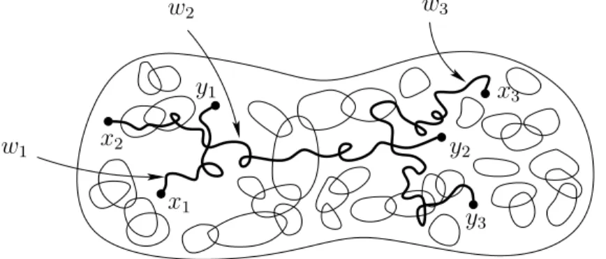
x2
x3
y1
w2 w3
w1 y2
x1
y3
Fig. 0.1: The paths w1, . . . , wk inE interact with the gas of loops through the random potentials.
3 The typical representation formula for the moments of the random field in (0.9) looks like this: for k≥1, z1, . . . , z2k ∈E,
(0.10)
hϕz1. . . ϕz2ki= P
pairings ofz1, . . . , z2k
Px1,y1 ⊗ · · · ⊗Pxk,yk ⊗Q[e−Px∈Evx(Lx+Lx∞(w1)+···+Lx∞(wk))] Q
e−Px∈EvxLx ,
where the sum runs over the (non-ordered) pairings (i.e. partitions) of the symbols z1, z2, . . . , z2k into {x1, y1}, . . . ,{xk, yk}. Under Q the vx, x ∈ E, are i.i.d. ν-distributed (random potentials), independent of the Lx, x ∈ E, which are distributed as the total occupation times (properly scaled to take account of the weights and killing measure) of the gas of loops with intensity 12µ, and the Pxi,yi, 1 ≤ i ≤ k are defined just as below (0.4), (0.5).
The Poisson point process of Markovian loops has many interesting properties. We will for instance see that whenα = 12 (i.e. the intensity measure equals 12µ),
(0.11) (Lx)x∈E has the same distribution as 12(ϕ2x)x∈E, where (ϕx)x∈E stands for the Gaussian free field in (0.3).
The Poisson gas of Markovian loops is also related to the model of random interlacements [27], which loosely speaking corresponds to “loops going through infinity”. It appears as well in the recent developments concerning conformally invariant scaling limits, see Lawler-Werner [16], Sheffield-Werner [24]. As for random interlacements, interestingly, in place of (0.11), they satisfy an isomorphism theorem in the spirit of the generalized second Ray-Knight theorem, see [28].
5
1 Generalities
In this chapter we describe the general framework we will use for the most part of these notes. We introduce finite weighted graphs with killing and the associated continuous- type Markov chainsX
.
, with constant jump rate equal to 1, and X.
, with variable jump rate. We also recall various notions related to Dirichlet forms and potential theory.1.1 The set-up
We introduce in this section the general set-up, which we will use in the sequel, and recall some classical facts. We also refer to [14] and [10], where the theory is developed in a more general framework. We assume that
(1.1) E is a finite non-empty set
endowed with non-negative weights
(1.2) cx,y =cy,x ≥0, forx, y ∈E, and cx,x= 0, for x∈E, so that
E, endowed with the edge set consisting of the pairs {x, y} such that (1.3)
cx,y >0, is a connected graph.
We also suppose that there is a killing measure onE:
(1.4) κx ≥0, x∈E,
and that
(1.5) κx6= 0, for at least some x∈E.
We also consider a
(1.6) cemetery state ∆ not in E
(we can think of κx as cx,∆).
With these data we can define a measure on E:
(1.7) λx = P
y∈E
cx,y+κx, x∈E (note that λx >0, due to (1.2) - (1.5)).
We can also introduce the energyof a function on E, or Dirichlet form (1.8) E(f, f) = 1
2
P
x,y∈E
cx,y(f(y)−f(x))2+ P
x∈E
κxf2(x), for f :E →R.
Note that (cx,y)x,y∈E and (κx)x∈E determine the Dirichlet form. Conversely, the Dirich- let form determines (cx,y)x,y∈E and (κx)x∈E. Indeed, one defines, by polarization, for f, g:E →R,
E(f, g) = 1
4[E(f+g, f+g)− E(f−g, f −g)]
= 1
2
P
x,y∈E
cx,y(f(y)−f(x))(g(y)−g(x)) + P
x∈E
κxf(x)g(x), (1.9)
and one notes that
E(1x,1y) =−cx,y, for x6=y in E, E(1x,1x) = P
y∈E
cx,y+κx =λx, for x∈E, (1.10)
so that the Dirichlet form uniquely determines the weights (cx,y)x,y∈E and the killing measure (κx)x∈E. Observe also that by (1.3), (1.5), (1.8), (1.9), the Dirichlet form defines a positive definite quadratic form on the spaceF of functions fromE toR, see also (1.39) below.
We denote by (·,·)λ the scalar product in L2(dλ):
(1.11) (f, g)λ = P
x∈E
f(x)g(x)λx, forf, g:E →R.
The weights and the killing measure induce a sub-Markovian transition probability on E:
(1.12) px,y = cx,y
λx
, for x, y ∈E, which is λ-reversible:
(1.13) λxpx,y =λypy,x, for all x, y ∈E.
One then extends px,y, x, y ∈E to a transition probability on E∪ {∆} by setting
(1.14) px,∆= κx
λx
, forx∈E, and p∆,∆= 1,
so the corresponding discrete-time Markov chain on E∪ {∆} is absorbed in the cemetery state ∆ once it reaches ∆. We denote by
(1.15)
Zn, n≥0, the canonical discrete Markov chain on the space of discrete trajectories in E∪ {∆}, which after finitely many steps reaches ∆ and from then on remains at ∆,
and by
(1.16) Px the law of the chain starting fromx∈E∪ {∆}.
We will attach to the Dirichlet form (1.8) (or, equivalently, to the weights and the killing measure), two continuous-time Markov chains onE∪ {∆}, which are time change of each other, with discrete skeleton corresponding to Zn, n ≥0. The first chain X
.
will have a unit jump rate, whereas the second chain X.
(defined in Section 1.6) will have a variable jump rate governed by λ.1.2 The Markov chain X. (with jump rate 1)
We introduce in this section the continuous-time Markov chain on E∪ {∆} (absorbed in the cemetery state ∆), with discrete skeleton described by Zn, n ≥ 0, and exponential
1.2 The Markov chain X
.
(with jump rate 1) 7 holding times of parameter 1. We also bring into play some of the natural objects attached to this Markov chains.The canonical space DE for this Markov chain consists of right-continuous functions with values in E ∪ {∆}, with finitely many jumps, which after some time enter ∆ and from then on remain equal to ∆. We denote by
Xt, t≥0, the canonical process on DE, (1.17)
θt, t≥ 0, the canonical shift onDE: θt(w)(·) =w(·+t), forw∈DE, Px the law on DE of the Markov chain starting at x∈E∪ {∆}.
Remark 1.1. Whenever convenient we will tacitly enlarge the canonical space DE and work with a probability space on which (under Px) we can simultaneously consider the discrete Markov chain Zn, n≥0, with starting point a.s. equal to x, and an independent sequence of positive variables Tn, n ≥ 1, the “jump times”, increasing to infinity, with increments Tn+1 −Tn, n ≥ 0, i.i.d. exponential with parameter 1 (with the convention T0 = 0). The continuous-time chain Xt, t≥0, will then be expressed as
Xt=Zn, for Tn≤t < Tn+1, n≥0.
Of course, once the discrete-time chain reaches the cemetery state ∆, the subsequent
“jump times” Tn are only fictitious “jumps” of the continuous time chain.
Examples:
1) Simple random walk on the discrete torus killed at a constant rate E = (Z/NZ)d, where N >1,d≥1,
endowed with the graph structure, where x, y are neighbors if exactly one of their coordinates differs by ±1, and the other coordinates are equal. We pick
cx,y = 1{x, y are neighbors}, x, y ∈E, κx =κ >0.
So Xt, t ≥ 0, is the simple random walk on (Z/NZ)d with exponential holding times of parameter 1, killed at each step with probability 2d+κκ , when N > 2, and probability d+κκ , when N = 2.
2) Simple random walk on Zd killed outside a finite connected subset of Zd, that is:
E is a finite connected subset of Zd, d≥1.
cx,y = 1{|x−y|=1}, for x, y ∈E, κx = P
y∈Zd\E
1{|x−y|=1}, forx∈E,
x′ E
x
κx′ = 0
κx = 2
Fig. 1.1
Xt, t ≥ 0, when starting in x ∈ E, corresponds to the simple random walk in Zd with exponential holding times of parameter 1 killed at the first time it exists E.
Our next step is to introduce some natural objects attached to the Markov chain X
.
, suchas the transition semi-group, and the Green function.
Transition semi-group and transition density:
Unless otherwise specified, we will tacitly view real-valued functions on E, as functions on E∪ {∆}, which vanish at the point ∆.
Thesub-Markovian transition semi-group of the chainXt,t≥0, on E is defined for t≥0, f :E →R, by
Rtf(x) =Ex[f(Xt)] for x∈E
= P
n≥0
e−t tn
n! Ex[f(Zn)]
= P
n≥0
e−t tn
n! Pnf(x) =et(P−I)f(x), (1.18)
where I denotes the identity map on RE, and for f: E →R,x∈E,
(1.19) P f(x) = P
y∈E
px,yf(y)(1.15)= Ex[f(Z1)].
As a result of (1.13) and (1.18)
P and Rt (for any t≥0) are bounded self-adjoint operators on L2(dλ), (1.20)
Rt+s =RtRs, for t, s≥0 (semi-group property).
(1.21)
We then introduce the transition density (1.22) rt(x, y) = (Rt1y)(x) 1
λy
, for t≥0, x, y ∈E.
It follows from the self-adjointness of Rt, cf. (1.20), that
(1.23) rt(x, y) =rt(y, x), for t≥0, x, y ∈E (symmetry)
1.2 The Markov chain X
.
(with jump rate 1) 9 and from the semi-group property, cf. (1.21), that for t, s≥ 0,x, y ∈E,(1.24) rt+s(x, y) = P
z∈E
rt(x, z)rs(z, y)λz (Chapman-Kolmogorov equations).
Moreover due to (1.3), (1.12), (1.18), we see that
(1.25) rt(x, y)>0, fort >0, x, y ∈E.
Green function:
We define the Green function (or Green density):
(1.26) g(x, y) = Z ∞
0
rt(x, y)dt(1.18),(1.22) Fubini= Ex
h Z ∞
0
1{Xt=y}dti 1 λy
, for x, y ∈E.
Lemma 1.2.
(1.27) g(x, y)∈(0,∞) is a symmetric function on E×E.
Proof. By (1.23), (1.25) we see that g(·,·) is positive and symmetric. We now prove that it is finite. By (1.1), (1.3), (1.5) we see that for some N ≥0, and ε >0,
(1.28) inf
x∈EPx[Zn= ∆, for some n ≤N]≥ε >0.
As a result of the simple Markov property at times, which are multiple ofN, we find that (PkN1E)(x) =Px[Zn 6= ∆, for 0≤n ≤kN]
simple Markov (1.28)≤
(1−ε)k, fork≥1.
It follows by a straightforward interpolation that with suitable c, c′ >0,
(1.29) sup
x∈E
(Pn1E)(x)≤c e−c′n forn≥0.
As a result inserting this bound in the last line of (1.18) gives:
(1.30) sup
x∈E
(Rt1E)(x)≤c e−t P
n≥0
tn
n! e−c′n=cexp{−t(1−e−c′)}, so that
(1.31) g(x, y)≤ 1 λy
Z ∞ 0
(Rt1E)(x)dt≤ c λy
1
1−e−c′ ≤c′′<∞, whence (1.27).
1.3 Some potential theory
In this section we introduce some natural objects from potential theory such as the equi- librium measure, the equilibrium potential, and the capacity of a subset of E. We also provide two variational characterizations for the capacity. We then describe the orthogo- nal complement under the Dirichlet form of the space of functions vanishing on a subset of K. This also naturally leads us to the notion of trace form (and network reduction).
The Green function gives rise to thepotential operators
(1.32) Qf(x) = P
y∈E
g(x, y)f(y)λy, forf :E →R(a function), the potential of the function f, and
(1.33) Gν(x) = P
y∈E
g(x, y)νy, for ν: E →R (a measure),
the potential of the measure ν. We also write the duality bracket (between functions and measures on E):
(1.34) hν, fi=P
x
νxf(x) for f: E →R, ν: E →R.
In the next proposition we collect several useful properties of the Green function and Dirichlet form.
Proposition 1.3.
E(ν, µ)def= hν, Gµi= P
x,y∈E
νxg(x, y)µy, for ν, µ: E →R (1.35)
defines a positive definite, symmetric bilinear form.
Q= (I−P)−1 (see(1.19), (1.32) for notation).
(1.36)
G= (−L)−1, where (1.37)
Lf(x) = P
y∈E
cx,yf(y)−λxf(x), for f: E →R.
E(Gν, f) =hν, fi, for ν: E →R and f: E →R.
(1.38)
∃ρ >0, such that E(f, f)≥ρkfk2L2(dλ), for all f: E →R.
(1.39)
Gκ= 1 (and the killing measure κ is also called equilibrium measure of E).
(1.40) Proof.
• (1.35):
One can give a direct proof based on (1.23) - (1.26), but we will instead derive (1.35) with the help of (1.37) - (1.39). The bilinear form in (1.35) is symmetric by (1.27). Moreover, for ν: E →R,
0≤ E(Gν, Gν)(1.38)= hν, Gνi=E(ν, ν) (the energy of the measureννν).
1.3 Some potential theory 11 By (1.39), 0 = E(Gν, Gν) =⇒ Gν = 0, and by (1.37) it follows that ν = (−L)Gν = 0.
This proves (1.35) (assuming (1.37) - (1.39)).
• (1.36):
By (1.29):
Z ∞ 0
P
n≥0
e−t tn
n! |Pnf(x)|dt≤c Z ∞
0
e−t P
n≥0
tn
n! e−c′ndtkfk∞ (1.30)
= ckfk∞
Z ∞ 0
e−t(1−e−c′)dt <∞.
By Lebesgue’s domination theorem, keeping in mind (1.18), (1.26), Qf(x)(1.32)=
Z ∞ 0
Rtf(x)dt(1.18)= Z ∞
0
P
n≥0
e−t tn
n! Pnf(x)dt= P
n≥0
Z ∞ 0
e−t tn
n! dt Pnf(x)
= P
n≥0
Pnf(x)(1.29)= (I−P)−1f(x), (1 is not in the spectrum of P by (1.29)).
This proves (1.36).
• (1.37):
Note that in view of (1.19)
−L=λ(I−P) (composition of (I−P) and the multiplication by λ
.
,i.e. (λf)(x) =λxf(x) for f: E →R, and x∈E).
(1.41)
Hence −L is invertible and
(−L)−1 = (I−P)−1λ−1 (1=.36)Q λ−1 (1=.32)
(1.33)G.
This proves (1.37).
• (1.38):
By (1.10) we find that E(f, g) = P
x,y∈E
f(x)g(y)E(1x,1y)(1.10)= P
x∈E
λxf(x)g(x)− P
x,y∈E
cx,yf(x)g(y)
=hf,−Lgi(1.2)= h−Lf, gi. (1.42)
As a result
E(Gν, f) =h−LGν, fi(1.37)= hν, fi, whence (1.38).
• (1.39):
Note that for x∈E, f: E →R
f(x) =h1x, fi(1.38)= E(G1x, f).
Now E(·,·) is a non-negative symmetric bilinear form. We can thus apply Cauchy- Schwarz’s inequality to find that
f(x)2 ≤ E(G1x, G1x)E(f, f)(1.38)= h1x, G1xi E(f, f)
= g(x, x)E(f, f).
As a result we find that
(1.43) kfk2L2(dλ) = P
x∈E
f(x)2λx ≤ P
x∈E
g(x, x)λx E(f, f), and (1.39) follows with
ρ−1 = P
x∈E
g(x, x)λx.
• (1.40):
By (1.39), E(·,·) is positive definite and by (1.9) E(1, f)(1.9)= P
x
κxf(x) =hκ, fi(1.38)= E(Gκ, f), for all f: E →R.
It thus follows that 1 =Gκ, whence (1.40).
Remark 1.4. Note that we have shown in (1.42) that for allf, g: E→R, (1.44) E(f, g) =h−Lf, gi=hf,−Lgi.
Since −L=λ(I−P), we also find, see (1.11) for notation, (1.44’) E(f, g) = ((I−P)f, g)λ = (f,(I −P)g)λ.
As a next step we introduce some important random times for the continuous-time Markov chain Xt, t ≥0. Given K ⊆E, we define
HK = inf{t≥0;Xt ∈K}, the entrance time inK,
HeK = inf{t >0;Xt∈K and there exists s∈(0, t) with Xs 6=X0}, the hitting time of K,
TK = inf{t≥0; Xt∈/K}, the exit time fromK, LK = sup{t >0;Xt∈K}, the time of last visitto K
(with the convention supφ= 0, infφ=∞).
(1.45)
HK,HeK, TK are stopping times for the canonical filtration (Ft)t≥0, on DE (i.e. a [0,∞]- valued map T on DE, see above (1.17), such that {T ≤ t} ∈ Ft def= σ(Xs,0≤ s ≤t), for each t≥0). Of course LK is in general not a stopping time.
Given U ⊆E, the transition density killed outside UUU is (1.46) rt,U(x, y) =Px[Xt=y, t < TU] 1
λy ≤rt(x, y), fort ≥0,x, y ∈E, and the Green function killed outside UUU is
(1.47) gU(x, y) = Z ∞
0
rt,U(x, y)dt≤g(x, y), forx, y ∈E.
1.3 Some potential theory 13 Remark 1.5.
1) When U is a connected (non-empty) subgraph of the graph in (1.3), rt,U(x, y), t ≥ 0, x, y ∈ U, and gU(x, y), x, y ∈ U, simply correspond to the transition density and the Green function in (1.22), (1.26), when one chooses on U
- the weights cx,y, x, y ∈U (i.e. restriction toU ×U of the weights on E), - the killing measure κex =κx+ P
y∈E\U
cx,y, x∈U.
2) When U is not connected the above remark applies to each connected component of U, andrt,U(x, y) andgU(x, y) vanish whenx, y belong to different connected components
of U.
Proposition 1.6. (U ⊆E, A=E\U)
gU(x, y) = gU(y, x), for x, y ∈E.
(1.48)
g(x, y) =gU(x, y) +Ex[HA <∞, g(XHA, y)], forx, y ∈E.
(1.49)
Ex[HA<∞, g(XHA, y)] =Ey[HA <∞, g(XHA, x)], forx, y ∈E (1.50)
(Hunt’s switching identity).
Proof.
• (1.48):
This is a direct consequence of the above remark and (1.27).
• (1.49):
g(x, y)(1.26)= Ex
h Z ∞
0
1{Xt=y}dti 1 λy
=Ex
h Z ∞
0
1{Xt=y, t < TU}dti 1 λy
+Ex
h Z ∞
TU
1{Xt=y}dt, TU <∞i 1 λy
Fubini
(1.46),(1.47)= gU(x, y) +Ex
hTU <∞, Z ∞
0
1{Xt =y}dt
◦θTU
i 1 λy
strong Markov
= gU(x, y) +Ex
hTU <∞, EXTU
h Z ∞
0
1{Xt=y}dtii 1 λy
TU=HA
(1.26)= gU(x, y) +Ex[HA <∞, g(XHA, y)].
This proves (1.49).
• (1.50):
This follows from (1.48), (1.49) and the fact thatg(·,·) is symmetric, cf. (1.27).
Example:
Consider x0 ∈E. By (1.49) we find that for x∈E (with A={x0}, U =E\{x0}):
g(x, x0) = 0 +Px[Hx0 <∞]g(x0, x0),
writing Hx0 for H{x0}, so that
(1.51) Px[Hx0 <∞] = g(x, x0)
g(x0, x0), for x∈E.
A second application of (1.49) now yields (with U =E\{x0}) (1.52) gU(x, y) =g(x, y)− g(x, x0)g(x0, y)
g(x0, x0) , for x, y ∈E.
Given A⊆E, we introduce the equilibrium measure of AAA :
(1.53) eA(x) =Px[HeA=∞] 1A(x)λx, x∈E.
Its total mass is called the capacity of AAA (or the conductanceof A):
(1.54) cap(A) = P
x∈A
Px[HeA =∞]λx.
Remark 1.7. As we will see below in the case of A = E the terminology in (1.53) is consistent with the terminology in (1.40). There is an interpretation of the weights (cx,y) and the killing measures (κx) onE as an electric networkgroundingE at the cemetery point ∆, which is implicit in the use of the above terms, see for instance Doyle-Snell [3].
Before turning to the next proposition, we simply recall that given A ⊆ E, by our convention in (1.45)
{HA<∞}={LA>0}= the set of trajectories that enter A.
Also given a measure ν on E, we write (1.55) Pν = P
x∈E
νxPx and Eν for the Pν-integral (or “expectation”).
Proposition 1.8. (A⊆E) Px[LA>0, XL−
A =y] =g(x, y)eA(y), for x, y ∈E, (1.56)
(XL−
A is the position of X
.
at the last visit to A, when LA>0).hA(x)def= Px[HA<∞] = Px[LA >0] = G eA(x), forx∈E (1.57)
(the equilibrium potential of AAA).
When A6=φ,
(1.58) eA is the unique measure ν supported on A such that Gν = 1 on A.
Let A ⊆B ⊆E then under PeB the entrance “distribution” in A and the last exit “distri- bution” of A coincide with eA:
(1.59) PeB[HA<∞, XHA =y] =PeB[LA>0, XL−
A =y] =eA(y), for y∈E.
In particular when B =E,
(1.60) under Pκ, the entrance distribution in A and the exit distribution of A coincide with eA.
1.3 Some potential theory 15 Proof.
• (1.56):
Both members vanish when y /∈ A. We thus assume y ∈ A. Using the discrete-time Markov chain Zn,n ≥0 (see (1.15)), we can write:
Px[LA >0, XL−
A =y] = Pxh S
n≥0{Zn =y, and for all k > n, Zk ∈/ A}i pairwise disjoint
= P
n≥0
Px[Zn =y, and for all k > n, Zk∈/ A]Markov property
= P
n≥0
Px[Zn =y]Py[for all k >0, Zk∈/ A]Fubini=
(1.45)
Exh P
n≥0
1{Zn =y}i
Py[HeA=∞] = Ex
h Z ∞
0
1{Xt=y}dti
Py[HeA=∞](1.26)=
(1.53)g(x, y)eA(y).
This proves (1.56).
• (1.57):
Summing (1.56) over y∈A, we obtain Px[HA<∞] = Px[LA>0] = P
y∈A
g(x, y)eA(y)(1.33)= GeA(x), whence (1.57).
• (1.58):
Note thateAis supported onAandGeA= 1 onAby (1.57). If ν is another such measure and µ=ν−eA,
hµ, Gµi= 0
because Gµ = 0 on A, and µis supported on A. By (1.35) it follows that µ= 0, whence (1.58).
• (1.59), (1.60):
By (1.50) (Hunt’s switching identity): for y∈E,
EeB[HA<∞, g(XHA, y)] =Ey[HA<∞,(GeB)(XHA)](1.58)=
A⊆B Py[HA<∞].
Denoting by µthe entrance distribution of X inA underPeB: µx =PeB[HA <∞, XHA =x], x∈E,
we see by the above identity and (1.57) that Gµ(y) = GeA(y), for all y ∈ E, and by applying L to both sides, µ =eA. As for the last exit distribution of X
.
from A underPeB, integrating over eB in (1.56), we find:
PeB[LA>0, XL−
A =y] = P
x∈E
eB(x)g(x, y)eA(y)(1.57)=
A⊆B eA(y), fory ∈E.
This completes the proof of (1.59). In the special case B =E, we know by (1.40), (1.58) that eB =κand (1.60) follows.
We now providetwo variational problemsfor thecapacity, where theequilibrium measureand theequilibrium potentialappear. These characterizations are, of course, strongly flavored by the previously mentioned analogy with electric networks (we refer to Remark 1.7).
Proposition 1.9. (A⊆E)
(1.61) cap(A) = (inf{E(ν, ν); ν probability supported on A})−1
and when A 6= φ, the infimum is uniquely attained at eA = eA/cap(A), the normalized equilibrium measure of A.
(1.62) cap(A) = inf{E(f, f); f ≥1onA},
and the infimum is uniquely attained at hA, the equilibrium potential of A.
Proof.
• (1.61):
When A = φ, both members of (1.61) vanish and there is nothing to prove. We thus assume A6=φ and consider a probability measure ν supported onA. By (1.35), we have
0≤E(ν, ν) =E(ν−eA+eA, ν −eA+eA)
=E(eA, eA) + 2E(ν−eA, eA) +E(ν−eA, ν−eA).
The last term is non-negative, by (1.35) it only vanishes when ν=eA, and E(ν−eA, eA) = P
x∈E
νx−eA(x) P
y∈E
g(x, y)eA(y)
| {z }
(1.58)
= cap(A)1 onA
= 1−1 cap(A) = 0.
We thus find that E(ν, ν) becomes (uniquely) minimal at E(eA, eA) = 1
cap(A)2 P
x,y∈E
eA(x)g(x, y)eA(y)(1.58)= 1
cap(A)2 eA(A) = 1 cap(A). This proves (1.61).
• (1.62):
We consider f: E →R such that f ≥1A, and hA=GeA, so that hA(x) =Px[HA<∞] = 1, for x∈A.
We have
E(f, f) = E(f−hA+hA, f −hA+hA)
=E(hA, hA) + 2E(f −hA, hA) +E(f−hA, f −hA).
1.3 Some potential theory 17 Again, the last term is non-negative and only vanishes whenf =hA, see (1.39). Moreover, we have
E(f−hA, hA) =E(f −hA, GeA)(1.38)= heA, f−hAi ≥0,
since hA= 1 on A, f ≥1 on A, and eA is supported onA.
So the right-hand side of (1.62) equals
E(hA, hA) =E(GeA, hA)(1.38)= heA, hAi=eA(A) = cap(A).
This proves (1.62).
Orthogonal decomposition, trace Dirichlet form:
We considerU ⊆E and setK =E\U. Our aim is to describe the orthogonal complement relative to the Dirichlet form E(·,·) of the space of functions supported in U:
(1.63) FU ={ϕ:E →R; ϕ(x) = 0, for allx∈K}. To this end we introduce the space of functions harmonic inU: (1.64) HU ={h:E →R; P h(x) =h(x), for all x∈U}, as well as the space of potentials of (signed) measures supported on K:
(1.65) GK ={f :E →R; f =Gν, for some ν supported on K}.
Recall that E(·,·) is a positive definite quadratic form on the space F of functions from E toR (see above (1.11)).
Proposition 1.10. (orthogonal decomposition) HU =GK.
(1.66)
F =FU⊕ HU, where FU and HU are orthogonal, relative to E(·,·).
(1.67) Proof.
• (1.66):
We first show that HU ⊆ GK. Indeed when h ∈ HU, h (1.37)= G(−L)h = Gν where ν =−Lh is supported on K by (1.64) and (1.41). Hence HU ⊆ GK.
To prove the reverse inclusion we consider ν supported onK. Set h=Gν. By (1.37) we know that Lh = LGν = −ν, so that Lh vanishes on U. It follows from (1.41) that h ∈ HU, and (1.66) is proved. Incidentally note that choosing A =K in (1.49), we can multiply both sides of (1.49) by νy and sum over y. The first term in the right-hand side vanishes and we then see thath=Gν satisfies
(1.68) h(x) =Ex[HK <∞, h(XHK)], for x∈E.
• (1.67):
We first note that when ϕ ∈ FU and ν is supported onK, E(Gν, ϕ)(1.38)= hν, ϕi= 0.
So the spaces FU and HU are orthogonal under E(·,·). In addition, given f fromE →R, we can define
(1.69) h(x) =Ex[HK <∞, f(XHK)], for x∈E, and note that
h(x) =f(x), when x∈K, and that by the same argument as above,
his harmonic in U .
If we now define ϕ =f −h, we see that ϕ vanishes on K, and hence (1.70) f =ϕ+h, with ϕ∈ FU and h∈ HU, is the orthogonal decomposition of f. This proves (1.67).
As we now explain the restriction of the Dirichlet form to the space HU = GK, see (1.64) - (1.66), gives rise to a new Dirichlet form on the space of functions from K to R, the so-called trace form.
Givenf: K →R, we also write f for the function on E that agrees withf on K and vanishes on U, when no confusion arises. Note that
(1.71) fe(x) =Ex[HK <∞, f(XHK)], for x∈E,
is the unique function on E, harmonic in U, that agrees with f on K, cf. (1.67). Indeed the decomposition (1.67) applied to the case of the function equal tof onK, and to 0 on U, shows the existence of a function in HU equal to f on K. By (1.68) and (1.66), it is necessarily equal to f.e
We then define forf: K →R, the trace form (1.72) E∗(f, f) =E(f ,e f)e
(1.69),(1.70)
= inf{E(g, g); g: E →R coincides with f onK},
where we used in the second line the fact that when g coincides with f on K, then g =ϕ+f, withe ϕ ∈ FU, and hence E(g, g)≥ E(f ,e f) due to (1.67). We naturally extende this definition for f, g: K →R, by setting
(1.73) E∗(f, g) =E(f ,eeg).
It is plain that E∗ is a symmetric bilinear form on the space of functions from K to R.
As we now explain E∗ does indeed correspond to a Dirichlet form on K induced by some (uniquely defined in view of (1.10)) non-negative weights and killing measure.
Proposition 1.11. (K 6=φ) The quantities defined by
c∗x,y =λxPx[HeK <∞, XHe
K =y], for x6=y in K, (1.74)
= 0, forx =y in K,
κ∗x =λxPx[HeK =∞], for x∈K, (1.75)
λ∗x =λx(1−Px[HeK <∞, XHe
K =x]), for x∈K, (1.76)
1.3 Some potential theory 19 satisfy (1.2) - (1.5), (1.7), with E replaced by K (in particular c∗x,y = c∗y,x). The corre- sponding Dirichlet form coincides with E∗, i.e.
(1.77) E∗(f, f) = 1
2
P
x,y∈K
c∗x,y f(y)−f(x)2
+ P
x∈K
κ∗xf2(x), for f: K →R.
The corresponding Green function g∗(x, y), x, y in K, satisfies (1.78) g∗(x, y) =g(x, y), for x, y ∈K.
Proof. We first prove that
(1.79) the quantities in (1.74) - (1.76) satisfy (1.2) - (1.5), (1.7), with E replaced by K.
To this end we note that for x6=y in K,
(1.80)
−E∗(1x,1y) (1.73)= −E(e1x,e1y)(1.67)= −E(1x,e1y)(1.44)= Le1y(x)
e1y(x)=0
= λx P
z∈E
px,ze1y(z) (1.71)=
MarkovλxPx[HeK <∞, XHe
K =y]
= c∗x,y.
By a similar calculation we also find that for x∈K, E∗(1x,1x) =−Le1x(x) =λx
1− P
z∈E
px,ze1x(z)
=λx 1−Px[HeK <∞, XHe
K =x]
=λ∗x. (1.81)
We further see that (1.82)
P
y∈K
c∗x,y+κ∗x (1.74),(1.75)
= λx(1−Px[HeK <∞, XHe
K =x])
(1.76)
= λ∗x.
From (1.80) we deduce the symmetry of c∗x,y. These are non-negative weights on K.
Moreover when x0, y0 are in K, we can find a nearest neighbor path in E from x0 to y0
and looking at the successive visits ofK by this path, taking (1.74) into account, we see that K endowed with the edges {x, y}for which c∗x,y >0, is a connected graph.
Further we know that for all x in E, Px-a.s., the continuous-time chain on E reaches the cemetery state ∆ after a finite time. As a result Py[HeK =∞]>0, for at least one y in K, since otherwise the chain starting from any x in K would a.s. never reach ∆. By (1.75) we thus see that κ∗ does not vanish everywhere on K. In addition (1.7) holds by (1.82). We have thus proved (1.79).
• (1.77):
Expanding the square in the first sum in the right-hand side of (1.77), we see using the symmetry of c∗x,y, (1.82), and the second line of (1.74), that the right-hand side of (1.77) equals
P
x∈K
λ∗xf2(x)− P
x6=yinK
c∗x,yf(x)f(y)(1.80),(1.81)
= P
x∈KE∗(1x,1x)f2(x) + P
x6=yinKE∗(1x,1y)f(x)f(y) =E∗(f, f), and this proves (1.77).
• (1.78):
Consider x ∈ K and ψx the restriction to K of g(x,·). By (1.66) we see that g(x,·) = G1x(·) =ψex(·), and therefore for any y∈K we have
E∗(ψx,1y)(1.73)= E(G1x,e1y)(1.66),(1.67)
= E(G1x,1y)(1.38)= 1{x=y}
(1.38)
= E∗(ψx∗,1y), ifψx∗(·) =g∗(x,·).
It follows that ψx =ψx∗ for any x in K, and this proves (1.78).
Remark 1.12.
1) The trace form, with its expressions (1.72), (1.77), is intimately related to the notion of network reduction, or electrical network equivalence, see [1], p. 56.
2)When K ⊆ K′ ⊆ E are non-empty subsets of E, the trace form on K, of the trace form on K′ of E, coincides with the trace form onK of E. Indeed this follows for instance by (1.78) and the fact that the Green function determines the Dirichlet form, see (1.37), (1.10). This feature is referred to as the “tower property” of traces.
1.4 Feynman-Kac formula
Given a function V: E →R, we can also view V as a multiplication operator:
(1.83) (V f)(x) =V(x)f(x), for f: E →R.
In this short section we recall a celebrated probabilistic representation formula for the operator et(P−I+V), when t ≥0. We recall the convention stated above (1.18).
Theorem 1.13. (Feynman-Kac formula) ForV, f :E →R, t ≥0, one has (1.84) Ex
hf(Xt) expn Z t
0
V(Xs)dsoi
= et(P−I+V)f
(x), for x∈E, (the case V = 0 corresponds to (1.18)).
Proof. We denote by Stf(x) the left-hand side of (1.84). By the Markov property we see that for t, s ≥0,
St+sf(x) =Ex
hf(Xt+s) expn Z t+s
0
V(Xu)duoi
=Ex
hexpn Z t
0
V(Xu)duo
expn Z s
0
V(Xu)duo
◦θtf(Xs)◦θt
i
=Ex
hexpn Z t
0
V(Xu)duo EXt
hexpn Z s
0
V(Xu)duo
f(Xs)ii
=Ex
hexpn Z t
0
V(Xu)duo
Ssf(Xt)i
=St(Ssf)(x) = (StSs)f(x).
1.4 Feynman-Kac formula 21 In other words St, t≥0 has the semi-group property
(1.85) St+s=StSs, fort, s ≥0.
Moreover, observe that
1
t (Stf −f)(x) = 1
t Ex
hf(Xt) expn Z t
0
V(Xs)dso
−f(X0)i
= 1
t Ex[f(Xt)−f(X0)] +Ex
hf(Xt) 1
t
Z t 0
V(Xs)eR0sV(Xu)dudsi , and as t→0,
1
t Ex[f(Xt)−f(X0)]→(P −I)f(x), by (1.18), whereas by dominated convergence
Ex
hf(Xt)1
t
Z t 0
V(Xs)eR0sV(Xu)dudsi
→Ex[f(X0)V(X0)] =V f(x).
So we see that
(1.86) 1
t (Stf−f)(x)−→t→0 (P −I+V)f(x).
Then considering St+hf(x)−Stf(x) = (Sh −I)Stf(x), with h > 0 small, as well as (when t >0 and 0< h < t)
St−hf(x)−Stf(x) =−(Sh−I)St−hf(x),
one sees that (using in the second case that supu≤t|Suf(x)| ≤etkVk∞kfk∞) the function t≥0→Stf(x) is continuous.
Now dividing by h and letting h→0, we find that
t≥0→Stf(x) is continuously differentiable with derivative:
(1.87)
(P −I+V)Stf(x).
It now follows that the function
s∈[0, t]→F(s) =e(t−s)(P−I+V)Ssf(x) is continuously differentiable on [0, t], with derivative
F′(s) =−e(t−s)(P−I+V)(P −I+V)Ssf(x) +e(t−s)(P−I+V)(P −I+V)Ssf(x) = 0.
We thus find that F(0) =F(t) so that et(P−I+V)f(x) =Stf(x). This proves (1.84).
1.5 Local times
In this short section we define the local time of the Markov chain Xt, t≥ 0, and discuss some of its basic properties.
The local time ofX
.
at site x∈E, and time t≥0, is defined as(1.88) Lxt =
Z t 0
1{Xs =x}ds 1 λx
.
Note that the normalization is different from (0.2) (we have not yet introducedXt,t≥0).
We extend (1.88) to the case x= ∆ (cemetery point) with the convention
(1.89) λ∆= 1, L∆t =
Z t 0
1{Xs= ∆}ds, for t≥0.
By direct inspection of (1.88) we see that for x ∈ E, t ∈ [0,∞) → Lxt ∈ [0,∞) is a continuous non-decreasing function with a finite limit Lx∞ (because Xt = ∆ for t large enough). We record in the next proposition a few simple properties of the local time.
Proposition 1.14.
Ex[Ly∞] =g(x, y), for x, y ∈E.
(1.90)
Ex[LyTU] =gU(x, y), for x, y ∈E, U ⊆E.
(1.91)
P
x∈E∪{∆}
V(x)Lxt = Z t
0
V
λ (Xs)ds, for t ≥0, V :E∪ {∆} →R.
(1.92)
Lxt ◦θs+Lxs =Lxt+s, for x∈E, s≥0 (additive function property).
(1.93) Proof.
• (1.90):
Ex[Ly∞] =Ex
h Z ∞
0
1{Xt=y} dt λy
i(1.26)
= g(x, y).
• (1.91):
Analogous argument to (1.90), cf. (1.45), (1.47), and Remark 1.5.
• (1.92):
P
x∈E∪{∆}
V(x)Lxt = P
x∈E∪{∆}
V(x) Z t
0
1{Xs =x} ds λx
= Z t
0
P
x∈E∪{∆}
V
λ (x) 1{Xs =x}ds = Z t
0
V
λ (Xs)ds .
• (1.93):
Note that Rt+s
0 V(Xu)du= (Rt
0 V(Xu)du)◦θs+Rs
0 V(Xu)du, and apply this identity with V(·) = λ1
x 1x(·).
1.6 The Markov chain X
.
(with variable jump rate) 231.6 The Markov chain X. (with variable jump rate)
Using time change, we construct in this section the Markov chain X
.
with same discrete skeleton Zn, n≥0, asX.
, but with variable jump rateλx,x∈E∪ {∆}. We describe the transition semi-group attached to X.
, relate the local times for X.
and X.
, and briefly discuss the Feynman-Kac formula forX.
. As a last topic, we explain how the trace process of X.
on a subset K of E is related to the trace Dirichlet form introduced in Section 1.4.We define
(1.94) Lt= P
x∈E∪{∆}
Lxt = Z t
0
λ−1Xsds, t≥0,
so that t ∈ R+ → Lt ∈ R+ is a continuous, strictly increasing, piecewise differentiable function, tending to ∞. In particular it is an increasing bijection of R+, and using the formula for the derivative of the inverse one can write for the inverse function ofL
.
:(1.95) τu = inf{t≥0; Lt≥u}= Z u
0
λXτvdv= Z u
0
λXvdv,
where we have introduced the time changed process (with values inE ∪ {∆})
(1.96) Xu
def= Xτu, for u≥0, (the path of X
.
thus belongs to DE, cf. above (1.17)).We also introduce the local times of X
.
(note that the normalization is different from (1.88), but in agreement with (0.2)):(1.97) Lxu def= Z u
0
1{Xv =x}dv, for u≥0,x∈E∪ {∆}.
Proposition 1.15. Xu, u ≥ 0, is a Markov chain with cemetery state ∆ and sub- Markovian transition semi-group on E:
(1.98) Rtf(x)def= Ex[f(Xt)] =etLf(x), for t≥0, x∈E, f :E →R, (i.e. X
.
has the jump rate λx in x and jumps according to px,y in (1.12), (1.14)).Moreover one has the identities:
Xt=XLt, for t≥0 (“time t for X
.
is time Lt for X.
”),(1.99) and
Lxt =LxLt, for x∈E∪ {∆}, t ≥0, (1.100)
Lx∞=Lx∞, for x∈E.
(1.101)
Proof.
• Markov property of X
.
: (sketch)Note that τu,u≥0, areFt=σ(Xs,0≤s≤t)-stopping times and using the fact thatLt, t ≥0, satisfies the additive functional property
Lt+s=Ls+Lt◦θs, for t, s≥0, we see that Lτu◦θτv+τv =u+v, and taking inverses
(1.102) τu+v =τu◦θτv +τv, and
Xu+v (1.96)
(1.102)= Xτu◦θτv+τv =Xτu◦θu =Xu◦θτv.
(Note incidentally thatθu =θτu, for u≥0, satisfies the semi-flow propertyθu+v =θu◦θv, for u, v ≥0, and, in this notation, the above equality reads Xu+v =Xu◦θv.)
It now follows that for u, v≥0, B ∈ Fτv, one has for f :E ∪ {∆} →R, Ex[f(Xu+v) 1B] = Ex[f(Xτu◦θτv) 1B]strong Markov for= X
.
Ex[EXτv[f(Xτu)] 1B] =Ex[EXv[f(Xu)] 1B].
Since for v′ ≤ v, Xv′ = Xτv′ are (see for instance Proposition 2.18, p. 9 of [12]) Fτv- measurable, this proves the Markov property.
• (1.98):
From the Markov property one deduces that Rt, t≥0, is a sub-Markovian semi-group.
Now for f: E →R,x∈E, u >0, one has
1
u (Ruf −f)(x) = 1
u Ex[f(Xu)−f(X0)] = 1
u Ex[f(Xτu)−f(X0)].
By (1.95) we see that τu ≤ cu, for u ≥ 0. We also know that the probability that X
.
jumps at least twice in [0, t] is o(t) ast→0. So as u→0,
1
u Ex[f(Xτu)−f(X0)] =
1 u Ex
f(Xτu)−f(X0), X
.
has exactly one jump in [0, τu]+o(1) = Ex[f(Z1)−f(X0)] 1
u Px[LT1 ≤u] +o′(1), with T1 the first jump of X
.
,(1.94)
= (P f −f)(x) 1
u Px
hT1
λx ≤ui
+o′(1)−→u→0 λx(P f−f)(x)(1.37)= Lf(x).
So we have shown that:
(1.103) 1
u (Ruf −f)(x)−→u→0 Lf(x).