Global Minimizers of Autonomous Lagrangians
Gonzalo Contreras Renato Iturriaga
cimat mexico, gto.
c 2000
Contents
1 Introduction. 7
1-1 Lagrangian Dynamics. . . 7
1-2 The Euler-Lagrange equation. . . 9
1-3 The Energy function. . . 12
1-4 Hamiltonian Systems. . . 14
1-5 Examples. . . 17
2 Ma˜n´e’s critical value. 23 2-1 The action potential and the critical value. . . 23
2-2 Continuity of the critical value. . . 27
2-3 Holonomic measures. . . 28
2-4 Invariance of minimizing measures. . . 31
2-5 Ergodic characterization of the critical value. . . 44
2-6 The Aubry-Mather Theory. . . 47
2-6.a Homology of measures. . . 47
2-6.b The asymptotic cycle. . . 47
2-6.c The alpha and beta functions. . . 50
2-7 Coverings. . . 52
3 Globally minimizing orbits. 55 3-1 Tonelli’s theorem. . . 55
3-2 A priori compactness. . . 62
3-3 Energy of time-free minimizers. . . 65
3-4 The finite-time potential. . . 67
3-5 Global Minimizers. . . 70
3-6 Characterization of minimizing measures. . . 75
3-7 The Peierls barrier. . . 79
3-8 Graph Properties. . . 82
3-9 Coboundary Property. . . 86
3-10 Covering Properties. . . 88
3-11 Recurrence Properties. . . 89
4 The Hamiltonian viewpoint. 97 4-1 The Hamilton-Jacobi equation. . . 97
4-2 Dominated functions. . . 99
4-3 Weak solutions of the Hamilton-Jacobi equation. . . 103
4-4 Lagrangian graphs. . . 105
4-5 Contact flows. . . 111
4-6 Finsler metrics. . . 113
4-7 Anosov energy levels. . . 118
4-8 The weak KAM Theory. . . 121
4-9 Construction of weak KAM solutions . . . 125
4-9.a Finite Peierls barrier. . . 126
4-9.b The compact case. . . 127
4-9.c Busemann weak KAM solutions. . . 130
4-10 Higher energy levels. . . 134
4-11 The Lax-Oleinik semigroup. . . 137
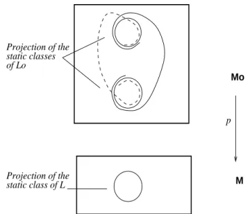
4-12 The extended static classes. . . 145
5 Examples 155 5-1 Riemannian Lagrangians. . . 155
5-2 Mechanic Lagrangians. . . 155
5-3 Symmetric Lagrangians. . . 156
CONTENTS v
5-4 Simple Pendulum. . . 156
5-5 The flat Torus Tn. . . 157
5-6 Flat domain for the β-function. . . 158
5-7 A Lagrangian with Peierls barrier h= +∞. . . 158
5-8 Horocycle flow. . . 160
6 Generic Lagrangians. 165 6-1 Generic Families of Lagrangians. . . 166
6-1.a Open. . . 169
6-1.b Dense. . . 170
7 Generic Lagrangians. 175 7-1 Generic Lagrangians. . . 176
7-2 Homoclinic Orbits. . . 188
Appendix. 195 A Absolutely continuous functions. . . 195
B Measure Theory . . . 197
C Convex functions. . . 198
D The Fenchel and Legendre Transforms. . . 199
E Singular sets of convex funcions. . . 203
F Symplectic Linear Algebra. . . 205
Bibliography. 207
Index. 213
Chapter 1
Introduction.
1-1 Lagrangian Dynamics.
LetM be a boundarylessn-dimensional complete riemannian manifold.
An (autonomous) Lagrangian on M is a smooth function L:T M →R satisfying the following conditions:
(a) Convexity: The Hessian ∂2L
∂vi∂vj(x, v), calculated in linear co- ordinates on the fiber TxM, is uniformly positive definite for all (x, v)∈T M, i.e. there is A >0 such that
w·Lvv(x, v)·w≥A|w|2 for all (x, v)∈T M and w∈TxM. (b) Superlinearity:
|v|→+∞lim
L(x, v)
|v| = +∞, uniformly onx∈M, equivalently, for all A∈Rthere is B∈Rsuch that
L(x, v) ≥A|v| −B for all (x, v)∈T M.
(c) Boundedness1: For allr≥0, ℓ(r) = sup
(x,v)∈T M,
|v|≤r
L(x, v) <+∞. (1.1) g(r) = sup
|w|=1
|(x,v)|≤r
w·Lvv(x, v)·w <+∞. (1.2)
The Euler-Lagrange equation associated to a lagrangian L is (in local coordinates)
d dt
∂L
∂v x,x) =˙ ∂L
∂x(x,x).˙ (E-L)
The condition (c) implies that the Euler-Lagrange equation (E-L) defines a complete flowϕtonT M(proposition 1-3.2), called the Euler-Lagrange flow, by setting ϕt(x0, v0) = xv(t),x˙v(t)
, where xv : R → M is the solution of (E-L) withxv(0) =x0 and ˙xv(0) =v0.
We shall be interested on coverings p:N → M of a compact man- ifold M and the lifted Lagrangian L = L◦dp : T N → R of a convex superlinear lagrangianL on M. The lagrangian L then satisfies (a)–(c) and its flow ψt is the lift ofϕt.
Observe that when we add a closed 1-form ω to the lagrangian L, the new lagrangian L+ω also satisfies the hypothesis (a)-(c) and has the same Euler-Lagrange equation asL. This can also be seen using the variational interpretation of the Euler-Lagrange equation (see 1-2.3).
1The Boundedness condition (c) is equivalent to the condition that the associ- ated hamiltonianH is convex and superlinear, see remark 1-4.2. This condition is immediate when the manifoldM is compact.
1-2. the euler-lagrange equation. 9
1-2 The Euler-Lagrange equation.
The action of a differential curve γ : [0, T]→M is defined by
AL(γ) = Z T
0
L(γ(t),γ˙(t))dt
One of the main problems of the calculus of variations is to find and to study the curves that minimize the action. Denote by Ck(q1, q2;T) the set of Ck-differentiable curves γ : [0, T] → M such that γ(0) = q1
and γ(T) =q2.
1-2.1 Proposition. If a curvex(t)in the spaceCk(q1, q2;T)is a critical point of the action functional onCk(q1, q2;T), thenxsatisfies the Euler- Lagrange equation
d
dtLv(x(t),x(t)) =˙ Lx(x(t),x(t))˙ (E-L) in local coordinates. Consequently, this equation does not depend on the coordinate system.
Proof: Choose a coordinate system (x1, . . . , xn) about x(t). Let h(t) a differentiable curve such that h(0) = h(T) = 0. Then for every ε, sufficiently small the curveyε=x+εhis onCk(q1, q2;T) and contained in the coordinate system. Define
g(ε) =AL(yε)
Then g has a minimum in zero and
ε→0lim
g(ε)−g(0)
ε = lim
ε→0
Z T 0
L(x+εh,x˙+εh)˙ −L(x,x)˙
ε dt
= Z T
0 ε→0lim
εLxh+εLvh˙ +o(ε)
ε dt
= Z T
0
Lxh+Lvh dt˙
= Z T
0
(Lx− dtdLv)h dt+LvhT
0
= Z T
0
(Lx− dtdLv)h dt.
Hence
0 = Z T
0
Lx(x(t),x(t))˙ − d
dtLv(x(t),x(t))˙
h dt,
for any function h ∈ Ck(0,0;T). This implies that x(t) satisfies the Euler Lagrange equation (E-L).
The Euler Lagrange equation is a second order differential equation on M, but the convexity hypothesis (Lvv invertible) implies that this equation can also be seen as a first order differential equation onT M:
˙ x=v,
˙
v= (Lvv)−1(Lx−Lvxv).
The associated vector fieldX onT M is called the lagrangian vector field and its flowϕt the lagrangian flow. Observe thatX is of the form
X(x, v) = (v,·).
1-2.2 Remark. It is possible to do the same thing in the spaceCT(p, q), the set of absolutely continuous curvesγ : [0, T]→Msuch thatγ(0) =p and γ(T) =q. A priori minimizers do not have to be differentiable and there are examples where they are not, see Ball & Mizel [4]. However
1-2. the euler-lagrange equation. 11
when the lagrangian flow is complete (cf. proposition 1-3.2), every ab- solutely continuous minimizers is C2 and satisfies the Euler-Lagrange equation. See Mather [46].
1-2.3 Remark. If we add a closed 1-form ω to the lagrangian L, the lagrangian L+ω also satisfies the hypothesis (a)-(c). Moreover, the action functionalAL+ω on a neighbourbood of a curveγ ∈Ck(x1, x2, T) satisfies
AL+ω(η) =AL(η) + I
γ
ω,
because the curve η is homologous to γ. Therefore, the critical points forAL+ωand forALare the same. This implies that the Euler-Lagrange equations for L and L+ω are the same. But since the values of AL+ω and AL are different, minimizers of these two actions may be different.
1-3 The Energy function.
The energy function of the lagrangianL is E:T M →R, defined by E(x, v) = ∂L
∂v(x, v)·v−L(x, v). (1.3) Observe that ifx(t) is a solution of the Euler-Lagrange equation (E-L), then
d
dtE(x,x) =˙ dtdLv−Lx
·x˙ = 0.
Hence E : T M → R is an integral (i.e. invariant function2) for the lagrangian flow ϕt and its level sets, called energy levels are invariant underϕt. Moreover, the convexity implies that
d
dsE(x, sv)|s=1 =v·Lvv(x, v)·v >0.
Thus
v∈TminxME(x, v) =E(x,0) =−L(x,0).
Write
e0:= max
x∈ME(x,0) =−min
x∈ML(x,0)>−∞, (1.4) by the superlinearity e0 >−∞, then
e0= min{k∈R|π :E−1{k} →M is surjective}. (1.5) By the uniform convexity, and the boundedness condition,
A:= inf
(x,v)∈T M
|w|=1
w·Lvv(x, v)·w >0,
and then using (1.1) and (1.2), E(x, v) =E(x,0) +
Z |v|
0 d
dsE x, s|v|v ds
≥ −ℓ(0) + 12 A|v|2. (1.6)
2The energy is invariant only forautonomous(i.e. time-independent) lagrangians.
1-3. the energy function. 13
Similarly, using (1.2),
E(x, v) ≤e0+g(|v|)|v|. (1.7)
Hence 1-3.1 Remark.
If k∈Rand K ⊆M is compact, thenE−1{k} ∩TKM is compact.
1-3.2 Proposition. The Euler-Lagrange flow is complete.
Proof: Suppose that ]α, β[ is the maximal interval of definition of t7→
ϕt(v), and −∞ < α or β < +∞. Let k = E(v). Since E(ϕt(v)) ≡ k, by (1.6), there is a >0 such that 0≤ |ϕt(v)| ≤afor α ≤t≤β. Since ϕt(v) is of the form (γ(t),γ˙(t)), thenϕt(v) remains in the interior of the compact set
Q:=
(y, w)∈T Md(y, x)≤a
|β−α|+ 1
, |w| ≤a+ 1 , wherex=π(v). The Euler-Lagrange vector field is uniformly Lipschitz on Q. Then by the theory of ordinary differential equations, we can extend the interval of definition ]α, β[ of t7→ϕt(v).
1-4 Hamiltonian Systems.
LetT∗M be the cotangent bundle ofM. Define the Liouville’s 1-form Θ on T∗M as
Θp(ξ) =p(dπ ξ) forξ∈Tp(T∗M),
whereπ :T∗M →M is the projection. The canonical symplectic form on T∗M is defined as ω=dΘ.
A local chart x = (x1, . . . , xn) of M induces a local chart (x,p) = (x1, . . . , xn;p1, . . . , pn) of T∗M writing p ∈ T∗M asp = Σi pi dxi. In these coordinates the forms Θ andω are written
Θ =p·dx=P
i
pidxi, ω=dp∧dx=P
i
dpi∧dxi.
Ahamiltonianis a smooth functionH:T∗M →R. Thehamiltonian vector field XH associated to H is defined by
ω(XH,·) =dH. (1.8)
In local charts, the hamiltonian vector field defines the differential equa- tion
˙
x= Hp,
˙
p=− Hx, (1.9)
whereHxand Hp are the partial derivatives ofH with respect tox and p. Letψtbe thehamiltonian flow. Observe that it preservesH, because
d
dtH =Hxx˙+Hpp˙= 0.
Moreover, it preserves the symplectic form ω, because3
d
dt(ψ∗tω) =LXHω =d iXHω+iXHω =d(dH) +iXH(0) = 0.
3LX is the Lie derivative, defined on forms η by LXη = diXη+iXdη, where iXη=η(X,·) is thecontractionbyX. The Lie derivative satisfiesLXη= dtdψt∗η|t=0, whereψt is the flow ofX.
1-4. hamiltonian systems. 15
We shall be specially interested in hamiltonians obtained by the Fenchel transform of a lagrangian:
H(x, p) = max
v∈TxM p v−L(x, v).
Observe thatH =E◦ L−1, whereE is the energy function (1.3) and L(x, v) = (x, Lv(x, v)) is the Legendre transform ofL. Moreover 1-4.1 Proposition. The Legendre transform L : T M → T∗M, L(x, v) = (x, Lv(x, v)) is a conjugacy between the lagrangian flow and the hamiltonian flow.
Proof: By corollary D.2, the convexity and superlinearity hypothesis imply that L =L∗∗ =H∗. So if p=Lv(x, v) then v =Hp(x, p). With this notation:
H(x, p) =v·Lv(x, v)−L(x, v) =E◦ L−1
=p·Hp(x, p)−L(x, Hp(x, p)).
ThusHx =−Lx, and the Euler-Lagrange equation
˙
x= dtd x =v = Hp,
˙
p= dtd Lv =Lx=−Hx, is the same as the hamiltonian equations.
1-4.2 Remark. Using thatL∗ =H and H∗ =L, from proposition D.2 in the appendix we obtain that the boundedness condition is equivalent to
(c) Boundedness: H=L∗ is convex and superlinear.
We say that an energy levelH−1(k) isregular, ifkis a regular value of H, i.e. dH(x, p)6= 0 whenever H(x, p) =k.
1-4.3 Proposition. Two hamiltonian flows restricted to a same regular energy level are reparametrizations of each other.
Proof: Suppose that H, G : T∗M → R are two hamiltonians with H−1(k) =G−1(ℓ) and k,ℓ are regular values forH and Grespectively.
Then, ifH(x, p) =k,
kerd(x,p)H =T(x,p)H−1(k) =T(x,p)H−1(k) = kerd(x,p)G.
Thus there exists λ(x, p)>0 such thatd(x,p)H=λ(x, p)d(x,p)G. Equa- tion (1.8) implies that XH =λ(x, p)XG whenH(x, p) =k.
We shall need the following estimate on the norm of the partial derivative Lv(x, v).
1-4.4 Lemma. There is a function f : [0,∞[→ R+ such that kLv(x, v)k ≤f(|v|) for all(x, v) ∈T M.
Proof: The convexity condition implies that the maximum in H(x, p) = max
w∈TxMp·w−L(x, w)
is attained atw=v0 withp=Lv(x, v0). SinceH(x, Lv(x, v)) =E(x, v), Lv(x, v)·w≤E(x, v) +L(x, w), ∀v, w∈TxM, ∀x∈M.
Applying this inequality to −w, we get that
Lv(x, v)·w≥ −E(x, v)−L(x,−w).
Thus using (1.6), (1.7) and (1.1), for |v| ≤r, we have kLv(x, v)k ≤ |E(x, v)|+ max{ |L(x, v)|,|L(x,−v)| }
≤max{|ℓ(0)|+12Ar2, e0+g(r)r}+|ℓ(r)|=:f(r).
1-5. examples. 17
1-5 Examples.
We give here some basic examples of lagrangians.
Riemannian Lagrangians:
Given a riemannian metric g = h·,·ix on T M, the riemannian la- grangian on M is given by thekinetic energy
L(x, v) = 12 kvk2x. (1.10) Its Euler-Lagrange equation (E-L) is the equation of the geodesics ofg:
D
dt x˙ ≡0, (1.11)
and its Euler-Lagrange flow is the geodesic flow. Its corresponding hamiltonian is
H(x, p) = 12kpk2x.
Analogous to the riemannian lagrangian is the Finsler lagrangian, given also by formula (1.10), but wherek·kxis aFinsler metric, i.e. k·kx
is a (non necessarily symmetric4) norm on TxM which varies smoothly onx∈M. The Euler-Lagrange flow of a Finsler lagrangian is called the geodesic flow of the Finsler metric k·kx.
Mechanic Lagrangians:
The mechanic lagrangian, also called natural lagrangian, is given by the kinetic energy minus the potential energy U :M →R,
L(x, v) = 12kvk2x−U(x). (1.12) Its Euler-Lagrange equation is
D
dtx˙ =−∇U(x),
4i.e. kλ vkx=λkvkx only forλ≥0
where Ddt is the covariant derivative and ∇U is the gradient of U with respect to the riemannian metric g, i.e.
dxU(v) =h∇U(x), vix for all (x, v) ∈T M.
Its energy function and its hamiltonian are given by the kinetic energy plus potential energy:
E(x, v) = 12kvk2x+U(x), H(x, p) = 12kpk2x+U(x).
Symmetric Lagrangians.
The symmetric lagrangians is a class of lagrangian systems which includes the riemannian and mechanic lagrangians. These are the la- grangians which satisfy
L(x, v) =L(x,−v) for all (x, v)∈T M. (1.13) Their Euler-Lagrange flow is reversible in the sense that ϕ−t(v) =
−ϕt(−v).
Magnetic Lagrangians.
If one adds a closed 1-form ω to a lagrangian, L(x, v) = L(x, v) + ωx(v), the Euler-Lagrange flow does not change. This can be seen by first observing that the solutions of the Euler-Lagrange equation are the critical points of the action functional on curves onC(x, y, T) (with fixed time interval and fixed endpoints). Since ω is closed, the action functional of Land L on C(x, y, T) differ by a constant and hence they have the same critical points.
But adding a non-closed 1-form to a lagrangian does change the Euler-Lagrange flow. We call amagnetic lagrangian a lagrangian of the form
L(x, v) = 12 kvkx+ηx(v)−U(x), (1.14)
1-5. examples. 19
wherek·kx is a riemannian metric,η is a 1-form onM withdη6= 0, and U :M → R a smooth function. If Y :T M → T M is the bundle map such that
dη(u, v) =hY(u), vi then the Euler-Lagrange equation of (1.14) is
D
dt x˙ =Yx( ˙x)− ∇U(x). (1.15) This models the motion of a particle with unit mass and unit charge under the effect of a magnetic field with Lorentz forceY and potential energyU(x). The energy functional is the same as that of the mechanical lagrangian but its hamiltonian changes because of the change in the Legendre transform:
E(x, v) = 12 kvk2x+U(x),
H(x, p) = 12 kp−A(x)k2x+U(x),
whereA:M →T M is the vector field given by ηx(v) =hA(x), vix. Twisted geodesic flows.
The twisted geodesic flows correspond to the motion of a particle under the effect of a magnetic field with no potential energy. This can be modeled as the Euler-Lagrange flow of a lagrangian of the formL(x, v) =
1
2kvk2x+ηx(v), wheredη6≡0. But the Euler-Lagrange equations depend only on the riemannian metric and dη. A generalization of these flows can be made using a non-zero 2-form Ω instead of dηand not requiring Ω to be exact. This is better presented in the hamiltonian setting.
Fix a riemannian metrich, iand a 2-form Ω onM. LetK :T T M → T M be the connection map Kξ = ∇x˙v, where ξ = dtd x(t), v(t)
. Let π : T M → M be the canonical projection. Let ω0 be the symplectic form inT M obtained by pulling back the canonical symplectic form via the Legendre transform associated to the riemannian metric, i.e.
ω0(ξ, ζ) =hdπ ξ , Kζi − hdπ ζ , Kξi.
The coordinates TθT M ∋ ξ ←→ (dπ ξ, Kξ) ∈ Tπ(θ)M ⊕Tπ(θ)M = H(θ)⊕V(θ) are the standard way of writing the horizontal and vertical components of a vector ξ ∈ TθT M for a riemannian manifold M (see Klingenberg [31]).
Define a new symplectic form ωΩ on T M by ωΩ=ω0+π∗Ω.
This is called a twisted symplectic structure on T M. Let H :T M →R be the hamiltonian
H(x, v) = 12kvk2x .
Consider the hamiltonian vector fieldXF corresponding to (H, ωΩ), i.e.
ωΩ XΩ(θ),·
=dH . (1.16)
Define Y :T M →T M as the bundle map such that
Ωx(u, v) =hY(u), vix. (1.17) The hamiltonian vector field XΩ(θ) ∈ TθT M is given by XΩ(θ) = (θ, Y(θ))∈H(θ)⊕V(θ). Hence the hamiltonian equation is
D
dt x˙ =Yx( ˙x),
recovering equation (1.15) with U ≡0, but where Ω doesn’t need to be exact.
IfH1(M,R) = 0, both approaches coincide, and any twisted geodesic flow is the lagrangian flow of a magnetic lagrangian of the formL(x, v) =
1
2 kvk2x+ηx(v), withdη = Ω. For example if N is a compact manifold Ω is a 2-form in N and M is the abelian cover or the universal cover of N; if Ω is not exact, then the corresponding twisted geodesic flow is a lagrangian flow on M but not on N (where it is locally a lagrangian flow). This lagrangian flow on M is actually the lift of the twisted geodesic flow on N.
1-5. examples. 21
Embedding flows:
There is a way to embed the flow of any bounded vector field on a lagrangian system. Given a smooth bounded vector fieldF :M →T M, let
L(x, v) = 12 kv−F(x)k2x. (1.18) SinceF(x) is bounded, then the lagrangianLis convex, superlinear and satisfies the boundedness condition. The lagrangian L on a fiber TxM is minimized at (x, F(x)), hence the integral curves of the vector field,
˙
x=F(x), are solutions to the Euler-Lagrange equation.
Chapter 2
Ma˜ n´ e’s critical value.
2-1 The action potential and the critical value.
We shall be interested on action minimizing curves with free time in- terval. Unless otherwise stated, all the curves will be assumed to be absolutely continuous. Forx, y∈M, let
C(x, y) ={γ : [0, T]→M|T >0, γ(0) =x, γ(T) =y}. Fork∈R define theaction potential Φk:M×M →R∪ {−∞}, by
Φk(x, y) = inf
γ∈C(x,y)AL+k(γ).
Observe that if there exists a closed curveγ on N with negative L+k action, then Φk(x, y) = −∞ for all x, y ∈ N, by going round γ many times.
Define thecritical level c=c(L) as
c(L) = sup{k∈R| ∃ closed curve γ withAL+k(γ)<0}.
Observe that the functionk7→Φk(x, y) is increasing. The superlinearity implies that L is bounded below. Hence there is k ∈ R such that
L+k≥0. Thus c(L) <+∞. Sincek7→ AL+k(γ) is increasing for any γ, we have that
c(L) = inf{k∈R|AL+k(γ)≥0∀closed curveγ}. 2-1.1 Proposition.
1. (a) For k < c(L), Φk(x, y) =−∞ for all x, y∈M. (b) For k≥c(L), Φk(x, y) ∈R for all x, y∈M.
2. For k≥c(L), Φk(x, z)≤Φk(x, y) + Φk(y, z), ∀x, y, z∈M.
3. Φk(x, x) = 0, ∀x∈M.
4. Φk(x, y) + Φk(y, x)≥0 ∀x, y∈M. Fork > c(L), Φk(x, y) + Φk(y, x)>0 if x6=y.
5. For k≥c(L) the action potential Φk is Lipschitz.
2-1.2 Remark. The action potential Φkis not symmetric in general, but items 2, 3, 4 imply that
dk(x, y) = Φk(x, y) + Φk(y, x)
is a metric for k > c(L) and a pseudo-metric for k=c(L) [i.e. perhaps dc(x, y) = 0 for some x6=y and c=c(L)].
Proof:
2. We first prove 2 for all k ∈ R. Since Φk(x, y) ∈ R∪ {−∞}, the inequality in item 2 makes sense for all k ∈ R. If γ ∈ C(x, y), η∈ C(y, z), thenγ∗η∈ C(x, z) and hence
Φk(x, z)≤AL+k(γ∗η)≤AL+k(γ) +AL+k(η).
Taking the infima onγ ∈ C(x, y) and η∈ C(y, z), we obtain 2.
2-1. the action potential and the critical value. 25
1. (a) If γ is a closed curve with AL+k(γ)<0 and γ(0) =z, then Φk(z, z)≤ lim
N→∞AL+k(γ∗· · · ∗N γ) = lim
N N AL+k(γ) =−∞. Forx, y∈M, item 2 implies that
Φk(x, y)≤Φk(x, z) + Φk(z, z) + Φk(z, y) =−∞.
Since the function k7→ Φk(x, y) is increasing, then item 1(a) fol- lows.
(b) Conversely, if Φk(x, y) = −∞ for some k ∈ R and x, y ∈ M, then
Φk(x, x)≤Φk(x, y) + Φk(y, x) =−∞.
Thus there isγ ∈ C(x, x) withAL+k(γ) <0. Thenk≤c(L). Ob- serve that the set{k∈R|AL+k(γ) <0 for some closed curve γ} is open. Hence Φk(x, y) = −∞ actually implies that k < c(L).
This proves item 1(b).
3. Let k ∈ R by the boundedness condition there exists Q > 0 be such that
|L(x, v) +k| ≤Q for|v| ≤2. (2.1) Now let γ : [0, ε]→ M be a differentiable curve with |γ˙| ≡1 and γ(0) =x. Then
Φk(x, x) ≤Φk(x, γ(ε)) + Φk(γ(ε), x)
≤AL+k γ|[0,ε]
+AL+k γ(t−ε)|[0,ε]
≤2Q ε.
Lettingε→0 we get that Φk(x, x)≤0. But the definition ofc(L) and the monotonicity ofk7→Φk(x, x) imply that Φk(x, x)≥0 for all k≥c(L).
5. Letk≥c(L). Givenx1, x2 ∈M we have that Φk(x1, x2)≤AL+k(γ)≤Q dM(x1, x2),
where γ : [0, d(x1, x2)] → N is a unit speed minimizing geodesic joiningx1 to x2 and Q >0 is from (2.1). If y1, y2 ∈ M, then the triangle inequality implies that
Φk(x1, y1)−Φk(x2, y2)≤Φk(x1, x2) + Φk(y2, y1)
≤Q[dM(x1, x2) +dM(y1, y2)].
Changing the roles of (x1, y1) and (x2, y2) we get item 5.
4. The first part of item 4 follows from items 2 and 3. Now suppose that k > c(L), x 6= y and dk(x, y) = 0. Let γn : [0, Tn] → M, γn ∈ C(x, y) be such that Φk(x, y) = limnAL+k(γn). We claim thatTn is bounded below.
Indeed, suppose that limnTn = 0. Let A >0, from the superlin- earity there isB >0 such thatL(x, v)≥A|v|−B, ∀(x, v)∈T M. Then
Φk(x, y) = lim
n
Z TN
0
L(γn,γ˙n) +k
≥lim
n A R
|γ˙|+ (k−B)Tn
=A dM(x, y)
LettingA→+∞ we get that Φk(x, y) = +∞which is false.
Now let ηn : [0, Sn] → M, ηn ∈ C(y, x) with limnAL+k(ηn) = Φk(y, x). Choose 0 < T < lim infnTn and 0 < S < lim infnSn. Then for c=c(L)< k,
Φc(x, x)≤lim
n AL+c(γn∗ηn)
≤lim
n AL+k(γn) + (c−k)T +AL+k(ηn) + (c−k)S
≤lim
n Φk(x, y) + Φk(y, x) + (c−k)(T +S)
≤(c−k)(T +S)<0, which contradicts item 3.
2-2. continuity of the critical value. 27
2-2 Continuity of the critical value.
2-2.1 Lemma. The function C∞(M,R)∋ψ7→c(L+ψ) is continuous in the topology induced by the supremum norm.
Proof: Suppose thatψn →ψand letcn:=c(L+ψn) andc:=c(L+ψ).
We will prove that cn→c.
Fix ε > 0. Since c−ε < c, by the definition of critical value there exists a closed curve γ : [0, T]→ M such that AL+ψ+c−ε(γ) <0, hence for all nsufficiently large
AL+ψn+c−ε(γ)<0.
Therefore fornsufficiently largec−ε < cn, and thusc−ε≤lim infncn. Since εwas arbitrary we have thatc≤lim infncn.
We show now that lim supncn ≤ c. Suppose that c < lim supncn. Take εsuch that
c < c+ε <lim supncn. (2.2) Since ψn→ψ, there exists n0 such that for alln≥n0,
−ε≤ψ−ψn≤ε. (2.3)
By (2.2), there existsm≥n0 such that c < c+ε < cm.
By the definition of critical value there exists a closed curveγ : [0, T]→ M such that
AL+ψm+c+ε(γ)<0, and hence using (2.3) we have
AL+ψ+c(γ)≤AL+ψm+c+ε(γ)<0,
which yields a contradiction to the definition of the critical value c.
This proof also shows that L7→ c(L) is continuous if we endow the set of lagrangians L with the topology induced by the supremum norm on compact subsets ofT M.
2-3 Holonomic measures.
Let Cℓ0 be the set of continuous functions f : T M → R having linear growth, i.e.
kfkℓ:= sup
(x,v)∈T M
|f(x, v)|
1 +kvk <+∞.
Let Mℓ be the set of Borel probabilities µon T M such that Z
T Mkvk dµ <+∞,
endowed with the topology such that limnµn=µ if and only if limn
Z
f dµn= Z
f dµ (2.4)
for all f ∈Cℓ0.
Let (Cℓ0)′ the dual of Cℓ0. ThenMℓ is naturally embedded in (Cℓ0)′ and its topology coincides with that induced by the weak* topology on (Cℓ0)′.
We shall see that this topology is metrizable. Let{fn}be a sequence of functions with compact support on Cℓ0 which is dense on Cℓ0 in the topology of uniform convergence on compact sets ofT M. Define a metric d(·,·) on Mℓ by
d(µ1, µ2) = Z
|v|dµ1− Z
|v|dµ2 +X
n
1 2n
1 cn
Z
fndµ1− Z
fndµ2 (2.5) wherecn= sup(x,v)|fn(x, v)|.
2-3.1Exercises:
1. Constructµ∈ Mℓ such thatR
|v|2dµ= +∞. 2. Show that the first term in (2.5) is necessary.
2-3. holonomic measures. 29
2-3.2 Proposition.
The metric d(·,·) induces the weak* topology on Mℓ⊂(Cℓ0)′. Proof: We prove thatd(·,·) generates the weak* topology onMℓ. Sup-
pose that Z
f dµn→ Z
f dµ, ∀f ∈Cℓ0. Given ε > 0, choose M > 0 such that P
m≥M 1
2m ·2 < ε, and choose N >0 such that
Z
fmdµn− Z
fmdµ
< ε, for 0≤m≤M, n≥N;
Z
|v|dµn− Z
|v|dµ
< ε, forn≥N.
Since kfnck∞
n = 1, then for n > N we have that d(µn, µ)≤ε+ PM
m=1 1
2m ·ε+ P
m≥M+1 1
2m ·2·kfcmmk = 3ε.
Thusd(µn, µ)→0.
Now suppose that d(µn, µ)→0. Let Km be compact sets such that Km⊂Km+1 and that T M =∪Km. Then
Z
Km
f dµn−→
Z
Km
f dµ, ∀f ∈Cℓ0, ∀m;
Z
|v|dµn−→
Z
|v|dµ.
This implies that
n→∞lim Z
T M−Km
|v|dµn = Z
T M−Km
|v|dµ, ∀m. (2.6) Given ε >0, choosem(ε)>0 such that
Z
T M−Km(ε)
(1 +|v|)dµ < ε 4,
and N such that Z
T M−Km(ε)
(1 +|v|)dµn< ε
2, ∀n > N.
Fix f ∈Cℓ0. Choose N >0 such that
Z
Km(ε)
f dµn− Z
Km(ε)
f dµ
< ε, ∀n > N.
Then Z
T M−Km(ε)
|f| dµn≤ kfkℓ
Z
T M−Km(ε)
(1 +|v|)dµn≤ kfkℓ
ε
2, ∀n > N.
Using a similar estimate for µwe obtain that
Z
f dµn− Z
f dµ
≤ε+kfkℓ (2ε+ ε4).
Ifγ : [0, T]→M is a closed absolutely continuous curve, letµγ∈ Mℓ
be defined by Z
f dµγ = 1 T
Z T 0
f γ(t),γ˙(t) dt
for all f ∈Cℓ0. Observe thatµγ ∈ Mℓ because if γ is absolutely contin- uous then R
|γ(t)˙ |dt <+∞. LetC(M) be the set of such µγ’s and let C(M) be its closure in Mℓ. Observe that the set C(M) is convex. We call C(M) the set ofholonomic measureson M.
2-4. invariance of minimizing measures. 31
2-4 Invariance of minimizing measures.
Given a Borel probability measureµinT M define itsaction by AL(µ) =
Z
T M
L dµ.
Since by the superlinearity the lagrangian L is bounded below, this action is well defined. Observe thatL /∈Cℓ0 and that AL(µ) = +∞ for someµ∈ Mℓ (see exercise 2-3.1).
Let M(L) be the set ofϕt-invariant probabilities onT M. 2-4.1 Theorem (Ma˜n´e [38], prop. 1.1, 1.3, 1.2).
1. M(L)⊆ C(M)⊆ Mℓ. 2. If µ∈ C(M) satisfies
AL(µ) = min{AL(ν)|ν ∈ C(M)}, then µ∈ M(L).
3. If M is compact and a∈R, then the set {µ∈ C(M)|AL(µ)≤a} is compact.
Observe that item 3 implies the existence of a minimizer as in item 2.
The inclusionM(L)⊆ C(M) follows from Birkhoff’s ergodic theorem and the fact that C(M) is convex. Takingf =kvkin equation (2.4) we see that Mℓ is closed, so that C(M)⊆ Mℓ.
Proof of item 2-4.1.3:
Since C(M) is closed, it is enough to prove that the set A(a) :=
µ∈ Mℓ|AL(µ)≤a
is compact in Mℓ. First we prove that A(a) is closed. Let k >0 and defineLk:= min{L, k}. Let
Bk:=
µ∈ Mℓ|R
Lkdµ≤a .
Since Lk ∈ Cℓ0, then Bk is closed in Mℓ. Since A(a) = ∩k>0Bk, then A(a) is closed.
In order to prove the compactness, consider a sequence{µn} ⊂ A(a).
Applying the Riesz’ theorem B.1, taking a subsequence we can assume that there exists a measure µon the Borel σ-algebra ofT M such that
Z
fi dµn−→
Z
fi dµ, (2.7)
for every fi in the sequence used for the definition of d(·,·). Approxi- mating the function 1 by the functionsfi we see thatµis a probability.
Approximating Lk by functionsfi we have that Z
Lk dµ= lim
n
Z
Lkdµn≤lim inf
n
Z
L dµn≤a.
Lettingk↑+∞, by the monotone convergence theorem, we get that
AL(µ)≤a. (2.8)
LetB >0 be such that |v|< L(x, v) +B for all (x, v)∈T M. Then Z
|v|dµ≤AL(µ) +B ≤a+B <+∞. (2.9) So thatµ∈ Mℓ.
We now prove that limnR
|v| dµn −→ R
|v| dµ. Let ε > 0. By adding a constant we may assume that L >0. Choose r >0 such that L(x, v)> a ε−1|v|for all|v|> r. Then
Z
|v|>r|v|dµn≤ ε a
Z
|v|>r
L dµn≤ ε a
Z
L dµn≤ε.
Similarly, by (2.8),
Z
|v|>r|v|dµ≤ε.
2-4. invariance of minimizing measures. 33
From (2.7) we obtain that there is N >0 such that
Z
|v|≤r|v|dµ− Z
|v|≤r|v|dµn
< ε, forn > N.
Adding these inequalities we get that
Z
|v|dµn− Z
|v|dµ ≤3ε.
The proof of item 2-4.1.2 requires some preliminary results which we present now. Item 2-4.1.2 is proved at the end of the section.
The following proposition is needed to show that the minimum of the action inC(M) is the same as the minimum on C(M).
2-4.2 Proposition.
Given µ∈ C(M), there are µηn ∈ C(M) such that µηn →µand limn
Z
L dµηn = Z
L dµ.
2-4.3 Remark. The statement of proposition 2-4.2 is not trivial. It is easy to see that the function AL:C(M) →R is always lower semicon- tinuous (see the last argument of the proof of 2-4.2), but in general it is not continuous. It is possible to give a sequence µγn ∈ C(M) such that µγn → µ in C(M) but lim infnAL(µγn) > AL(µ) for a quadratic lagrangian L.
This can be made by calibrating the high speeds in γn so that R
[|v|>R]|v|dµγn → 0 but a := lim infnR
[|v|>R]L dµγn > 0. Then the limit measure µ will have support on [|v| ≤ R] and “will not see” the remnantaof the action.
Proof: Let A > 1 and let γ : [0, T] → M be a closed absolutely con- tinuous curve. We reparametrizeγ to a curve η: [0, S]→ M such that
˙
η= ˙γ when|γ˙|< Aand ˙η = |˙γγ|˙ A when|γ˙|> A. So that|η˙| ≤A. Write η(s(t)) =γ(t), w(s) =|η(s)˙ |andv(t) =|γ(t)˙ |. We want
Z s(t) 0
w(s)ds= Z t
0
v(t)dt,
so that
s′(t) = v(t) w(s(t)) =
(1 when v(t)≤A.
v(t)
A when v(t)≥A.
Then
S(T) = Z
[v(t)≤A]
dt+ Z
[v(t)≥A]
v(t) A dt, S(T)
T =µγ([|v| ≤A]) + Z
[|v|≥A]
|v| A dµγ,
S(T)
T −1 ≤
Z
[|v|>A]
dµγ+ Z
[|v|≥A]
|v| A dµγ
≤2 Z
[|v|>A]|v|dµγ. (2.10)
Suppose that f : T M → R is µη-integrable. Since dsdt = v(t)A when v(t)> Athen
Z
[|γ(t(s))|>A]˙
f(η(s),|γ(t(s))γ(t(s))|˙˙ A)ds= Z
[|˙γ(t)>A]
f γ(t),|˙γ(t)γ(t)|˙ A|γ(t)˙ | A dt.
2-4. invariance of minimizing measures. 35
ThenZ
f dµη = 1 S(T)
Z
f(η(s),η(s))˙ ds
= 1
S(T)
" Z
[|γ|≤A]˙
f(γ(t),γ˙(t))dt+ Z
[|˙γ(t(s))|>A]
f η(s),|˙γ(t(s))γ(t(s))|˙ A ds
#
= T
S(T)
" Z
[|v|≤A]
f(v)dµγ(v) + Z
[|v|>A]
f |v|v A|v| A dµγ
#
ForA >1 big enough, Z
[|v|>A]|v|dµγ< ε < 14. (2.11) Define
fA(v) :=
(f(v) if|v| ≤A, f |v|v A|v|
A if|v|> A.
Then Z
f dµη = S(TT ) Z
fAdµγ. (2.12)
Observe that from (2.10) and (2.11), we have that
S(TT ) −1≤4ε. (2.13) Then
Z
f dµη− Z
fAdµγ
≤S(TT )−1 Z
|fA|dµγ ≤4ε Z
|fA|dµγ. (2.14) Ifkfk∞≤1, then
Z
|fA|dµγ ≤ Z
[|v|≤A]|f|dµγ+ Z
[|v|>A]|f−fA|dµγ
≤1 + Z
[|v|>A]
|v|
A dµγ ≤1 +ε.
Z
f dµη − Z
f dµγ =
S(TT )
Z
fAdµγ− Z
f dµγ
≤S(TT )−1 Z
|fA|dµγ+ Z
|f −fA|dµγ
≤4ε(1 +ε) +ε≤6ε.
Also, using (2.14),
Z
|v|dµη− Z
|v|dµγ
=S(TT ) −1 Z
|v|dµγ ≤4ε Z
|v|dµγ. Hence
dMℓ(µη, µγ)≤6ε Z
(|v|+ 1)dµγ. (2.15) Now let µ∈ C(M). Let
K := 1 + Z
(|v|+ 1)dµ. (2.16) ForR >0, define
LR(v) :=
(L(v) if|v| ≤R.
L |v|v R|v|
R if|v|> R.
Claim: IfE(v)>0 for all |v| ≥R, then
LR(v)≤L(v) for all v∈T M.
Proof:
If |v| ≤R thenLR(v) =L(v). Suppose that |v|=R. Fors≥1 let f(s) :=L(sv)−LR(sv) =L(sv)−sL(v).
It is enough to prove thatf(s)≥0 for all s≥1. We have f′(s) =v·Lv(sv)−L(v)
f′′(s) =v·Lvv(sv)·v >0.
2-4. invariance of minimizing measures. 37
We have that f(1) = 0,f′(1) = E(v) >0, f′′(s)>0 for all s≥1. This implies thatf(s)≥0 for all s≥1.
♦ Given N >0, chooseR=R(N)>1 such that
E(v)>0 if|v| ≥R and
Z
|v|>R|v|dµ < N1. (2.17) Observe LR(N) has linear growth. ChooseµγN ∈ C(M) such that
dMℓ(µγN, µ)< N1, (2.18) Z
LR(N)dµγN ≤ Z
LR(N) dµ+ N1, and
Z
[|v|≤R(N)]|v|dµγN ≥ Z
[|v|≤R(N)]|v|dµ− N1. (2.19) ThenZ
(|v|+ 1)dµγN ≤K from (2.16) and (2.18), (2.20) Z
[|v|>R(N)]|v|dµγN < N3 from (2.17), (2.18) and (2.19). (2.21) ConstructηN as above forγN andA=R(N). Then from (2.11), (2.15), (2.20) and (2.21),dMℓ(µηN, µγN)< 18N K. From (2.18),
dMℓ(µηN, µ)< 18N K+N1.
ThusµηN −→N µinC(M). Moreover, from (2.12), (2.13), (2.11) and the claim,
Z
L dµηN = S(TTN
N)
Z
LR(N)dµγN ≤ S(TTNN) Z
LR(N) dµ+N1
≤ 1 +12N Z
L dµ+ N1
.
Hence
lim sup
N
Z
L dµηN ≤ Z
L dµ.
Fix R >0 such that E >0 on |v|> R. ThenLR has linear growth and by the claimLR≤L. Therefore
lim inf
N
Z
L dµηN ≥lim
N
Z
LRdµηN = Z
LRdµ.
LettingR ↑+∞, by the dominated convergence theorem we get that lim inf
N
Z
L dµηN ≥ Z
L dµ.
Given x, y∈M, define
S(x, y;T) := inf
γ∈CT(x,y)AL(γ).
Observe that S(x, y;T) > −∞ because L is bounded below. If γ ∈ Cac([0, T], M), define
S+(γ) :=AL(γ)−S(γ(0), γ(T);T).
The absolutely continuous curves γ with S+(γ) = 0 are called Tonelli minimizers. Observe that a Tonelli minimizer is a solution of (E-L).
Given γ1, γ2 ∈ Cac([0, T], M), the absolutely continuous distance d1(γ1, γ2) is defined by
d1(γ1, γ2) := sup
t∈[0,T]
d γ1(t), γ2(t) +
Z T 0
dT M [γ1(t),γ˙1(t)],[γ2(t),γ˙2(t)]
dt.
2-4.4 Proposition. Given a compact subsetK ⊆M and givenC,ε >0 there existδ >0such that ifγ : [0, T]→M is absolutely continuous and satisfies
2-4. invariance of minimizing measures. 39
i. 1≤T ≤C.
ii. AL(γ)≤C.
iii. S+(γ)≤δ.
Then either γ([0, T])∩K = or there exists a Tonelli minimizer γ0 : [0, T]→M such that d1(γ0, γ)≤ε.
Proof: If such δ does not exists then there is a sequence γn ∈ Cac([0, Tn], M) such that γn([0, Tn])∩K 6=, 1≤Tn≤C,S+(γn)→0, AL(γn)≤C and d1(γn, η)≥εfor any Tonelli minimizer η.
Adding a constant we can assume that L > 0. Let B > 0 be such thatL(x, v) >|v| −B for all (x, v) ∈T M. Chooses0 ∈[0, Tn] such that γn(s0)∈K. Then
d(K, γn(t))≤d(γn(s0), γn(t))≤ Z
[s0,t]|γ˙n|
≤ Z
[s0,t]
L(γn,γ˙n) +B
≤C+B C.
LetQ:={y∈M|d(y, K)≤C+B C }. Then we have thatγn([0, Tn])⊆ Q.
We can assume that Tn →T, γn(0)→ x∈Q and γn(Tn) →y ∈Q.
Moreover, we can assume that Tn ≡ T,γn(0) ≡ x and γn(T) ≡y. By theorem 3-1.2, the set A(b) =
γ ∈ CT(x, y)|AL(γ)≤b is compact in the C0-topology. Then we can assume that there is γ0 ∈ CT(x, y) such that γn → γ0 in the C0-topology. Since the action functional is lower semicontinuous, then AL(γ0) ≤ lim infnAL(γn) = S(x, y;T), because S+(γn) → 0. Thus γ0 is a Tonelli minimizer. Moreover, we have that AL(γn)→AL(γ0). By proposition 3-1.3, γn→γ0 in the d1-topology.
Let H:=
h :T M →R kfk∞≤1, [h]Lip≤1, h with compact support ,
where
[h]Lip= sup
(x,v)6=(y,w)
|h(x, v)−h(y, w)| dT M (x, v),(y, w) is the smallest Lipschitz constant for h.
2-4.5 Corollary.
Given h ∈ H and C > 0 there exist δ = δ(C, h) > 0 such that if γ : [0, T]→M satisfies conditions 2-4.4.i, 2-4.4.ii, 2-4.4.iii then
I
γ
h− I
γ
h◦ϕ1
≤5. (2.22)
Proof: Let K = π supp(h)∪ϕ−1(supp(h))
. Given C >0 and ε >0 let δ = δ(C, ε) > 0 and A > 0 be given by proposition 2-4.4 then if γ : [0, T] → M satisfies conditions 2-4.4.i, 2-4.4.ii, 2-4.4.iii we have that either γ([0, T])∩K = , or we can take γ0 minimizing such that d1(γ0, γ)≤ε.
Observe that ifγ([0, T])∩K =, thenh(γ,γ˙)≡0 andh◦ϕ1(γ,γ˙)≡ 0. This implies (2.22). Suppose then thatd1(γ0, γ) ≤ε.
We have that
I
γ
h− I
γ0
h
≤[h]Lipd1(γ, γ0)≤1·1·ε,
where [h]Lip is the smallest Lipschitz constant of h. Let Q(h) :=
ϕ−1(supp(h)), then
I
γ
h◦ϕ1− I
γ0
h◦ϕ1
≤[h]Lip[ϕ1|Q(h)]Lipd1(γ, γ0)≤1·[ϕ1|Q(h)]Lip·ε.
Since γ0 is a solution of (E-L), we have that
I
γ0
h− I
γ0
h◦ϕ1 =
Z T 0
h γ0(t),γ˙0(t)
−h γ0(t+ 1),γ˙0(t+ 1) dt
≤ Z 1
0 |h(γ0,γ˙0)|dt+ Z T+1
T |h(γ0,γ˙0)|dt≤2.
2-4. invariance of minimizing measures. 41
Hence
I
γ
h− I
γ
h◦ϕ1
≤ε 1 + [ϕ1|Q(h)]Lip + 2.
Proof of item 2-4.1.2:
Observe that to prove thatµ is invariant it is enough to prove that Z
h dµ= Z
h d(ϕ∗1µ) for allh∈ H. (2.23) By proposition 2-4.2, there exists a sequence µγn ∈ C(M) such that µγn →µ and
limn AL(µγn) =AL(µ) = min
AL(ν)|ν∈ C(M) =:k. (2.24) Let Tn be a period of the curve γn : R→ M. Take an integer N > 0.
By joining a constant curve if necessary, we can assume that every Tn is a multiple of N and that limn→∞Tn= +∞. Given C >0 let
Bn(C) :=
j∈N|1≤j≤ TNn, AL(γn,j)≥C , where
γn,j :=γn|[jN,(j+1)N].
By the superlinearity L is bounded below, adding a constant we can assume that L >0. Then we can assume that
AL(µγn) = 1 Tn
Z Tn
0
L(γn,γ˙n)dt≤2k ∀n.
Hence
2k Tn≥ X
j∈Bn(C)
AL(γn,j)≥C#Bn(C).
Thus #Bn(C)
Tn ≤ 2k
C. (2.25)