Notes on Information Theory and Coding.

Notes on Information Theory and Coding.

Henk Bruin December 15, 2020

1 Automata

In this section we discuss Turing machines and variations of it, and ask the question what languages they can recognize or generate. The terminology is not entirely consis- tent in the literature, so some of the below notions may be called differently depending on which book you read.

1.1 Turing Machines

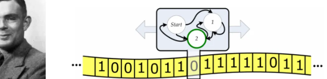
A Turing machine is a formal description of a simple type of computer, named after the British mathematician Alan Turing (1912-1954). He used this in theoretic papers to explore the limits what is computable by computers and what is not. For us, the size of a Turing machine that can recognize words in a language L(X), or reject words that don’t belong to L(X), is a measure for how complicated a subshift is. In fact, a subshift is called regularly enumerablein the Chomsky hierarchy if its language can be recognized by a Turing machine.

Figure 1: Alan Turing (1912-1954) and his machine.

A Turing machine has the following components:

• A tape on which the input is written as a word in the alphabet {0,1}.

• A reading device, that can read a symbol at one position on the tape at the time.

It can also erase the symbol and write a new one, and it can move to the next or previous position on the tape.

• A finite collection of states S₁, . . . , S_N, so N is the size of the Turing machine.

Each state comes with a short list of instructions:

– read the symbol;

– replace the symbol or not;

– move to the left or right position;

– move to another (or the same) state.

One state, sayS₁, is theinitial state. One (or several) states arehalting states.

When one of these is reached, the machine stops.

Example 1.1. The following Turing machine rejects tape inputs that do not belong to the language of the Fibonacci shift. Let s be the symbol read at the current position of the tape, starting at the first position. We describe the states:

S₁: If s= 0, move to the right and go to State S₁. Ifs= 1, move to the right and go to State S₂.

S₂: If s = 0, move to the right and go to State S₁. If s= 1, go to State S₃. S₃: Halt. The word is rejected, see Figure 2.

S₁ S₂ S₃

s= 1 move right

s= 0 move right s= 0

move right

s= 1

Figure 2: A Turing machine accepting words from the Fibonacci shift.

Rather than an actual computing devise, Turing machines are a theoretical tool to study which types of problems are in principle solvable by a computer. For instance, we call a sequence (xn)n≥0 automatic if there is a Turing machine that produces xn

hen the binary expansion of n is written on the input tape. A number is automatic if its digits form an automatic sequence. Given that there are only countably many Turing machines, there are only countably many automatic numbers. Most reals are not automatic: no algorithm exists that can produce all its digits.

Another question to ask about Turing machines, or any computer program in gen- eral, is whether it will stop in finite time for a given input. This is thehalting problem.

Using an advanced version of the Russell paradox, Turing proved in 1936 [28] that a general algorithm to solve the halting problem for all possible program-input pairs can- not exist. However, in theory it is possible to create a universal Turing machine that does the work of all Turing machines together. Quoting Turing [28, page 241-242]:

It is possible to invent a single machine which can be used to compute any computable sequence. If this machine U is supplied with the tape on the beginning of which is written the string of quintuples separated by semicolons of some computing machine M, then U will compute the same sequence as M.

For thisU doesn’t need to combine the programs of the countably many separate Turing machine. Instead, the separate Turing machines M are to be encoded on the tape in some standardized way, and they will be read by U together with the input of for U. The program of U then interpret M and executes it. Universal Turing machines didn’t stay theoretical altogether. Shannon posed the question how small universal Turing machines can be. Marvin Minsky [19] constructed a version on a four-letter alphabet with seven states. Later construction emerged from cellular automata. This was improved to a 3-letter alphabet by Alex Smith in 2007, but his prove is in dispute.

A smaller alphabet is impossible [20]¹.

Exercise 1.2. Suppose two positive integers m and n are coded on a tape by first putting m ones, then a zero, then n ones, and then infinitely many zeros. Design Turing machines that compute m+n, |m−n| and mn so that the outcome is a tape with a single block of ones of that particular length, and zeros otherwise.

1.2 Finite Automata

A finite automaton (FA) is a simplified type of Turing machine that can only read a tape from left to right, and not write on it. The components are

M ={Q,A, q0, q,f} (1)

where

Q = collection of states the machine can be in.

A = the alphabet in which the tape is written.

q0 = the initial state in Q.

H = collection of halting states in Q; the FA halts when it reaches one.

f = is the rule how to go from one state to the next when reading a symbol a∈ A on the tape. Formally it is a function Q× A →Q.

A language is regular if it can be recognized by a finite automaton.

Example 1.3. The even shift is recognized by the following finite automaton with Q= {q₀, q₁, q₂, q₃} with initial state q₀ and final states q₂ (rejection) and q₃ (acceptance).

The tape is written in the alphabet A={0,1, b} where b stands for a blank at the end of the input word. The arrow q_i →q_j labeled a∈ A represents f(q_i, a) = q_j.

1This proof by Morgenstern is based on an unpublished result by L. Pavlotskaya from 1973.

q₃

q₂ q₁

q₀

1

1 0

0

b b

Figure 3: Transition graph for a finite automaton recognizing the even shift.

This example demonstrates how to assign a edged-labeled transition graph to a finite automaton, and it is clear from this that the regular languages are precisely the sofic languages.

It is frequently easier, for proofs or constructing compact examples, to allow finite automata with multiple outgoing arrows with the same label. So, if we are in state q, read symbol a on the input tape, and there is more than one outgoing arrow with label a, then we need to make choice. For computers, making choices is somewhat problematic - we don’t want to go into the theoretical subtleties of random number generators - but if you take the viewpoint of probability theory, you can simply assign equal probability to every valid choice, and independent of the choices you may have to make elsewhere in the process. The underlying stochastic process is then a discrete Markov process.

Automata of this type are called non-deterministic finite automata (NFA), as opposed to deterministic finite automata (DFA), where never a choice needs to be made. A word is accepted by an NFA if there is a positive probability that choices are made that parse the word until the end without halting or reaching a rejecting state.

We mention without proof (see [13, page 22] or [2, Chapter 4]):

Theorem 1.4. Let L be a language that is accepted by a non-deterministic finite au- tomaton. Then there is a deterministic finite automaton that accepts L as well.

Corollary 1.5. Let w^R=w_n. . . w₁ stand for the reverse of a word w=w₁. . . w_n. If a languageL is recognized by a finite automaton, then so is its reverse L^R={w^R:w∈ L}.

Proof. Let (G,A) the edge-labeled directed graph representing the FA for L. Reverse all the arrows. Clearly the reverse graph (G^R,A) in which the directions of all arrows are reversed and the final states become initial states and vice versa, recognizes L^R. However, even if in G, every outgoing arrow has a different label (so the FA is deter- ministic), this is no longer true for (G^R,A). But by Theorem 1.4 there is also an DFA that recognizes L^R.

Sometimes it is easier, again for proofs or constructing compact examples, to allow finite automata to have transitions in the graph without reading the symbol on the

q₃

q2

q1

q0

1

2 b

0

1 2

b b

2 q₂ q₁

q₀ 0

2 1

Figure 4: Finite automata recognizing L ={0^k1^l2^m :k, l, m≥0}.

input take (and moving to the next symbol). Such transitions are called -moves.

Automata with -moves are almost always non-deterministic, because if a state q has an outgoing arrow with label aand an outgoing arrow with label , and the input tape reads a, then still there is the choice to follow that a-arrow or the-arrow.

Example 1.6. The follow automata accept the language L = {0^k1^l2^m : k, l, m ≥ 0}, see Figure 4. The first is with-moves, and it stops when the end of the input is reached (regardless which state it is in). That is , if the FA doesn’t halt before the end of the word, then the word is accepted. The second is deterministic, but uses a blank b at the end of the input. In either case q0 is the initial state.

Again without proof (see [13, page 22]):

Theorem 1.7. LetL be a language that is accepted by a finite automaton with-moves.

Then there is a non-deterministic finite automaton without -moves that accepts L as well.

A deterministic finite automaton with output (DFAO) is an septuple

M_O={Q,A, q₀, H, f, τ,B}, (2)

where the first five components are the same as for an FA in (1), and τ :Q→ B is an output function that gives a symbol associated to each state inQ. It can be the writing device for a Turing machine. For a word w∈ A^∗, we let τ(q₀, w) :=t(q) be the symbol that is read off when the last letter of w is read (or when the automaton halts).

The following central notion was originally due to B¨uchi [4], see also the monograph by Allouche & Shallit [2].

Definition 1.8. Let A ={0,1, . . . , N−1}, and let[n]A denote the integer n expressed in base N. A sequence x∈ B^N is called an N-automatic sequence ifx_n=τ(q₀,[n]_A) for all n ∈N.

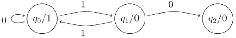
Example 1.9. The automaton in Figure 5 assigns the symbol 1 to every word w ∈ L(X_even) of the one-sided even shift and the symbol 0 to words w∈ {0,1}^N\ L(X_even).

The output functionτ :Q→ {0,1} is indicated by the second symbol at each state. The only halting state is q₃.

q₂/0 q₁/0

q₀/1

1

1 0

0

Figure 5: The DFAO for the even shift.

As such, the sequence x∈ {0,1}^N defined as x_n=

(1 n contains only even blocks of 1 in its binary expansion, 0 otherwise,

is an automatic sequence.

All sequence that are eventually periodic are automatic. In [2, Section 5.1], the Thue-Morse sequenceρTM= 0110 1001 10010110 10. . . is used as an example of an auto- matic sequence, because of its characterization asx_n = #{1s in the binary expansion of n−

1}mod 2, see Figure 6.

q₀/0 q₁/1

1

1

0 0

Figure 6: The DFAO for the Thue-Morse sequence.

Sturmian sequences are in general not; only if they are of the form x_n = bnα+ βcmodN for some α ∈ Q, see [1]. Some further results on automatic sequences are due to Cobham. The first is Cobham’s Little Theorem see [3, 5].

Theorem 1.10. The fixed point ρ of a substitution χ on A = {0, . . . , N −1} is an N-automatic sequence, and so is ψ(ρ) for any substitution ψ :A → B^∗.

The other is Cobham’s Theorem see [5, 15].

Theorem 1.11. If 2 ≤ M, N ∈ N are multiplicative independent, i.e., ^log_logN^M ∈/ Q, then the only sequences which are both M-automatic and N-automatic are eventually periodic.

Since all automatic sequence can basically written as in Theorem 1.10 (cf. [17]), this gives retrospectively information on substitution shifts, see Durand [6, 8, 7]

2 Data Compression

The wish to shorten texts is as old as writing itself. For example, tomb stones were seldom large enough to contain the intended message, so people resorted to (standard) abbreviations, see Figure 7. In the middle ages, vellum was expensive (it still is), so also here a variety of abbreviations was in use.

G(aius) Lovesius Papir(ia) (tribu) Inc(i)p(it) vita sci (= sancti) Cadarus Emerita mil(es) Martini episcopi et confessor(is).

Leg(ionis) XX V(aleriae) V(ictricis) Igitur Martinus Sabbariae

an(norum) XXV stip(endiorum) IIX Pannoniaru(m) oppido oriundus fuit, Frontinius Aquilo h(eres) sed intra Italiam Ticini altus e(st).

f(aciendum) c(uravit) parentibus secundum saeculi . . .

Figure 7: A Roman tombstone and Carolingian manuscript.

Naturally, writing itself is a means of coding messages, but over the years other methods of coding have been developed for special purposes, such as data compression, storage and transmission by computers (including bar-codes and two-dimensional bar- codes), for secrecy and many other needs.

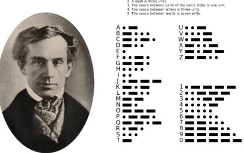
In 1821, Louis Braille developed the system of now named after him, after an earlier scheme that Charles Barbier devised for military use (Napoleon wanted a method for his soldiers to communicate in silence and without (day)light). Braille, who was a teacher at the Royal Institute for the Blind in Paris, designed his code of raised dots

in 2×3-cells that you can feel sliding your finger over the paper. There is a version of Braille, designed by Abraham Nemeth in 1952 (but with later revisions), intended to read mathematical texts. Compared to Braille, some symbols are coded differently (see Figure 8) and for more complicated symbols or expressions multiple six-dot patterns are combined.

Figure 8: Louis Braille (1809 – 1852) and his code.

When paper eventually became cheap and widely available in the 19th century, data compression of this sort wasn’t important anymore, but stenography (for taking speedy dictation or making eye-witness reports to be worked out in full later) was probably the most common form of data compression. With the advent of telegraphy and radio, there as a new reason to compress messages again. In Morse code (see Figure 9), the codes of the most frequently used letters are the shortest.

Morse code was developed in 1836 by Samuel Morse for telegraph² (and after its invention also radio) communication. It encodes every letter, digit and some punctua- tion marks by strings of short and long sounds, with silences between the letters, see Figure 9.

The lengths of the codes were chosen to be inverse proportional to the frequency the letters in the English language, so that the most frequent letter, E and T, get the shortest codes•and ••••, also to see that for other languages than English, Morse code is not optimal. This is one of the first attempts at data compression. The variable length of codes means, however, that Morse code is not quite a sliding block code.

Mechanization of the world increased the need for coding. The first computers in the middle of the 20th century were used for breaking codes in WWII. A little later, Shannon thought about optimizing codes for data transmission, naturally for

2In fact, Morse collaborated with Joseph Henry and Alfred Vail on the development of the telegraph, and they were not the only team. For example, in G¨ottingen, Gauß and Weber were working on early telegraph and telegraph codes since 1833.

Figure 9: Samuel Morse (1791 – 1872) and his code.

telegraph and telephone usage, see Section 2. But he was visionary enough to imagine that computers would soon become the main purpose of coding. In fact, he would see a large part of his predictions come true because he lived until 2001. The digital representation of text, that is representing letters as strings of zeros and ones, was standardized in the 1960s. ASCII stands for American Standard Code for Information Interchange. Developed in 1963, it assigns a word in {0,1}⁷ to every symbol on the keyboard, including several control codes such as tab, carriage return, most of which are by now obsolete. These seven digit codes allow for 2⁷ = 128 symbols, and this suffices for most purposes of data transmission and storage. Different versions were developed for different countries and makes of computers, but as in Braille, a text is coded in symbol strings, letter by letter, or in other words by a sliding block code of window size 1.

By this time bank transactions started to be done by telephone line, from computer to computer, and cryptography became in integral part of commerce, also in peace- time. Sound and music recordings became digital, with digital radio and CD- and DVD-players, and this cannot go without error correcting codes. For CD’s, a cross interleaved Reed-Somolon code is used, to correct errors that are inevitably caused by micro-scratches on the disc. CDs are particularly prone to burst errors, which are longer scratches in the direction of the track, which wipe out longer strings of code. For this reason, the information is put twice on the disc, a few seconds apart (this is what the

“interleaved” stands for), which causes the little pause before a CD starts to play.

2.1 Shannon’s Source Code Theorem

This “most frequent⇔shortest code” is the basic principle that was developed mathe- matically in the 1940s. The pioneer of this new area of information theory was Claude Shannon (1916–2001) and his research greatly contributed to the mathematical notion of entropy.

Figure 10: Claude Shannon (1916–2001) and Robert Fano (1917–2016).

In his influential paper [26], Shannon set out the basic principles of information theory and illustrated the notions of entropy and conditional entropy from this point of view. The question is here how to efficiently transmit messages through a channel and more complicated cluster of channels. Signals are here strings of symbols, each with potentially its own transmission time and conditions.

Definition 2.1. Let W(t) be the allowed number of different signals that can be trans- mitted in time t. The capacity of the channel is defined as

Cap = lim

t→∞

1

t logW(t). (3)

Note that if X = A^∗ is the collection of signals, and every symbol takes τ time units to be transmitted, then W(t) = #A^bt/τc and Cap = ¹_τ log #A. This W(t) doesn’t mean the number of signals that can indeed be transmitted together in a time interval of length t, just the total number of signals each of which can be transmitted in a time interval of lengtht. We see thus that the capacity of a channel is the same as the entropy of the language of signals, but only if each symbol needs the same unit transmission time. If, on the other hand, the possible symbols s1, . . . , sn have transmission times t₁, . . . , t_n, then

W(t) =W(t−t₁) +· · ·+W(t−t_n),

where the j-th term on the right hand side indicates the possible transmissions after first transmitting s_j. Using the ansatz W(t) = ax^t for some x ≥ 1, we get that the leading solution λ of the equation

1 =x^−t1 +· · ·+x^−tn,

solves the ansatz, and therefore Cap = logλ. A more general result is the following:

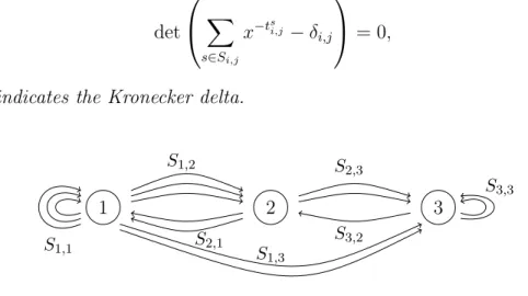
Theorem 2.2. Suppose the transmission is done by an automaton with d states, and from each state i any signal from a different group S_i,j can be transmitted with trans- mission time t^s_i,j, after which the automaton reaches state j, see Figure 11. Then the capacity of the channel is Cap= logλ where λ is the leading root of the equation

det



 X

s∈S_i,j

x^−tsi,j −δ_i,j



= 0, where δ_i,j indicates the Kronecker delta.

3 1

S_1,2

S2,1

2

S_2,3

S3,2

S1,1

S_3,3

S_1,3

Figure 11: A transmission automaton.

Proof. LetW_j(t) denote the number of possible signals of length tending at state j, so Wj(t) = X

i,s∈S_i,j

Wi(t−t^s_i,j). (4)

Use the ansatz W_j(t) =a_jx^t. Then (4) gives X

i,s∈S_i,j

ai x^−tsi,j −δi,j

for all j ≤d.

These equations can only have a simultaneous nontrivial solution (a₁, . . . , a_R) if

det



 X

s∈Si,j

x^−tsi,j −δ_i,j



= 0.

Therefore Cap = limt→∞ 1 t

Pd

j=1a_jx^t= logx.

It makes sense to expand this idea of transmission automaton to a Markov chain, where each transmission s ∈ S_i,j happens with a certain probability p^s_i,j such that PR

j=1

P

s∈Si,jp^s_i,j = 1 for every 1 ≤ i ≤ d. For example, if the states i ∈ A are the letters in the English alphabet, the transmissions are single letters j ∈ A and the probabilities p^j_i,j are the diagram frequencies of ij, conditioned to the first letter i.

Ergodicity is guaranteed if the graph of this automaton is strongly connected. Also, if π_j is the stationary probability of being in state j ∈ {1, . . . , d}, then

π_j =

d

X

i=1

π_i X

s∈S_i,j

p^s_i,j for all j ∈ {1, . . . , d}, see the Perron-Frobenius Theorem.

Shannon introduced an uncertainty function H =H(p₁, . . . , p_d) as a measure of the amount of uncertainty of the state we are in, if only the probabilities p₁, . . . , p_d of the events leading to this state are known. This function should satisfy the following rules:

1. H is continuous in all of its arguments;

2. If pi = ¹_d for all d ∈ N and i ∈ {1, . . . , d}, then d 7→ E(d) := H(¹_d, . . . , ¹_d) is increasing;

3. If the tree of events leading to the present state is broken up into subtrees, the uncertainty H is the weighted average of the uncertainties of the subtrees (see Figure 12):

H(p1, . . . , pd) =H(p1+p2, p3, . . . , pd) + (p1+p2)H(p,1−p).

•

•p1

•p2

•p3

...

... ...

• pd−1

•p_d

•

p₁+p₂•

•p

•1−p

•p3

...

... ...

• pd−1

•p_d Figure 12: Illustrating rule (3) of the uncertainty function.

Theorem 2.3. EFor every uncertainty function satisfying rules (1)-(3) is of the form

H(p₁, . . . , p_d) =−c

d

X

i=1

p_ilogp_i for some c≥0.

In particular,E(d) =clogdandH(p₁, . . . , p_d) = 0 ifp_i ∈ {0,1}for eachi. Assuming that the total number of transmission words is indeedd, then it is a natural to normalize, i.e., take c= 1/logd, or equivalently, to compute logarithms in base d.

Proof. If we break up an equal choice of d² possibilities into first d equal possibilities followed by d equal possibilities, we obtain

E(d²) := H(1

d², . . . , 1

d²) = H(1

d, . . . , 1 d) +

d

X

i=1

1 dH(1

d, . . . ,1

d) = 2E(d).

Induction gives E(d^r) = rE(d). Now choose 2 ≤ a, b ∈ N and r, s ∈ N such that a^r ≤ b^s < a^r+1. Taking logarithms gives ^r_s ≤ _log^log_a^b ≤ ^r+1_s . The monotonicity of rule (2) also gives

rE(a) =E(a^r)≤E(b^s) = sE(b),

so taking logarithms again, we obtain ^r_s ≤ _E(a)^E(b) ≤ ^r+1_s . Combining the two, we obtain

E(b)

E(a)− logb loga

≤ 2 s. Since s∈N can be taken arbitrarily large, it follows that

E(b) =clogb for c= E(a)

loga. (5)

The monotonicity of rule (2) implies thatc≥0.

Now assume that p_i = n_i/N for integers n_i and N = Pd

i=1n_i. By splitting the choice into N equal possibilities into d possibilities with probability p_i, each of which is split intoni equal possibilities, by (3), we get

E(N) = H(p₁, . . . , p_d) +

d

X

i=1

p_iE(n_i).

Inserting (5), we obtain H(p₁, . . . , p_d) =−c

d

X

i=1

p_i(logn_i−logN) = −c

d

X

i=1

p_ilog n_i N =−c

d

X

i=1

p_ilogp_i. This proves the theorem for all rational choices of (p1, . . . , pd). The continuity of rule (1) implies the result for all real probability vectors.

Suppose we compose messages of n symbols in {0,1}, and each symbol has proba- bility p₀ of being a 0 and p₁ = 1−p₀ of being a 1, independently of everything else.

Then the bulk of such messages has np₀ zeros and np₁ ones. The exponential growth rate of the number of such words is, by Stirling’s formula

n→∞lim 1 nlog

n np₀

= lim

n→∞

1

nlog nⁿe⁻ⁿ√

2πn (np₀)^np0e^−np0√

2πnp₀ (np₀)^np0e^−np0√ 2πnp₀

= −p₀logp₀ −p₁logp₁ =H(p₀, p₁).

Exercise 2.4. Show that you get the same result for the exponential growth rate if A={1, . . . , d} and the probability of transmitting a∈ A is p_a.

Recall the convenience of using logarithms base d if the alphabet A ={1,2, . . . , d}

hasdletters. In this base, the exponential growth rate isH(p₁, . . . , p_d)≤1 with equality if and only if all p_a = 1/d. Thus the number of the most common words (in the sense of the frequencies of a ∈ A deviating very little from p_a) is roughly d^{nH(p1,...,pd)}. This suggests that one could recode the bulk of the possible message with words of length nH(p₁, . . . , p_d) rather than n. Said differently, the bulk of the words x₁. . . x_n have measure

p(x₁, . . . x_n) =

n

Y

i=1

p_xi ≈e^{−nH(p1,...,pd)}.

By the Strong Law of Large Numbers, for all ε, δ >0 there is N ∈N such that for all n≥N, up to a set of measure ε, all wordsx₁. . . x_n satisfy

−1

nlog_dp(x₁. . . x_n)−H(p₁, . . . , p_d)

< δ.

Thus, suchδ-typical words can be recoded using at most n(H(p1, . . . , pd) +o(1)) letters for large n, and the compression rate is H(p₁, . . . , p_d) + o(1) as n → ∞. Stronger compression is impossible. This is the content of Shannon’s Source Coding Theorem:

Theorem 2.5. For a source code of entropy H and a channel with capacity Cap, it is possible, for any ε >0, to design an encoding such that the transmission rate satisfies

Cap

H −ε≤E(R)≤ Cap

H . (6)

No encoding achieves E(R)> ^Cap_H .

That is, for every ε >0 there is N₀ such that for very N ≥N₀, we can compress a message ofN letter with negligible loss of information into a message of N(H+ε) bits, but compressing it in fewer bit is impossible without loss of information.

Proof. Assume that the source messages are in alphabet{1, . . . , d}and letterss_iappear independently with probability p_i, so the entropy of the source is H = −P

ip_ilogp_i. For the upper bound, assume that the ith letter from the source alphabet require t_i bits to be transmitted.

The expected rate E(R) should be interpreted as the average number of bits that a bit of a “typical” source message requires to be transmitted. Let L_N be the collection ofN-letter words in the source, and µ_N be theN-fold Bernoulli product measures with probability vectorp= (p₁, . . . , p_d}. Let

AN,p,ε ={s∈ LN :||s|_i

N −pi|< ε for i= 1, . . . , d}.

By the Law of Large Numbers, for any δ, ε >0 there isN₀ such thatµ_N(A_N,p,ε)>1−δ for allN ≥N₀. This suggests that a source messagesbeing “typical” meanss ∈A_N,p,ε, and the transmission length of s is therefore approximately P

ip_it_iN. Thus typical words s ∈ L_N require approximately t = P

ip_it_iN bits transmission time, and the expected rate is E(R) = (P

ip_it_i)⁻¹.

For the capacity, the number of possible transmissions oft bits is at least the cardi- nality ofA_N,p,ε, which is the multinomial coefficient _p ^N

1N,...,pdN

. Therefore, by Stirling’s Formula,

Cap ≥ 1 t log

N p₁N, . . . , p_dN

≥ 1

P

ip_it_iN log (√

2πN)^1−d

d

Y

i=1

p^−(piN+

1 2) i

!

= −P

ip_ilogp_i P

ip_it_i − P

ilogp_i 2P

ip_it_iN +

d−1

2 log 2πN P

ip_it_iN ≥E(R)H, proving the upper bound (with equality in the limit N → ∞).

The coding achieving the lower bound in (6) that was used in Shannon’s proof resembled one designed by Fano [9]. It is now known as the Shannon-Fano code and works as follows:

For the lower bound, let again L_N be the collection of words B of length N in the source, occurring with probability p_B. The Shannon-McMillan-Breiman Theorem implies that for every ε >0 there is N₀ such that for all N ≥N₀,

| − 1

N logp_B−H|< ε for all B ∈ L_N except for a set of measure < ε.

Thus the average

G_N :=−1 N

X

B∈L_N

p_Blogp_B →H asN → ∞.

If we define the conditional entropy of symbola in the source alphabet following a word inL_N as

F_N+1 =H(Ba|B) =− X

B∈LN

X

a∈S

p_Balog₂ p_Ba p_B ,

then after rewriting the logarithms, we get (using telescoping series) FN+1 = (N + 1)G_N+1−N G_N, so G_N = _N¹ PN−1

n=0 F_n+1. The conditional entropy is decreasing as the words B get longer. Thus F_N is decreases in N and G_N is a decreasing sequence as well.

Assume that the words B₁, B₂, . . . , B_n ∈ L_N are arranged such that p_B1 ≥ p_B2 ≥

· · · ≥p_Bn. Shannon encodes the wordsB_i in binary as follows. LetP_s=P

i<sp_Bi, and choose m_s=d−logp_Bse, encodeB_s as the firstm_s digit of the binary expansion ofP_s, see Table 1. Because P_s+1 ≥P_s+ 2^−ms, the encoding of B_s+1 differs by at least one in the digits of the encoding of B_s. Therefore all codes are different.

The average number of bits per symbol isH⁰ = _N¹ P

sm_sp_Bs, so GN =−1

N X

s

pBslogpBs ≤H⁰ <−1 N

X

s

pBs(logpBs −1) =GN + 1 N. Therefore the average rate of transmission is

Cap H⁰ ∈

Cap

G_N +_N¹ , Cap G_N

.

Since G_N decreases to the entropy H, the above tends to Cap/H as required.

p_Bs P_s m_s Shannon Fano

8 36

28

36 3 110 11

7 36

21

36 3 101 101

6 36

21

36 3 011 100

5 36

15

36 3 010 011

4 36

6

36 4 0010 010

3 36

3

36 4 0001 001

2 36

1

36 5 00001 0001

1 36

0

36 6 00000(0) 0000

Table 1: An example of encoding using Shannon code and Fano code.

Fano [9] used a different and slightly more efficient encoding, but with the same effect (the difference negligible for large values of N). He divides L_N into two groups of mass as equal to 1/2 as possible. The first group gets first symbol 1 in its code, the other group 0. Next divide each group into two subgroups of mass as equal to 1/2×

probability of the group as possible. The first subgroups get second symbol 1, the other subgroup 0, etc. See Table 1.

2.2 Data Compression over Noisy Channels

Shannon’s Source Code Theorem 2.5 extends to noisy transmission channels, i.e., chan- nels through which a certain percentage of the transmissions arrive in damaged form.

The only thing to changed in the statement of the theorem is the definition of capacity.

For example, imagine a binary message, with symbol probabilities₀ andp₁ = 1−p₀, is transmitted and a fractionq of all the symbols is distorted from 0 to 1 and vice versa.

This means that symbol i in the received signal y has a chance

P=P(x=i|y=i) = p_i(1−q) + (1−p_i)q

0 0

q

1 1

q 1−q

1−q

(7)

in the sent signalx. Ifq= ¹₂, thenP= ¹₂, so every bit of information will be transmitted with total unreliability. But also if q is small, P can be very different from P(y = i).

For example, if p₀ = q = 0.1, then P = 0.1(1−0.01) + (1−0.1)0.1 = 0.18. The key notion to measure this uncertainty of sent symbol is the conditional entropy of x given that y is received:

H(x|y) = −X

i,j

P(x_i∧y_j) log P(x_i∧y_j) P(y_j)

were the sum is over all possible sent message x_i and received messages y_j. This uncertainty H(x|y) is called the equivocation. If there is no noise, then knowing y gives full certainty about x, so the equivocation H(x|y) = 0, but also q= 1, i.e., every symbol is received distorted, knowing y gives full knowledge of x and H(x|y) = 0. In the above example:

H(x|y) = −p₀(1−q) log₂ p₀(1−q)

p₀(1−q) +p₁q −p₁qlog₂ p₀q p₀(1−q) +p₁q

−p₁(1−q) log₂ p₁(1−q)

p0q+p1(1−q)−p₀qlog₂ p₀q

p0q+p1(1−q). (8) The actual information transmitted, known as themutual information, is defined as

I(X|Y) = H(x)−H(x|y)

In, say, the binary alphabet, we can interpret 2^H(x)n+o(n) as the approximate possible number of length n source messages, up to a set of measure ε, that tends to with an error that tends to zero as n → ∞. For each source message x, the number of received messages y generated from x via transmission errors is 2^H(y|x)n+o(n), see Figure 13.

Analogous interpretations hold for 2^H(y)n+o(n) and 2^H(x|y)n+o(n).

The total number of non-negligible edges in Figure 13 is therefore approximately 2^H(x)n+o(n)·2H(y|x)n+o(n)≈2^H(y)n+o(n)·2H(x|y)n+o(n)≈2H(x∨y)n+o(n)

.

Taking logarithms, dividing by−n, taking the limitn → ∞and finally adding H(x) + H(y) gives the helpful relations

I(X|Y) =H(x)−H(x|y) =H(y)−H(y|x) =H(x) +H(y)−H(x∨y). (9) If the noiseless channel capacity Cap_noiseless is less than the equivocation, then it is impossible to transmit the message with any reliable information retained. Simply, uncertainty is produced faster than the channel can transmit. If the equivocation is less than the capacity, then by adding (otherwise superfluous) duplicates of the message, or control symbols, the message can be transmitted such that it can be reconstructed afterwards if negligible errors. However, the smaller the difference Cap_noiseless−H(x|y),































2^H(x)nhigh probability

messages































2^H(y)nhigh probability received signals

••

••

••

••

••

••

••

••

••

••

••

••

••

••

••

••

••

•

2^H(x|y)nhigh probability causes fory

2^H(y|x)nhigh probability effects ofx

Figure 13: Interpreting 2^H(x)n, 2^H(y)n, 2^H(x|y)n and 2^H(y|x)n

the more duplicates and/or control symbols have to be send to allow for reconstruction.

It turns out that the correct way to define the capacity of a noisy channel is Cap_noisy= max

x I(X|Y) = max

x H(x)−H(x|y)

where the maximum is taken over all possible source messages only, because the distri- bution of the received messages can be derived from x and knowledge to what extent the channel distorts messages. The distribution of x that achieves the maximum is called theoptimal input distribution. To compute Cap_noisy in the example of (8) we need to maximize H(x)−H(x|y) over p₀ (because p₁ = 1−p₀ and q is fixed). Due to symmetry, the maximum is achieved atp= ¹₂, and we get

Cap_noisy = log₂2 +qlog₂q+ (1−q) log₂(1−q). (10)

This confirms full capacity 1 = log₂2 if there is no noise and Cap_noisy= 0 if q= ¹₂. Let Q = (q_ij) be the probability matrix where q_ij stands for the probabiity that symbol i ∈ S is received as j ∈ A. Thus if S = A, then qii is the probability that symbol i is transmitted correctly.

Proposition 2.6. Assuming that Q is an invertible square matrix with inverse Q⁻¹ = (q⁻¹_ij ), the optimal probability for this noisy channel is

p_i =X

t

q_ti⁻¹exp −Cap_noisyX

s

q⁻¹_ts +X

s,j

q⁻¹_ts q_sjlogq_sj

! ,

where the noisy capasity Cap_noisy should be chosen such that P

ip_i = 1.

Proof. We maximize

I(X|Y) = −X

i

pilogpi+X

i,j

piqijlog piqij

P

kp_kq_kj

= X

i,j

p_iq_ijlogq_ij−X

i,j

p_iq_ijlogX

k

p_kq_kj

over p_i subject to P

ip_i = 1 using Lagrange multipliers. This gives X

j

q_sjlog q_sj P

kp_kq_kj =µ for all s∈ S. (11) Multiply the equations (11) with p_s (with P

sp_s= 1) and sum over s to get µ=X

s,j

p_sq_sjlog q_sj P

kpkqkj

= Cap_noisy.

Now multiply (11) with q_ts⁻¹, sum overs and take the exponential. This gives X

k

p_kq_kt= exp X

s,j

q_ts⁻¹q_sjlogq_sj −Cap_noisyX

s

q_ts⁻¹

! .

Therefore

p_i =X

t

q⁻¹_ti exp X

s,j

q_ts⁻¹q_sjlogq_sj −Cap_noisyX

s

q_ts⁻¹

! ,

as claimed.

Remark 2.7. Suppose that the matrix Q has a diagonal block structure, i.e., the source alphabet can be divided into groups g with symbols in separate groups never mistaken for one another. Then Cap_noisy = log₂P

g2^Capg, where Cap_g is the noisy ca- pacity of the group g. The optimal probability for all symbols in group g together is P^g = 2^Capg/P

g⁰2^Capg0.

Exercise 2.8. The noisy typewriter is a transmission channel for the alphabet{a, b, c, . . . , z,−}, where − stands for the space. Imagine a circular keyboard on which typing a letter re-

sults in that latter or to one of its neighbors, all three with probability 1/3.

1. Compute the capacity Cap_noisy of this channel and an optimal input distribution.

2. Find an optimal input distribution so that the received message can be decoded without errors.

Going back to Figure 13, assume that among the most likely transmissions, we choose a maximal subcollection that have disjoint sets of most likely received messages.

The cardinality of this subcollection is approximately 2^H(y)n

2^H(y|x)n = 2(H(y)−H(y|x))n ≤2^nCapnoisy.

Then such received messages can be decoded with a negligible amount of error. Maxi- mizing over all input distributions, we obtain that a message can be transmitted virtu- ally error-free at a rate of C bits per transmitted bit. This is a heuristic argument for Shannon’s Noisy Source Code Theorem.

Theorem 2.9. For transmission of a message of entropy H through a noisy channel with capacity Cap_noisy and any ε >0, there is N0 ∈N such that every message of length N ≥ N₀ can be transmitted through the channel at expected rate E(R) arbitrarily close to ^Cap_H^noisy such that the proportion of errors is at most ε.

If we allow a proportion of errors δ, the expected rate for this proportion of errors is E(R(δ)) can be made arbitrarily close to _H(1−h^Capnoisy

2(δ)), for the entropy functionh₂(δ) =

−δlog₂δ−(1−δ) log₂(1−δ). Faster rates at this proportion of errors cannot be achieved.

Proof. We will give the proof for the binary channel of (7), so the channel capacity is Cap_noisy = 1 +qlog₂q+ (1−q) log₂(1−q) =: 1−h₂(q) as in (10). This gives no loss of generality, because we can always recode the source (of entropy H) into binary in an entropy preserving way³. By the Noiseless Source Code Theorem 2.9, the rate “gains” a factor 1/H because the compression from the source alphabet into the binary alphabet occurs at a noiseless capacity Cap = lim_t¹_tlog 2^t = 1. This factor we have to multiply the rate with at the end of the proof.

Also we will use linear codes such as Hamming codes⁴ which postdate Shannon’s proof, but shows that already an elementary linear code suffices to achieve the claim of the theorem.

Assume that the source messages have length K, which we enlarge by M parity check symbols to a source code x of length N = K+M. This is done by a Hamming code in the form of an M×N matrix L∈F^M2 ^×N of which the rightM ×M submatrix is the parity check matrix. When x is transmitted over the noisy binary channel, approximately N q errors appear, i.e., N q symbols are flipped, and the received word is y = x+w, where w stands for the noise. It is a sample of N Bernoulli trials with success (i.e., error) chance q, occurring with probability q^|w|1(1−q)^|w|0.

For an arbitrary ε >0, there is some constant C_ε such that the noise wordsw with

|w|₁ >(N+C_ε√

N)q have total probability < ε/2. The number of noise wordsw with

|w|₁ ≤(N +C√

N)q is ≤2^(N+Cε

√

N)h2(q).

The choice of a Hamming code defines the actual transmission, so we can decide to choose x according to the optimal input distribution. This will give an output distribution satisfyingH(y)−H(y|x) = Cap_noisy, and we can select a subset of “typical”

outcomes Ytyp as those produce from some source x and a non-typical noise w. The probability of not being in Ytyp is less than ε/2.

There are altogether 2^M syndromes, i.e., outcomes of S(y) = yL^T ∈ {0,1}^M. The Hamming encoding satisfiesS(x) = 0, soS(y) = S(x+w) =S(w). The sets {y∈Ytyp:

3Note that we may have to use blocks of 0s and 1s instead of single symbols if the entropy is larger than log 2.

4For this proof we would like to acknowledge the online lectures by Jacob Foerster (Cambridge University) https://www.youtube.com/watch?v=KSV8KnF38bs, based in turn on the text book [18].

S(y) = z} are the 2^M disjoint subsets of Ytyp from which x can be reconstructed, by subtracting the coset leader of S(y) from y. This is error-free except (possibly) if

1. y /∈Ytyp, but this happens with probability ≤ε/2, independently of the choice of Hamming encoding;

2. there is some other ˜y= ˜x+ ˜w∈Ytyp such that S(˜y) =S(y), i.e., S( ˜w−w) = 0.

The probability that the latter happens X

y=x+w∈Ytyp

P(w)1_{{∃ w6=w˜ ˜y∈Ytyp( ˜w−w)L}^T_=0} ≤X

w

P(w)X

w6=w˜

1_{{( ˜w−w)L}^T_=0}.

is difficult to compute. However, we can average over all 2^M2 possible M×N-matrices L, occurring with probability P(L). This gives an average failure probability less than

X

L

P(L)X

w

P(w)X

˜ w6=w

1_{{( ˜w−w)L}^T_=0} ≤X

w

P(w)X

˜ w6=w

X

L

P(L)1_{{( ˜w−w)L}^T_=0}.

The inner sum, however, equals 2^−M because the probability of any entry of ( ˜w−w)L^T being zero is 1/2, independent of all other entries. Since there are 2^(N+Cε

√

N)h2(q)possible noises ˜w such that ˜y ∈ Ytyp, the average failure probability over all Hamming codes is

≤ 2^(N+Cε

√N)h2(q)2^−M. Assuming that N(h₂(q) + 2ε) > M ≥ N(h₂(q) + ε) > N, this probability is ≤ 2^{−N ε} < ε/2. Therefore the failure probability averaged over all Hamming codes is at mostε, and therefore there must exist at least one (probably many) Hamming code that achieves the required failure rate. Buth₂(q)+2ε > M/N ≥h₂(q)+ε implies that the transmission rate for this Hamming code satisfies

Cap_noisy−2ε < K

N = 1− M

N = 1−h₂(q)−ε ≤Cap_noisy−ε, as claimed.

For the second statement, that is, if we allow a proportion δ of errors, we use the Hamming code of the first part of the proof in reverse. We chop the source message into blocks of lengthN and consider each block as a code word of which the lastM bits play the role of parity check symbols (although they really aren’t) and the first K bits play the role of actual information. For typical messages (i.e., all up to an error εof all the possible blocks inL_N), we can use a Hamming code for which M =dh₂(δ)Ne, and then we throw these symbols simply away. We choose the initial block size N that he remainingK =N−M =N(1−h2(δ)) bits are at the capacity of the noisy channel, i.e., these K bits take Cap_noisyK bits to transmit, virtually error-free. But then a typical originalN bits message takes ^Cap_1−h^noisy

2(δ)N bits to transmit at an error proportionδ, so the expected noisy rate E(R(δ)) = ^Cap_1−h^noisy

2(δ), proving the second part.

Let us now argue that the rateRcannot exceed the capacity Cap_noisy, following [22].

We will use a code ofn-letter code words on a two-letter alphabet; the loss of generality

in this choice becomes negligible as nto∞. There are thus 2^nR code words among 2ⁿ n-letter words in total, and for this rate th code is optimally used if all the code words have probability 2^−nR of occurring, and hence the entropy of code words Xⁿ chosen according uniform distribution is H(Xⁿ) = nR. The received message Yⁿ is also an n-letter word, and since Xⁿ is sent letter by letter, with errors occurring independently in each letter,

P(Yⁿ|Xⁿ) = P(y1y2. . . yn|x1x2. . . xn) =

n

Y

i=1

P(yi|xi).

Hence the conditional entropy, being the average of minus the logarithm of the above quantity, satisfies

H(Yⁿ|Xⁿ) = −

n

X

i=1

P(y_i|x_i) logP(y_i|x_i) =

n

X

i=1

H(uy_i|x_i).

Entropy is subadditive, so the mutual information is I(Yⁿ|Xⁿ) =H(Yⁿ)−H(Yⁿ|Xⁿ)≤

n

X

i−=1

H(y_i)−H(y_i|x_i) =

n

X

i=1

I(y_i|x_i)≤nCap_noisy, (12) because Cap_noisy is the mutual information maximized over all input distributions. By the symmetry of (9), also

I(Yⁿ|Xⁿ) =H(Xⁿ)−H(Xⁿ|Yⁿ) =nR−H(Xⁿ|Yⁿ) =

n

X

i=1

I(yi|xi)≤nCap_noisy, (13) Reliably decoding the received message means that ¹_nH(Xⁿ|Yⁿ) → 0 as n → ∞.

Hence, combining (13) and (12) gives R ≤ Cap_noisy+o(1) as n → ∞. This gives the upper boundR ≤Cap_noisy.

2.3 Symbol Codes

Shannon’s Source Code Theorem 2.5 gives the theoretical optimal bounds for encoding messages in the shortest way. Suppose that a source S is an ensemble from which the elements s ∈ S are produced with frequencies p_s, so the source entropy is H(S) = P

s∈Sp_slogp_s. Translating Shannon’s Theorem, assuming that the channel is simple such that the capacity is log_dd = 1, for every ε > 0 there exists a code that turns a string s₁. . . s_n of sampled symbols such into a code word c(s₁. . . s_n) where

nH(S)≤ |c(s₁. . . s_n)| ≤n(H(S) +ε) asn → ∞, (14) and no code performs better (without losing information) thatnH(S). What are prac- tical codes that achieve this? That is, an code c that:

1. turns every string s₁. . . s_n from the source into a string a₁. . . a_k in the code alphabet A;

2. is uniquely decodable (or lossless, i.e., can be inverted;

3. achieves (14) with ε as small as possible;

4. is easily computable, i.e., cheap, quick and preferably without the use of a huge memory.

The first thing to try is a symbol code, i.e, c assigns a string c(s) ∈ A^∗ of to each s ∈ S, and extend this by concatenation. That is, a symbol code is a substitution, except that it is not necessarily stationary. The rule encode si in the source string is allowed to depend on the context, or rather the history si−1, si−2, . . .

Definition 2.10. A prefix (suffix) code is a code csuch that no code word c(s) is a prefix (suffix) of any other code words c(s⁰).

It is easy to verify that Shannon code and Fano code are both prefix (but not suffix) codes.

Lemma 2.11. Every prefix and suffix code is uniquely decodable.

Proof. Suppose c is a prefix code and c(s₁. . . s_n) = a₁. . . a_k. Start parsing from the left, until you find the first a₁. . . a_j =c(s) for some s ∈ S. Since c(s) is not the prefix of any other c(s⁰), we must have s =s₁. Continue parsing from symbol a_j+1, etc. For suffix codes we do the same, only parsing from right to left.

Since it is uncommon to parse from right to left (in the direction messages are transmitted), we always prefer prefix codes over suffix codes. In this, decodable is different from the notion recognizable in substitution shift, because decoding algorithms cannot depend on future digits. Any prefix code can be represented as an edge-labeled subtree of the binary tree (or d-adic tree if d = #A) in which each code word is the label of a path from the root to a leaf (i.e, a non-root vertex that has only one edge connected to it), see Figure 14.

The following condition, called the Kraft inequality, is a necessary condition for a symbol code to be uniquely decodable.

Proposition 2.12. A uniquely decodable code with codewords c(s) in alphabet A with d= #A satisfies

X

s∈S

d^−|c(s)|≤1, (15)

Proof. Let d = #A and `<sub>s</sub> = |c(s)|, so 1 ≤ `_s ≤ `<sub>max</sub> for the maximum code word length `_max. Let K =P

sd^−`s, and therefore

Kⁿ = X

s

d^−`s

!n

=

`max

X

s1=1

· · ·

`max

X

sn=1

d^{−(`s1+···+`sn)}

•

• •

• •

• • •

• •

root

0 1

0 1

0 1 1

0 1

Used codewords:

0 100 101 1110 1111

Figure 14: An example of a tree representing prefix code.

But each word is uniquely decodable, so to every string xof length ` ≤n`_max, there is at most one choice of s₁, . . . , s_n such thatx=c(s₁). . . c(s_n). Since there at at most n^` words of this length, we get

Kⁿ≤

n`max

X

`=n

d^{`</sup>d<sup>−`} ≤n`_max.

Taking the n-th root on both sides and th limit n→ ∞, we get K ≤1.

If equality holds in (15), then we say that the code is complete. For a complete code, the average frequencies of eacha ∈ Amust be 1/d(and there cannot be correlation between digits), because otherwise the entropy of the encoding is not maximal and we could encode it further.

Prefix/suffix codes that fill the subtree entirely are complete. Indeed, such a code has d−1 words of length k and d words of the maximal length n, so

X

s

d^−c(s)≤(d−1)

n−1

X

k=1

d^−k+d·d⁻ⁿ = 1.

Every unique decodable code c is equivalent to a prefix code. To see this, order s ∈ S according to their code word lengths, and then recode them lexicographically, main- taining code length, and avoiding prefixes. Due to the Kraft inequality, there is always space for this.

For the next result, we need the Gibbs inequality

Lemma 2.13. If (p_s) and (q_s) are probability vectors, then the Gibbs inequality

Xp_slog_dp_s/q_s ≥0 (16) holds with equality only if q_s =p_s for all s.