V.M. Braun, a A.N. Manashov, b,a S. Moch b and M. Strohmaier a

JHEP06(2017)037

Published for SISSA by Springer

Received : March 30, 2017 Accepted : May 28, 2017 Published : June 7, 2017

Three-loop evolution equation for flavor-nonsinglet operators in off-forward kinematics

V.M. Braun, ^a A.N. Manashov, ^b,a S. Moch ^b and M. Strohmaier ^a

a Institut f¨ ur Theoretische Physik, Universit¨ at Regensburg, D-93040 Regensburg, Germany

b Institut f¨ ur Theoretische Physik, Universit¨ at Hamburg, D-22761 Hamburg, Germany

E-mail: vladimir.braun@physik.uni-regensburg.de, alexander.manashov@desy.de, sven-olaf.moch@desy.de, matthias.strohmaier@ur.de

Abstract: Using the approach based on conformal symmetry we calculate the three- loop (NNLO) contribution to the evolution equation for flavor-nonsinglet leading twist operators in the MS scheme. The explicit expression for the three-loop kernel is derived for the corresponding light-ray operator in coordinate space. The expansion in local operators is performed and explicit results are given for the matrix of the anomalous dimensions for the operators up to seven covariant derivatives. The results are directly applicable to the renormalization of the pion light-cone distribution amplitude and flavor-nonsinglet generalized parton distributions.

Keywords: Perturbative QCD, Renormalization Group

ArXiv ePrint: 1703.09532

JHEP06(2017)037

Contents

1 Introduction 1

2 Evolution equations for light-ray operators 3

3 Similarity transformation 7

4 Reciprocity relation 10

5 Three-loop invariant kernel H ⁽³⁾ _inv 12

5.1 Splitting functions 14

5.2 Mellin transformation 16

6 From light-ray to local operators 20

7 Conclusions 27

A Two-loop invariant kernel 28

B X kernels 28

C T kernels 31

1 Introduction

The remarkable progress in experimental techniques in the past two decades has provided a fresh impetus to the study of hard exclusive and semi-inclusive reactions with identified particles in the final state. Such processes are interesting as they allow one to access the hadron structure on a much more detailed level as compared to totally inclusive reactions.

A (probably still distant) major goal is to understand the full three-dimensional proton structure by “holographic imaging” of quark and gluon distributions in transverse distance and momentum spaces. The related experiments have become a prominent part of the research program at all major existing and planned accelerator facilities, e.g. the Electron Ion Collider (EIC) [1].

The relevant nonperturbative input in such processes in many cases involves operator

matrix elements between states with different momenta, dubbed generalized parton distri-

butions (GPDs), or vacuum-to-hadron matrix elements related to light-front hadron wave

functions at small trans- verse separations, the distribution amplitudes (DAs). The scale-

dependence of such distributions is governed by the renormalization group (RG) equations

for the corresponding operators, where, in contrast to standard parton densities, mixing

with the operators involving total derivatives has to be taken into account. Going over to

JHEP06(2017)037

local operators one has to deal with a triangular mixing matrix where the diagonal entries are the anomalous dimensions, the same as in deep-inelastic scattering, but the off-diagonal elements require a separate calculation.

The projected very high accuracy of future experimental data, e.g. on the Deeply Virtual Compton Scattering (DVCS) at the JLAB 12 GeV upgrade [2] and the EIC, and the γ ^∗ → πγ transition form factor at Belle II at KEK [3], has to be matched by the increasing theoretical precision; in the ideal case one would like to reach the same level of accuracy as in inclusive reactions. The NNLO (three-loop) analysis of parton distributions and fragmentation functions is becoming the standard in this field [4], so that the NNLO evolution equations for off-forward distributions are appearing on the agenda.

In this work we derive the explicit expression for the three-loop contribution to the flavor-nonsinglet evolution kernel in the so-called light-ray operator representation. This kernel can be converted to the evolution equation for the GPDs by a Fourier transformation, whereas its expansion at small distances provides one with the matrix of the anomalous dimensions for local leading twist operators. In the latter form, our results are directly relevant for the lattice calculations of pion DAs in which case the uncertainty due to the conversion of lattice results to the MS scheme currently proves to be one of the dominant sources of the error [5]. The three-loop (NNLO) anomalous dimensions of the leading-twist operators are known for about a decade [6], however, a direct calculation of the missing off-diagonal terms in the mixing matrix to the same precision is quite challenging.

Conformal symmetry of the QCD Lagrangian allows one to restore the nondiagonal entries in the mixing matrix and, hence, full evolution kernels at a given order of perturba- tion theory from the calculation of the special conformal anomaly at one order less [7]. This result was used to calculate the complete two-loop mixing matrix for twist-two operators in QCD [8–10], and to derive the two-loop evolution kernels for the GPDs [11–13].

In ref. [14] we have proposed to use a somewhat different technique to implement the same idea. Instead of studying conformal symmetry breaking in the physical theory [8–10]

we suggest to make use of the exact conformal symmetry of large-n _f QCD in d = 4 − 2 dimensions at critical coupling. Due to specifics of the minimal subtraction scheme (MS) the renormalization group equations in the physical four-dimensional theory inherit a con- formal symmetry so that the evolution kernel commutes with the generators of conformal transformations. This symmetry is exact, however, the generators are modified by quan- tum corrections and differ from their canonical form. The consistency relations that follow from the conformal algebra can be used in order to restore the `-loop off-forward kernel from the `-loop anomalous dimensions and the (` − 1)-loop result for the deformation of the generators, which is equivalent to the statement in ref. [7].

Exact conformal symmetry of modified QCD allows one to use algebraic group-theory

methods to resolve the constraints on the operator mixing and also suggests the optimal

representation for the results in terms of light-ray operators. In this way one avoids the

need to restore the evolution kernels from the results for local operators, which is not

straightforward. This modified approach was tested in [14] on several examples to two-

and three-loop accuracy for scalar theories, and in [15] for flavor-nonsinglet operators in

QCD to two-loop accuracy. As a major step towards the NNLO calculation, in [16] we have

JHEP06(2017)037

calculated the two-loop quantum correction to the generator of special conformal trans- formations. In this work we use this result to obtain the three-loop (NNLO) evolution equation for flavor-nonsinglet leading twist operators in the light-ray operator representa- tion in the MS scheme. The relation to the representation in terms of local operators [7–9]

is worked out in detail and explicit results are given for the matrix of the anomalous di- mensions for the operators with up to seven covariant derivatives. Our results are directly applicable e.g. to the studies of the pion light-cone DA and flavor-nonsinglet GPDs.

The presentation is organized as follows. Section 2 is introductory, it contains a very short general description of the light-ray operator formalism and the conformal algebra.

In this section we also explain our notation and conventions. In section 3 we show that the contributions to the evolution kernel due to the conformal anomaly can be isolated by a similarity transformation. As the result, the evolution kernel can be written as a sum of several contributions with a simpler structure. This construction is similar in spirit to the “conformal scheme” of refs. [8–10]. We find that the remaining (canonically) SL(2)- invariant part of the three-loop kernel satisfies the reciprocity relation [17–20], discussed in section 4. The explicit construction of the invariant kernel is presented in section 5.

We provide analytic expressions for the terms that correspond to the leading asymptotic behavior at small and large Bjorken x, and a simple parametrization for the remainder that has sufficient accuracy for all potential applications. In section 6 we explain how our results for the renormalization of light-ray operators can be translated into anomalous dimension matrices for local operators. In this way also the formal relation to the results in [7–9] is established. The final section 7 is reserved for a summary and outlook. The paper also contains several appendices where we collect the analytic expressions for the kernels.

2 Evolution equations for light-ray operators

A renormalized light-ray operator,

[O](x; z ₁ , z ₂ ) = ZO(x; z ₁ , z ₂ ) = Z q(x ¯ + z ₁ n)/ nq(x + z ₂ n), (2.1) where the Wilson line is implied between the quark fields on the light-cone, is defined as the generating function for renormalized local operators:

[O](x; z ₁ , z ₂ ) ≡ X

m,k

z ₁ ^m z ₂ ^k m!k!

h

¯

q(x)( D ^← ·n) ^m n(n· / D ^→ ) ^k q(x) i

, (2.2)

where D _µ = ∂ _µ − igA _µ is the covariant derivative. Here and below we use square brackets to denote renormalized composite operators (in a minimal subtraction scheme). Due to Poincare invariance in most situations one can put x = 0 without loss of generality; we will therefore often drop the x dependence and write

O(z ₁ , z ₂ ) ≡ O(0; z ₁ , z ₂ ).

JHEP06(2017)037

The renormalization factor Z is an integral operator in z ₁ , z ₂ which is given by a series in 1/, d = 4 − 2,

Z = 1 +

∞

X

k=0

1

^k Z _k (a) , Z _k (a) =

∞

X

`=k

a ^{`</sup> Z <sub>k</sub> <sup>(`)} . (2.3) The RG equation for the light-ray operator [O] takes the form

M ∂ _M + β(a)∂ _a + H (a)

[O](x; z ₁ , z ₂ ) = 0 , (2.4) where M is the renormalization scale,

a = α s

4π , β(a) = M da

dM = −2a + aβ 0 + a ² β 1 + . . .

= −2a( + ¯ β(a)) (2.5) with

β ₀ = 11

3 N _c − 2

3 n _f , β ₁ = 2 3

17C _A ² − 5C _A n _f − 3C _F n _f

. (2.6)

H (a) is an integral operator acting on the light-cone coordinates of the fields, which has a perturbative expansion

H (a) = a H ⁽¹⁾ + a ² H ⁽²⁾ + a ³ H ⁽³⁾ + . . . (2.7) It is related to the renormalization factor (2.3) as follows

H (a) = −M d

dM ZZ ⁻¹ = 2γ _q (a) + 2

∞

X

`=1

` a <sup>`</sup> Z ₁ ^(`) , (2.8) where Z = ZZ _q ⁻² ; Z q is the quark wave function renormalization factor and γ q = M ∂ M ln Z q

the quark anomalous dimension. The QCD β-function β(a) and γ _q are known to O(a ⁵ ) [21–25].

The evolution operator can be written as [26]

H (a)[O](z ₁ , z ₂ ) = Z 1

0

dα Z 1

0

dβ h(α, β) [O](z ₁₂ ^α , z ^β ₂₁ ) , (2.9) where

z ₁₂ ^α = z ₁ α ¯ + z ₂ α α ¯ = 1 − α , (2.10) and h(α, β) = a h ⁽¹⁾ (α, β)+a ² h ⁽²⁾ (α, β)+ . . . is a certain weight function (evolution kernel).

It is easy to see [14] that translation-invariant polynomials (z 1 −z ₂ ) ^N are eigenfunctions of the evolution kernel,

H (a)z ₁₂ ^N = γ N (a) z ₁₂ ^N z 12 = z 1 − z 2 . (2.11) The eigenvalues γ N (a) correspond to moments of the evolution kernel in the representa- tion (2.9),

γ _N = Z 1

0

dα Z 1

0

dβ (1 − α − β) ^N h(α, β) = aγ ⁽¹⁾ _N + a ² γ _N ⁽²⁾ + a ³ γ _N ⁽³⁾ + . . . . (2.12)

JHEP06(2017)037

They define the anomalous dimensions of leading-twist local operators in eq. (2.2) where N = m + k is the total number of covariant derivatives acting either on the quark or the antiquark field. The corresponding mixing matrix in the Gegenbauer polynomial basis is constructed in section 6.

The leading-order (LO) result for the evolution kernel in this representation reads [26]:

H ⁽¹⁾ f (z 1 , z 2 ) = 4C F

Z 1 0

dα α ¯ α h

2f (z 1 , z 2 ) − f (z ^α ₁₂ , z 2 ) − f(z 1 , z ₂₁ ^α ) i

− Z 1

0

dα Z α ¯

0

dβ f (z ^α ₁₂ , z ₂₁ ^β ) + 1

2 f(z ₁ , z ₂ )

. (2.13)

The expression in eq. (2.13) gives rise to all classical leading-order (LO) QCD evolution equations: the DGLAP equation for parton distributions, the ERBL equation for the meson light-cone DAs, and the general evolution equation for GPDs.

The LO evolution kernel H ⁽¹⁾ commutes with the (canonical) generators of collinear conformal transformations

S ₋ ⁽⁰⁾ = −∂ _z

− ∂ z

, S ₀ ⁽⁰⁾ = z 1 ∂ z

+ z 2 ∂ z

+ 2,

S ₊ ⁽⁰⁾ = z ₁ ² ∂ _z

+ z ₂ ² ∂ _z

+ 2(z ₁ + z ₂ ) (2.14) which satisfy the usual SL(2) algebra

[S ₀ , S ± ] = ±S _± , [S ₊ , S − ] = 2S ₀ . (2.15) It can be shown that as a consequence of the commutation relations [ H ⁽¹⁾ , S _α ⁽⁰⁾ ] = 0 the corresponding kernel h ⁽¹⁾ (α, β) is effectively a function of one variable τ called the conformal ratio [27]

h ⁽¹⁾ (α, β) = ¯ h(τ ) , τ = αβ

¯

α β ¯ , (2.16)

up to trivial terms ∼ δ(α)δ(β) that correspond to the unit operator. This function can easily be reconstructed from its moments (2.12), alias from the anomalous dimensions.

Indeed, it is easy to verify that the result in eq. (2.13) can be written in the following, remarkably simple form [27]

h ⁽¹⁾ (α, β) = −4C _F

δ + (τ ) + θ(1 − τ ) − 1

2 δ(α)δ(β )

, (2.17)

where the regularized δ-function, δ ₊ (τ ), is defined as Z

dαdβ δ ₊ (τ )f(z ₁₂ ^α , z ^β ₂₁ ) ≡ Z 1

0

dα Z 1

0

dβ δ(τ ) h

f (z ₁₂ ^α , z ₂₁ ^β ) − f (z ₁ , z ₂ ) i

= − Z 1

0

dα α ¯ α h

2f (z ₁ , z ₂ ) − f (z ₁₂ ^α , z ₂ ) − f (z ₁ , z ^α ₂₁ ) i

. (2.18)

Beyond the LO this property is lost. However, the evolution kernels for leading twist

operators in minimal subtraction schemes retain exact conformal symmetry. Indeed, the

JHEP06(2017)037

renormalization factors for composite operators in this scheme do not depend on by con- struction. As a consequence, the anomalous dimension matrices in QCD in four dimensions are exactly the same as in QCD in d = 4 − 2 dimensions that enjoys conformal symmetry for the specially chosen “critical” value of the coupling [14–16]. The precise statement is that the QCD evolution kernel H (a) commutes with three operators

[ H (a), S ₊ ] = [ H (a), S − ] = [ H (a), S ₀ ] = 0 (2.19) that satisfy the SL(2) algebra (2.15). These operators can be constructed as the generators of collinear conformal transformations in the 4 − 2-dimensional QCD at the critical point and have the following structure [14–16]:

S − = S ₋ ⁽⁰⁾ , (2.20a)

S ₀ = S ₀ ⁽⁰⁾ + ∆S ₀ = S ₀ ⁽⁰⁾ +

β(a) + ¯ 1 2 H (a)

, (2.20b)

S + = S ₊ ⁽⁰⁾ + ∆S + = S ₊ ⁽⁰⁾ + (z 1 + z 2 )

β(a) + ¯ 1 2 H (a)

+ (z 1 − z 2 ) ∆(a) , (2.20c) where ¯ β(a) is the QCD β -function (2.5) and S α ⁽⁰⁾ are the canonical generators (2.14).

Note that the generator S − corresponds to translations along the light cone and does not receive any corrections as compared to its canonical expression, S ₋ ⁽⁰⁾ . The generator S 0

corresponds to dilatations; its modification in interacting theory ∆S ₀ = S ₀ − S ₀ ⁽⁰⁾ can be related to the evolution kernel H(a) from general considerations [14]. Finally S + is the gen- erator of special conformal transformations and eq. (2.20c) is the most general expression consistent with the commutation relations (2.15). To see that, note that ∆S ₊ = S ₊ − S ₊ ⁽⁰⁾ must have the same canonical dimension [mass] ⁻¹ as S ⁽⁰⁾ ₊ , meaning that [S ₀ ⁽⁰⁾ , ∆S + ] = ∆S + . Thus we can write ∆S + = (z 1 + z 2 )∆ 1 + (z 1 − z 2 )∆ 2 where [S ₀ ⁽⁰⁾ , ∆ 1,2 ] = 0. Plugging this expression in the commutation relation [S + , S − ] = 2S 0 one obtains ∆ 1 = ∆S 0 and [S − , ∆ ₂ ] = 0. Changing notation ∆ ₂ 7→ ∆ we arrive at the expression given in eq. (2.20c).

Using (2.20) in the commutation relation [S ₀ , S ₊ ] = S ₊ , or equivalently [ H (a), S ₊ ] = 0, results in

S ₊ ⁽⁰⁾ , H (a)

= −

∆S + , H (a)

=

H (a), z 1 +z 2

β(a)+ ¯ 1 2 H (a)

+

H (a), z 12 ∆(a)

. (2.21) If H (a) is known, this equation can be used to find ∆(a) and in this way construct the SL(2) generators that commute with the evolution kernel in a theory with broken conformal symmetry. The main point is, however, that ∆(a) can be calculated independently from the analysis of the conformal Ward identity [7, 13, 16]. In this way eq. (2.21) can be used to calculate the non-invariant part of the evolution kernel with respect to the canonical generators S _±,0 ⁽⁰⁾ .

Indeed, expanding the kernels in a power series in coupling constant

H(a) = aH ⁽¹⁾ + a ² H ⁽²⁾ + a ³ H ⁽³⁾ + . . . , ∆(a) = a∆ ⁽¹⁾ + a ² ∆ ⁽²⁾ + . . . (2.22)

JHEP06(2017)037

one obtains from (2.21) a nested set of equations [14]

[S ₊ ⁽⁰⁾ , H ⁽¹⁾ ] = 0 , (2.23a)

[S ₊ ⁽⁰⁾ , H ⁽²⁾ ] =

H ⁽¹⁾ , z ₁ + z ₂

β ₀ + 1 2 H ⁽¹⁾

+

H ⁽¹⁾ , z ₁₂ ∆ ⁽¹⁾

, (2.23b)

[S ₊ ⁽⁰⁾ , H ⁽³⁾ ] =

H ⁽¹⁾ , z ₁ + z ₂

β ₁ + 1 2 H ⁽²⁾

+

H ⁽²⁾ , z ₁ + z ₂

β ₀ + 1 2 H ⁽¹⁾

+

H ⁽²⁾ , z 12 ∆ ⁽¹⁾ +

H ⁽¹⁾ , z 12 ∆ ⁽²⁾

, (2.23c)

so that the commutator [S ₊ ⁽⁰⁾ , H <sup>(`)</sup> ] is expressed in terms of the lower order kernels, H <sup>(k)</sup> and ∆ <sup>(k)</sup> with k ≤ ` − 1.

The first of them, eq. (2.23a), is the usual statement that the LO evolution kernel commutes with canonical generators of the conformal transformation. As a consequence, the corresponding kernel h ⁽¹⁾ (α, β) can be written as a function of the conformal ratio (2.16) and restored from the spectrum of LO anomalous dimensions. The result is presented in eqs. (2.13), (2.17).

The second equation, eq. (2.23b), is, technically, a first-order inhomogeneous differen- tial equation on the NLO evolution kernel H ⁽²⁾ . To solve this equation one needs to find a particular solution with the given inhomogeneity (the expression on the r.h.s.), and add a solution of the homogeneous equation [S ₊ ⁽⁰⁾ , H ⁽²⁾ ] such that the sum reproduces the known NLO anomalous dimensions. This calculation was done in ref. [15] and the final expression for H ⁽²⁾ is reproduced in a somewhat different form below in appendix A.

In this work we solve eq. (2.23c) and in this way calculate the three-loop (NNLO) evolution kernel H ⁽³⁾ . The main input in this calculation is provided by the recent result for the two-loop conformal anomaly ∆ ⁽²⁾ [16]. Since the algebraic structure of the expressions at the three-loop level is quite complicated, we separate the calculation in several steps in order to disentangle contributions of different origin. The basic idea is to simplify the structure as much as possible by separating parts of the three-loop kernel that can be written as a product of simpler kernels.

3 Similarity transformation

The symmetry generators S α in a generic interacting theory (2.20) involve the evolution kernel H (a) and additional contributions ∆(a) due to the conformal anomaly. These two terms can be separated by a similarity transformation

H = U ⁻¹ H U , S ±,0 = U ⁻¹ S ±,0 U . (3.1) Note that H and H obviously have the same eigenvalues (anomalous dimensions). Going over to the “boldface” operators can be thought of as a change of the renormalization scheme,

[O(z ₁ , z 2 )] U = U [O(z ₁ , z 2 )] _MS . (3.2)

JHEP06(2017)037

The “rotated” light-ray operator [O(z ₁ , z ₂ )] _U satisfies the RG equation

M ∂ _M + β (a)∂ _a + H(a) − β(a)∂ _a U · U ⁻¹

[O(z ₁ , z ₂ )] _U = 0 . (3.3) Looking for the operator U in the form

U = e ^X , X(a) = aX ⁽¹⁾ + a ² X ⁽²⁾ + . . . , (3.4) we require that the “boldface” generators do not include conformal anomaly terms,

S − = S ⁽⁰⁾ ₋ , (3.5a)

S 0 = S ⁽⁰⁾ ₀ + ∆S 0 = S ⁽⁰⁾ ₀ +

β ¯ (a) + 1 2 H(a)

, (3.5b)

S + = S ⁽⁰⁾ ₊ + ∆S + = S ₊ ⁽⁰⁾ + (z 1 + z 2 )

β(a) + ¯ 1 2 H(a)

. (3.5c)

With this choice the generators S α on the subspace of the eigenfunctions of the operator H with a given anomalous dimension γ _N take the canonical form with shifted conformal spin j = 1 → 1 + ¹ ₂ β(a) + ¯ ¹ ₄ γ _N (a) so that the eigenfunctions of H can be constructed explicitly. The evolution equation in this form (3.3) still contains, however, an extra term β(a)∂ _a U · U ⁻¹ and is not diagonalized.

Since the evolution kernel commutes with the canonical generators S ₋ ⁽⁰⁾ and S ₀ ⁽⁰⁾ we can assume that X ^(k) commute with the same generators as well,

[S ₋ ⁽⁰⁾ , X ^(k) ] = [S ₀ ⁽⁰⁾ , X ^(k) ] = 0 , (3.6) whereas comparing eqs. (2.20c) and (3.5c) yields the following set of equations:

S ₊ ⁽⁰⁾ , X ⁽¹⁾

= z ₁₂ ∆ ⁽¹⁾ , (3.7a)

S ₊ ⁽⁰⁾ , X ⁽²⁾

= z 12 ∆ ⁽²⁾ + h

X ⁽¹⁾ , z 1 + z 2

i β 0 + 1

2 H ⁽¹⁾

+ 1 2 h

X ⁽¹⁾ , z 12 ∆ ⁽¹⁾ i

. (3.7b) These equations can be used to fix X ⁽¹⁾ and X ⁽²⁾ from the known one- and two-loop expres- sions for the conformal anomaly, ∆ ⁽¹⁾ and ∆ ⁽²⁾ [15, 16], up to SL(2) (canonically) invariant terms. In other words, the transformation U that brings the conformal generators to the form (3.5) is not unique; there is some freedom and we specify our choice later on. The one-loop result, X ⁽¹⁾ , turns out to be rather simple whereas the two-loop operator, X ⁽²⁾ , is considerably more involved. Explicit expressions are presented in appendix B.

The rotated, “boldface” evolution kernels satisfy a simpler set of equations as compared to eqs. (2.23), as the terms involving the conformal anomaly are removed,

[S ₊ ⁽⁰⁾ , H ⁽¹⁾ ] = 0, (3.8a)

[S ₊ ⁽⁰⁾ , H ⁽²⁾ ] =

H ⁽¹⁾ , z 1 + z 2

β 0 + 1 2 H ⁽¹⁾

, (3.8b)

[S ₊ ⁽⁰⁾ , H ⁽³⁾ ] =

H ⁽¹⁾ , z 1 + z 2

β 1 + 1 2 H ⁽²⁾

+

H ⁽²⁾ , z 1 + z 2

β 0 + 1 2 H ⁽¹⁾

. (3.8c)

JHEP06(2017)037

These equations are solved by H ⁽¹⁾ = H ⁽¹⁾ _inv ,

H ⁽²⁾ = H ⁽²⁾ _inv + T ⁽¹⁾

β ₀ + 1 2 H ⁽¹⁾ _inv

, (3.9)

H ⁽³⁾ = H ⁽³⁾ _inv +T ⁽¹⁾

β 1 + 1 2 H ⁽²⁾ _inv

+T ⁽²⁾ ₁

β 0 + 1

2 H ⁽¹⁾ _inv 2

+

T ⁽²⁾ + 1

2 T ⁽¹⁾ 2

β 0 + 1 2 H ⁽¹⁾ _inv

, where H ^(k) _inv are (canonically) SL(2)-invariant operators with kernels that are functions of the conformal ratio (2.16) and the operators T ⁽ⁱ⁾ commute with S ₋ ⁽⁰⁾ and S ₀ ⁽⁰⁾ and obey the following equations:

[S ₊ ⁽⁰⁾ , T ⁽¹⁾ ] = [H ⁽¹⁾ _inv , z ₁ + z ₂ ],

[S ₊ ⁽⁰⁾ , T ⁽²⁾ ] = [H ⁽²⁾ _inv , z 1 + z 2 ] , [S ₊ ⁽⁰⁾ , T ⁽²⁾ ₁ ] = [T ⁽¹⁾ , z 1 + z 2 ] . (3.10) Similar to the X kernels defined as the solutions to eqs. (3.7), the T kernels are fixed by eqs. (3.10) up to SL(2) (canonically) invariant terms. Explicit expressions are collected in appendix C.

Note that the expressions for the perturbative expansion of the evolution kernel in eq. (3.9) can be assembled in the following single expression:

β(a) + ¯ 1

2 H(a) =

1l − 1 2

a T ⁽¹⁾ +a ²

T ⁽²⁾ + T ⁽²⁾ ₁ H _inv (a)

+O(a ³ ) −1

β(a) + ¯ 1

2 H _inv (a)

. (3.11) Finally, adding the contributions from the rotation matrix U = exp{a X ⁽¹⁾ + a ² X ⁽²⁾ + . . .}

we obtain the following results for the first three orders of the evolution kernel in the MS scheme:

H ⁽¹⁾ = H ⁽¹⁾ = H ⁽¹⁾ _inv ,

H ⁽²⁾ = H ⁽²⁾ + [H ⁽¹⁾ , X ⁽¹⁾ ] = H ⁽²⁾ _inv + T ⁽¹⁾

β ₀ + 1 2 H ⁽¹⁾ _inv

+ [H ⁽¹⁾ _inv , X ⁽¹⁾ ] , H ⁽³⁾ = H ⁽³⁾ + [H ⁽²⁾ , X ⁽¹⁾ ] + [H ⁽¹⁾ , X ⁽²⁾ ] + 1

2 {H ⁽²⁾ , ( X ⁽¹⁾ ) ² }

= H ⁽³⁾ _inv + T ⁽¹⁾

β ₁ + 1 2 H ⁽²⁾ _inv

+ T ⁽²⁾ ₁

β ₀ + 1

2 H ⁽¹⁾ _inv 2

+

T ⁽²⁾ + 1

2 T ⁽¹⁾ 2

β ₀ + 1 2 H ⁽¹⁾ _inv

+ [H ⁽²⁾ _inv , X ⁽¹⁾ ] + 1 2

T ⁽¹⁾ H ⁽¹⁾ _inv , X ⁽¹⁾ + 1

2

H ⁽¹⁾ _inv , X ^(2,1)

H ⁽¹⁾ _inv + [H ⁽¹⁾ _inv , X ⁽²⁾ _I ] + β ₀

T ⁽¹⁾ , X ⁽¹⁾ +

H ⁽¹⁾ _inv , X ^(2,1) + 1

2

H ⁽¹⁾ _inv , X ⁽¹⁾ , X ⁽¹⁾

− 1 2

H ⁽¹⁾ _inv , X ^(2,2)

, (3.12) where all entries are known except for the SL(2)-invariant part of the three-loop kernel H ⁽³⁾ _inv that has yet to be determined. Explicit expressions for the X and T kernels are given in appendix B and appendix C, respectively. ¹ The SL(2)-invariant kernels H ^(k) _inv can be

1

The X

kernels with an extra index, X

, X

and X

, correspond to different contributions to

X

as described in appendix B.

JHEP06(2017)037

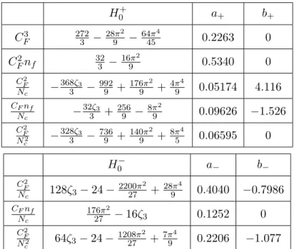
written in the following general form H ^(k) _inv f (z ₁ , z ₂ ) = Γ ^(k) _cusp

Z 1 0

dα α ¯ α

2f(z ₁ , z ₂ ) − f (z ^α ₁₂ , z ₂ ) − f (z ₁ , z ₂₁ ^α )

+ χ ^(k) ₀ f (z ₁ , z ₂ ) +

Z 1 0

dα Z α ¯

0

dβ

χ ^(k) _inv (τ ) + χ ^P _inv ^(k) (τ ) P 12

f(z ₁₂ ^α , z ^β ₂₁ ) . (3.13) Here z ₁₂ ^α is defined in eq. (2.10), τ = αβ/( ¯ α β ¯ ) and P 12 is the permutation operator, P 12 f (z 1 , z 2 ) = f (z 2 , z 1 ). Γ cusp is the cusp anomalous dimension which is known to the required accuracy [6]:

Γ ⁽¹⁾ _cusp = 4C F , Γ ⁽²⁾ _cusp = 16

C _A C _F

67 36 − π ²

12

− 5 18 n _f C _F

, Γ ⁽³⁾ _cusp = 64

C _A ² C _F

245

96 − 67π ²

216 + 11π ⁴ 720 + 11

24 ζ ₃

+ C _A C _F n _f 1 2

− 209 216 + 5π ²

54 − 7 6 ζ ₃

+ C _F ² n _f 1 2

ζ ₃ − 55 48

− 1 108 C _F n ² _f

. (3.14)

The LO expression (2.13) corresponds to

χ ⁽¹⁾ ₀ = 2C _F , χ ⁽¹⁾ _inv (τ ) = −4C _F , χ ^P(1) _inv (τ ) = 0 . (3.15) The two-loop constant term χ ⁽²⁾ ₀ and the functions χ ⁽²⁾ _inv (τ ), χ ^P _inv ⁽²⁾ (τ ) are given in appendix A.

The three-loop expressions will be derived below.

Note that the expression for the two-loop kernel in eq. (3.12) differs from the one derived in ref. [15] where the non-invariant part is written in form of a single expression.

The representation of the non-invariant part of the two- and three-loop kernel as a product of simpler operators suggested here seems to be sufficient and probably more convenient for most applications.

4 Reciprocity relation

The eigenvalues of H ^(k)

H ^(k) (z 1 − z 2 ) ^N = γ ^(k) (N ) (z 1 − z 2 ) ^N (4.1) correspond to the flavor-nonsinglet anomalous dimensions in the MS scheme that are known to three-loop accuracy [6]. Note that our definition of the anomalous dimension γ ^(k) (N ) differs from the one used in ref. [6] by an overall factor of two. In addition, in our work N refers to the number of derivatives whereas in [6] the anomalous dimensions are given as functions of Lorentz spin of the operator. Thus

γ ^(k) (N )

this work = 2 γ ^(k) (N + 1)

ref. [6] . (4.2)

JHEP06(2017)037

One can show that the eigenvalues of the invariant kernels H ⁽³⁾ _inv

H ^(k) _inv (z ₁ − z ₂ ) ^N = γ _inv ^(k) (N ) (z ₁ − z ₂ ) ^N (4.3) with a “natural” choice of T operators specified in appendix C satisfy the following sym- metry relation: let j _N = N + 2 (conformal spin); the asymptotic expansion of γ _inv ^(k) (N ) at large j → ∞ only contains terms symmetric under the replacement j N → 1 − j N . Note that this symmetry does not hold for the anomalous dimensions γ ^(k) (N ) themselves.

The argument goes as follows. As well known [28], conformal symmetry implies that the evolution kernels can be expressed in terms of the quadratic Casimir operator of the symmetry group. As a consequence it is natural to parameterize the anomalous dimensions in the form

γ(N ) = f

N + 2 + ¯ β(a) + 1 2 γ (N )

= f

j N + ¯ β(a) + 1 2 γ(N )

. (4.4)

It has been shown [18–20] that the asymptotic expansion of the function f(j) = af ⁽¹⁾ (j) + a ² f ⁽²⁾ (j) +. . . at large j only contains terms that are symmetric under reflection j → 1 − j.

In all known examples the f -function also proves to be simpler than the anomalous dimen- sion itself. Expanding both sides of eq. (4.4) in a power series in the coupling one obtains ²

f ⁽¹⁾ (j N ) = γ ⁽¹⁾ (N) , (4.5a)

f ⁽²⁾ (j N ) = γ ⁽²⁾ (N)− d dN

β 0 + 1

2 γ ⁽¹⁾ (N ) 2

= γ ⁽²⁾ (N )−

β 0 + 1

2 γ ⁽¹⁾ (N ) d

dN f ⁽¹⁾ (j N ) , (4.5b) f ⁽³⁾ (j _N ) = γ ⁽³⁾ (N)−

β ₁ + 1

2 γ ⁽²⁾ (N ) d

dN f ⁽¹⁾ (j _N )− 1 2

β ₀ + 1

2 γ ⁽¹⁾ (N ) 2

d ²

dN ² f ⁽¹⁾ (j _N )

−

β ₀ + 1

2 γ ⁽¹⁾ (N) d

dN f ⁽²⁾ (j _N ) , (4.5c)

so that the values of f ^(k) (j _N ) are related to the anomalous dimensions at the same order of perturbation theory up to subtractions of certain lower-order terms.

Let us compare this expansion with the relations between the eigenvalues of H ^(k) in eq. (4.1) and of the invariant kernel H ^(k) _inv in eq. (4.3). Using eq. (3.12) and explicit expressions for the eigenvalues of the T kernels in eq. (C.6) one obtains (note that the commutator terms do not contribute to the spectrum)

γ ⁽¹⁾ (N ) = γ _inv ⁽¹⁾ (N ) , γ ⁽²⁾ (N ) = γ _inv ⁽²⁾ (N ) +

β 0 + 1

2 γ ⁽¹⁾ (N ) d

dN γ _inv ⁽¹⁾ (N ) , γ ⁽³⁾ (N ) = γ _inv ⁽³⁾ (N ) +

β ₁ + 1

2 γ _inv ⁽²⁾ (N ) d

dN γ _inv ⁽¹⁾ (N ) + 1 2

β ₀ + 1

2 γ _inv ⁽¹⁾ (N ) 2

d ²

dN ² γ _inv ⁽¹⁾ (N ) +

β 0 + 1

2 γ _inv ⁽¹⁾ (N ) d

dN γ _inv ⁽²⁾ (N ) + 1 2

d

dN γ _inv ⁽¹⁾ (N) 2

. (4.6)

2

See also ref. [17] for a derivation in terms of the corresponding splitting functions in x-space.

JHEP06(2017)037

Comparing this expansion to the one in eq. (4.5) we see that

f ^(k) (j _N ) = γ _inv ^(k) (N ) . (4.7) In other words, the QCD anomalous dimension in the MS scheme can be written in terms of the eigenvalues of the invariant kernel as

γ(N ) = γ inv

N + 2 + ¯ β(a) + 1 2 γ (N )

, (4.8)

and the asymptotic expansion of γ _inv (N ) at large N only contains terms invariant under the reciprocity transformation j _N = N + 2 7→ 1 − j _N = −N − 1 [18–20].

This relation implies a certain condition for the choice of T kernels which appears to be natural in the first few orders of perturbation theory, see appendix C.

5 Three-loop invariant kernel H ⁽³⁾ _inv

The three-loop invariant kernel H ⁽³⁾ _inv takes the form H ⁽³⁾ _inv f (z 1 , z 2 ) = Γ ⁽³⁾ _cusp

Z 1 0

dα α ¯ α

2f (z 1 , z 2 ) − f (z ₁₂ ^α , z 2 ) − f(z 1 , z ₂₁ ^α )

+ χ ⁽³⁾ ₀ f (z 1 , z 2 ) +

Z 1 0

dα Z α ¯

0

dβ

χ ⁽³⁾ _inv (τ ) + χ ^P _inv ⁽³⁾ (τ )P 12

f (z ₁₂ ^α , z ₂₁ ^β ) . (5.1) The three-loop cusp anomalous dimension Γ ⁽³⁾ cusp is known (3.14) so that our task is to determine the constant χ ⁽³⁾ ₀ and two functions of one variable, χ ⁽³⁾ _inv (τ ) and χ ^P(3) _inv (τ ). This can be done by using the information on the spectrum of H ⁽³⁾ _inv

H ⁽³⁾ _inv (z 1 − z 2 ) ^N = γ _inv ⁽³⁾ (N ) (z 1 − z 2 ) ^N , (5.2) where

γ _inv ⁽³⁾ (N ) = γ ⁽³⁾ (N ) −

β 1 + 1

2 γ ⁽²⁾ (N ) d

dN γ ⁽¹⁾ (N ) −

β 0 + 1

2 γ ⁽¹⁾ (N ) d

dN γ ⁽²⁾ (N ) + 1

2

β 0 + 1

2 γ ⁽¹⁾ (N ) d

dN γ ⁽¹⁾ (N ) 2

(5.3) can easily be calculated from the known one-, two-, and three-loop flavor-nonsinglet anoma- lous dimensions [6].

The constant term χ ⁽³⁾ ₀ in the invariant kernel (5.1) corresponds to the constant term in the large-N asymptotic of the anomalous dimension

γ _inv ⁽³⁾ (N ) = 2 Γ ⁽³⁾ _cusp h

ψ(N + 2) − ψ(2) i

+ χ ⁽³⁾ ₀ + O(1/N ² ) (5.4)

JHEP06(2017)037

and is straightforward to obtain. Using the expressions from ref. [6] we find χ ⁽³⁾ ₀ = C _F ³

3176

9 ζ 3 − 320ζ 5 + 1672π ⁴

135 − 23954π ²

81 + 13454 9

+ C _F ² n _f

− 752

9 ζ 3 − 128π ⁴

135 + 3452π ²

81 − 6242 27

+ C _F n ² _f 32

9 ζ 3 − 80π ² 81 + 70

27

+ C _F ² N c

− 16

3 π ² ζ ₃ + 9464

9 ζ ₃ − 560ζ ₅ + 322π ⁴

27 − 27158π ²

81 + 28789 18

+ C _F n _f N c

− 1072

9 ζ 3 − 2π ⁴

45 + 1816π ²

81 − 2752 27

+ C F

N _c ² 3632

9 ζ 3 − 80ζ 5 + 31π ⁴

15 − 7712π ²

81 + 7537 18

. (5.5)

The calculation of the functions χ ⁽³⁾ _inv (τ ) and χ ^P _inv ⁽³⁾ (τ ) is much more involved. As usual one has to consider even and odd values of N separately. We write

γ _inv ⁽³⁾ (N ) = γ _inv ⁽³⁺⁾ (N ) + (−1) ^N γ _inv ⁽³⁻⁾ (N ) , (5.6) so that the combinations γ ⁽³⁺⁾ _inv (N )±γ _inv ⁽³⁻⁾ (N ) correspond to the eigenvalues of the invariant kernel for even (odd) N. Using the representation in (5.1) one obtains

γ _inv ⁽³⁺⁾ (N ) = 2Γ ⁽³⁾ _cusp

ψ(N +2)−ψ(2)

+χ ⁽³⁾ ₀ + Z 1

0

dα Z α ¯

0

dβ χ ⁽³⁾ _inv (τ ) (1−α−β) ^N , (5.7a) γ _inv ⁽³⁻⁾ (N ) =

Z 1 0

dα Z α ¯

0

dβ χ ^P(3) _inv (τ ) (1−α−β) ^N . (5.7b)

These relations can be inverted to express the kernels as functions of the anomalous di- mensions [15]

χ ⁽³⁾ _inv (τ ) = 1 2πi

Z c+i∞

c−i∞

dN (2N + 3) ∆γ _inv ⁽³⁺⁾ (N ) P _N+1

1 + τ 1 − τ

, χ ^P _inv ⁽³⁾ (τ ) = 1

2πi

Z c+i∞

c−i∞

dN (2N + 3) γ _inv ⁽³⁻⁾ (N ) P N +1

1 + τ 1 − τ

, (5.8)

where

∆γ _inv ⁽³⁺⁾ (N ) = γ _inv ⁽³⁺⁾ (N ) − 2Γ ⁽³⁾ _cusp

ψ(N + 2) − ψ(2)

− χ ⁽³⁾ ₀ , (5.9) and P N +1 is the Legendre function. All singularities of the anomalous dimensions have to lie to the left of the integration contour.

The algebraic structure of the three-loop anomalous dimension γ _inv ⁽³⁾ (N ) [6] is, unfortu- nately, too complicated to do the integrals in (5.8) analytically. We, therefore, adopted the following strategy: we will provide analytic expressions for the terms that correspond to

1. the leading contributions ∼ (ψ(j)−ψ(2))

j(j−1) , j = N + 2, to the large-N expansion of the anomalous dimensions,

2. the contribution of the leading singularity (pole at N = −1) in the complex plane.

The remainder will be parameterized by a sufficiently simple function with a few fit

parameters.

JHEP06(2017)037

5.1 Splitting functions

It turns out to be advantageous to use the representation for the anomalous dimensions in terms of the splitting functions. The three-loop splitting functions are available from ref. [6] and involve harmonic polylogarithms (HPL) up to weight five, see ref. [29]. Using this result and eq. (5.3) it is straightforward to calculate the splitting functions for the invariant kernels such that

γ _inv ^(3±) (N ) = − Z 1

0

dx x ^N H _inv ^(3±) (x) . (5.10) The “plus” function can be written as

H _inv ⁽³⁺⁾ (x) = 2Γ ⁽³⁾ _cusp x

(1 − x) ₊ − χ ⁽³⁾ ₀ − 2Γ ⁽³⁾ _cusp

δ(1 − x) + ∆H _inv ⁽³⁺⁾ (x) , (5.11) where the first two terms are related to the logarithmic and the constant contributions in the large-N expansion of the anomalous dimension, cf. (5.7a) and for H _inv ⁽³⁻⁾ (x) there are no such terms, cf. (5.7b). The symmetry property under j _N 7→ 1 − j _N for the eigenvalues of the invariant kernel is equivalent to the Gribov-Lipatov reciprocity relation for the corresponding splitting functions

∆H _inv ^(3±) (x) = −x∆H _inv ^(3±) (1/x) . (5.12) We want to find a parametrization for the splitting functions consistent with the reciprocity relations (5.12) and separating the leading contributions at x → 0 and x → 1.

To this end, let us define the set of functions φ _k (x) such that Z 1

0

dx x ^j−2 φ k (x) = 1

j(j − 1) k+1

. (5.13)

They can be constructed recursively,

φ 0 (x) = 1 − x , φ _k (x) = Z 1

x

dξ

ξ φ k−1 (ξ)φ 0 (x/ξ) , (5.14) so that

φ 1 (x) = −2¯ x − (1 + x) ln x ,

φ 2 (x) = 2¯ x ² + ¯ x(3 + x) ln x + (1 + x) ln ² x , (5.15) where here and below

¯

x = 1 − x . (5.16)

We write the splitting functions as

∆H _inv ⁽³⁺⁾ (x) =

4

X

k=1

B _k ⁽³⁺⁾ φ _k (x) + ¯ x C ₀ ⁽³⁺⁾ + ¯ x C ₁ ⁽³⁺⁾ ln x

¯ x ²

+ δH _inv ⁽³⁺⁾ (x) ,

H _inv ⁽³⁻⁾ (x) =

4

X

k=1

B _k ⁽³⁻⁾ φ k (x) + ¯ x C ₀ ⁽³⁻⁾ + δH _inv ⁽³⁻⁾ (x) , (5.17)

JHEP06(2017)037

Figure 1. Left panel shows the ratio δH _inv ⁽³⁺⁾ (x)/H _inv ⁽³⁺⁾ (x) (dashed curve) for exact splitting func- tions and the error in using the approximation (5.22) , (δH _inv ⁽³⁺⁾ | fit − δH _inv ⁽³⁺⁾ | exact )/H _inv ⁽³⁺⁾ (solid curve) for n f = 4. The shaded area indicates an error band of 0.5%. The similarly defined approx- imation error for the combinations H ⁽⁺⁾ + H ⁽⁻⁾ (dashes) and H ⁽⁺⁾ − H ⁽⁻⁾ (solid) which give rise to moments with odd and even N , respectively, is shown on the right panel.

where the addenda, δH _inv ⁽³⁺⁾ (x) and δH _inv ⁽³⁻⁾ (x), do not include, by construction, terms ln ^k x, k ≥ 1 (for x → 0) and ¯ x ln ^k x, ¯ k ≥ 0 (for x → 1). The maximum powers of the logarithms are found by inspection of the known analytic expression. Thus, with normalization constants H ₀ ^±

δH _inv ^(3±) (x) =

x→1 O(¯ x ³ ) , δH _inv ^(3±) (x) =

x→0 H ₀ ^± + O(x) , (5.18) or, equivalently, in moment space,

δγ _inv ^(3±) (N ) = − Z 1

0

dx x ^N δH _inv ^(3±) (x) , (5.19) vanishes as 1/N ⁴ at large N and its only possible singularity at N = −1 is a simple pole.

The constants B ^(3±) _k , C _k ^(3±) are collected in table 1 where, for completeness, we also repeat the expressions for χ ⁽³⁾ ₀ (5.5) and Γ ⁽³⁾ cusp (3.14). In all cases we show the coefficients for the following color decomposition:

F = C _F ³ F h1i + C _F ² n f F h2i + C F n ² _f F h3i + C _F ² N c

F h4i + C _F n _f N c

F h5i + C _F

N _c ² F h6i , (5.20) where F = A ^(3±) _k , B _k ^(3±) , χ ⁽³⁾ ₀ , Γ ⁽³⁾ cusp .

The remaining terms δH _inv ^(3±) (x) contain the whole algebraic complexity of the full result but numerically they are rather small. For illustration we show the ratio δH _inv ⁽³⁺⁾ (x)/H _inv ⁽³⁺⁾ (x) for N c = 3 and n f = 4 in figure 1 (dashed blue curve on the left panel). One sees that δH _inv ⁽³⁺⁾ (x) contributes at most 6% to the full splitting function in the whole range 0 < x < 1 so that for all practical purposes it can be approximated by a simple expression with a few parameters.

Due to the reciprocity property (5.12) the functions δH _inv ^(3±) (x) can be parameterized in the form

δH _inv ^(3±) (x) = ¯ x h ± (x/¯ x ² ) . (5.21)

JHEP06(2017)037

χ ⁽³⁾ ₀ Γ ⁽³⁾ cusp

C _F ^{3 3176} ₉ ζ 3 − 320ζ 5 + ^1672π ₁₃₅

− ^23954π ₈₁

+ ¹³⁴⁵⁴ ₉ ³⁵² ₃ ζ 3 + ¹⁹⁶⁰ ₃ − ^2144π ₂₇

+ ^176π ₄₅

C _F ² n f − ⁷⁵² ₉ ζ 3 − ^128π ₁₃₅

+ ^3452π ₈₁

− ⁶²⁴² ₂₇ − ¹²⁸ ₃ ζ 3 − ²⁶⁶² ₂₇ + ^160π ₂₇

C _F n ² _f ³² ₉ ζ ₃ − ^80π ₈₁

+ ⁷⁰ ₂₇ − ¹⁶ ₂₇

C

N

− ^16π ₃

ζ ₃ + ⁹⁴⁶⁴ ₉ ζ ₃ − 560ζ ₅ + ^322π ₂₇

− ^27158π ₈₁

+ ²⁸⁷⁸⁹ ₁₈ ³⁵² ₃ ζ ₃ + ¹⁹⁶⁰ ₃ − ^2144π ₂₇

+ ^176π ₄₅

C

n

N

− ¹⁰⁷² ₉ ζ ₃ − ^2π ₄₅

+ ^1816π ₈₁

− ²⁷⁵² ₂₇ − ¹¹² ₃ ζ ₃ − ⁸³⁶ ₂₇ + ^80π ₂₇

C

N

3632

9 ζ ₃ − 80ζ ₅ + ^31π ₁₅

− ^7712π ₈₁

+ ⁷⁵³⁷ ₁₈ ⁸⁸ ₃ ζ ₃ + ⁴⁹⁰ ₃ − ^536π ₂₇

+ ^44π ₄₅

B ₁ ⁽³⁺⁾ B ₂ ⁽³⁺⁾ B ₃ ⁽³⁺⁾ B ₄ ⁽³⁺⁾ C ₀ ⁽³⁺⁾ C ₁ ⁽³⁺⁾ C _F ³ − ⁷⁴⁶ ₉ − ^40π ₉

20 − ^16π ₃

0 0 ³⁵² ₃ ζ ₃ + ⁷⁰⁷⁶⁸ ₂₇ − ^3488π ₂₇

+ ^176π ₄₅

− ¹⁸⁴ ₃ C _F ² n _f ²⁸ ₉ − ^16π ₉

0 0 0 − ¹²⁸ ₃ ζ ₃ − ¹¹⁹⁶⁶ ₂₇ + ^256π ₂₇

− ¹⁶ ₃

C _F n ² _f 0 0 0 0 ⁶⁴ ₉ 0

C

N

−176ζ ₃ + ¹⁸⁸⁶ ₃ − ^52π ₉

³⁶³² ₉ − ^16π ₃

− ⁵²⁰ ₃ −64 ³⁵² ₃ ζ ₃ + ⁷⁴⁴²⁸ ₂₇ − ^3488π ₂₇

+ ^176π ₄₅

^16π ₃

− ³⁷⁶ ₃

C

n

N

− ⁵¹² ₉ − ^8π ₉

− ⁴⁰⁰ ₉ − ¹⁶ ₃ 0 − ¹¹² ₃ ζ ₃ − ⁵⁹³² ₂₇ + ^128π ₂₇

− ⁸ ₃

C

N

−112ζ ₃ + ³²⁷² ₉ − ^76π ₉

¹⁸¹⁶ ₉ − ^16π ₃

− ¹⁷⁶ ₃ −24 ⁸⁸ ₃ ζ ₃ + ¹⁷⁹⁰² ₂₇ − ^836π ₂₇

+ ^44π ₄₅

^8π ₃

− ¹⁹⁶ ₃ B ₁ ⁽³⁻⁾ B ₂ ⁽³⁻⁾ B ₃ ⁽³⁻⁾ B ₄ ⁽³⁻⁾ C ₀ ⁽³⁻⁾

C

N

−128ζ ₃ + ⁷²⁸⁸ ₉ + ^52π ₉

³⁶³² ₉ + ^32π ₃

− ⁵²⁰ ₃ −64 ⁸⁸ ₃

C

n

N

16π

9 − ⁴⁸⁸ ₉ − ⁴⁰⁰ ₉ − ¹⁶ ₃ 0 − ⁸ ₃

C

N

−112ζ ₃ + ³⁸⁶⁰ ₉ + ^164π ₉

¹⁸¹⁶ ₉ + ^44π ₃

− ¹⁷⁶ ₃ −24 ⁴⁴ ₃

Table 1. Cusp anomalous dimension Γ ⁽³⁾ cusp (3.14) , constant term χ ⁽³⁾ ₀ (5.5) and the coefficients B _k ^(3±) , C _k ^(3±) (5.17) in the splitting function representation of the invariant kernel.

We choose the following ansatz

h ± (t) = H ₀ ^± a ±

t + a ±

1 + b ± t t + a ±

, (5.22)

where a ± and b ± are fit parameters and the normalization constants H ₀ ^± are determined analytically from the condition δH _inv ^(3±) (x) =

x→0 H ₀ ^± + O(x) (5.18). The fitted values of the parameters a ± and b ± for the different color structures can be found in table 2. With this simple parametrization we reduce the deviation from the exact splitting functions to less than 0.5%, see figure 1.

5.2 Mellin transformation

The following Mellin representation of the kernels χ inv (τ ) and χ ^P _inv (τ ) proves to be useful

in order to restore them from the splitting functions and allows one to write all terms in

JHEP06(2017)037

H ₀ ⁺ a + b +

C _F ^{3 272} ₃ − ^28π ₉

− ^64π ₄₅

0.2263 0 C _F ² n _f ³² ₃ − ^16π ₉

0.5340 0

C

N

− ^368ζ ₃

− ⁹⁹² ₉ + ^176π ₉

+ ^4π ₉

0.05174 4.116

C

n

N

− ^32ζ ₃

+ ²⁵⁶ ₉ − ^8π ₉

0.09626 −1.526

C

N

− ^328ζ ₃

− ⁷³⁶ ₉ + ^140π ₉

+ ^8π ₅

0.06595 0

H ₀ ⁻ a − b −

C

N

128ζ ₃ − 24 − ^2200π ₂₇

+ ^28π ₉

0.4040 −0.7986

C

n

N

176π

27 − 16ζ ₃ 0.1252 0

C

N

64ζ ₃ − 24 − ^1208π ₂₇

+ ^7π ₉

0.2206 −1.077

Table 2. Values of the parameters in the ansatz for δH _inv ^(3±) (x) (5.21) , (5.22) . the form that automatically respects the reciprocity relation:

χ(τ ) = 1 2πi

Z c+i∞

c−i∞

dρ χ(ρ) (¯ e τ /τ ) ^−ρ , (5.23a)

χ(ρ) = e Z 1

0

dτ

τ τ ¯ (¯ τ /τ ) ^ρ χ(τ ) . (5.23b) The integration contour in the first integral, (5.23a), must be chosen in the analyticity strip of the second integral, (5.23b), (the strip where integral converges). Making use of this representation one obtains

∆γ _inv ⁽³⁺⁾ (N ) = 1 2πi

Z c+i∞

c−i∞

dρ χ e ⁽³⁾ _inv (ρ)Γ ² (1 + ρ) Γ(j _N − 1 − ρ)

Γ(j N + 1 + ρ) , (5.24a) γ _inv ⁽³⁻⁾ (N ) = 1

2πi

Z c+i∞

c−i∞

dρ χ e ^P _inv ⁽³⁾ (ρ)Γ ² (1 + ρ) Γ(j _N − 1 − ρ)

Γ(j _N + 1 + ρ) . (5.24b) Since for large j _N the ratio Γ(j _N − 1 − ρ)/Γ(j _N + 1 + ρ) ∼ j _N ^−2(1+ρ) , the asymptotic expan- sion of the integrals in eqs. (5.24) at j N → ∞ can be obtained by moving the integration contour to the right and picking up the corresponding residues. It is easy to check that if the only singularities of the Mellin-transformed kernels χ(ρ) in the right half-plane are e poles (of arbitrary order) at real integer values of ρ, then a generic term of the asymptotic expansion of the anomalous dimensions has the form

(ψ(j N ) − ψ(1)) ^m

(j N (j N − 1)) ^k , k > 0, m ≥ 0 ,

which is required by the reciprocity symmetry under the j _N 7→ 1−j _N transformation [18–20].

Under the same condition ( χ(ρ) only has poles at integer e ρ values in the right half-plane),

JHEP06(2017)037

the kernels χ(τ ) at small values of the conformal ratio have the expansion χ(τ ) = X

km

c _km τ ^k ln ^m τ . The Mellin transform of the one-loop kernel is very simple:

χ ⁽¹⁾ _inv = −4C _F ↔ χ e ⁽¹⁾ _inv = −4C _F h

2πiδ(ρ) i

. (5.25)

More examples are collected in table 3, see appendix A. One finds that the Mellin space kernels have a rather simple form, while the corresponding anomalous dimensions can be quite involved. Also the two-loop evolution kernels in Mellin space are given by rather compact expressions, see eq. (A.3).

If the anomalous dimensions are written in terms of the splitting functions, eq. (5.10), γ _inv ^(k±) (N ) = −

Z 1 0

dx x ^N H _inv ^(k±) (x) , (5.26) the corresponding Mellin-transformed invariant kernels can be calculated as

χ e ^(k) _inv (ρ) = − Γ(2ρ + 2) Γ ² (1 + ρ)

Z 1 0

dx H _inv ^(k+) (x) 1 x¯ x

1 + x 1 − x

x

¯ x ²

ρ

(5.27) and similar for χ e ^P _inv ^(k) (ρ), with the replacement H _inv ^(k+) (x) → H _inv ^(k−) (x). The kernels in τ space can finally be obtained by the inverse Mellin transformation (5.23a). We found this two-step approach to be the most effective for the three-loop case.

For the remainder function δH _inv ^(3±) (x) written in the form (5.21) one obtains in Mellin space

δ χ e ^(3±) _inv (ρ) = − Γ(2ρ + 2) Γ ² (1 + ρ)

Z ∞ 0

dt h ± (t) t ^ρ−1 , (5.28) and for the simple ansatz in eq. (5.22)

δ χ e ^(3±) _inv (ρ) = − Γ(2ρ + 2) Γ ² (1 + ρ)

π

sin(πρ) H ₀ ^± (1 + b ± ρ)a ^ρ _± . (5.29) Using eq. (5.23a) we finally obtain the following expression for the corresponding contri- bution to the invariant kernel

δχ ^(3±) _inv (τ ) = H ₀ ^± (1 + 4a ± τ /¯ τ ) ^5/2

h 1 + a ±

τ

¯

τ (4 − 6 b ± ) i

− H ₀ ^± . (5.30) We also need the expressions for the functions φ k (5.14) in ρ- and τ -space defined as

φ e _k (ρ) ≡ − Γ(2ρ + 2) Γ ² (1 + ρ)

Z 1 0

dx φ _k (x) 1 x¯ x

1 + x 1 − x

x

¯ x ²

ρ

≡ Z 1

0

dτ

τ τ ¯ (¯ τ /τ ) ^ρ ϕ _k (τ ) . (5.31)

JHEP06(2017)037

One obtains

φ e 1 (ρ) = −π/(ρ sin πρ), φ e 2 (ρ) = φ e 1 (ρ) ρ ¯

ρ , φ e 3 (ρ) = φ e 1 (ρ)

− 2 ρ ¯

ρ + ψ ⁰ (ρ) − π ² 6

, φ e ₄ (ρ) = φ e ₁ (ρ)

5 ρ ¯

ρ + (1 − 3ρ) ρ

ψ ⁰ (ρ) − π ² 6

, (5.32)

and

ϕ 1 (τ ) = ln ¯ τ = H 1

− τ

¯ τ

, ϕ 2 (τ ) = −ϕ ₁ (τ ) + H 01

− τ

¯ τ

= − ln ¯ τ + Li 2 (−τ /¯ τ ) , ϕ 3 (τ ) = −2ϕ ₂ (x) − H 101

− τ

¯ τ

= 2H 1

− τ

¯ τ

− 2H 01

− τ

¯ τ

− H 101

− τ

¯ τ

,

= 2 ln ¯ τ − 2 Li 2 (−τ /¯ τ ) − 2

Li 3 (¯ τ ) − Li 3 (1)

+ ln ¯ τ

Li 2 (¯ τ ) + π ² 6

+ 1

6 ln ³ τ ¯ ϕ ₄ (τ ) = −3ϕ ₃ (τ ) − ϕ ₂ (τ ) − H ₀₁₀₁

− τ

¯ τ

= −5H ₁

− τ

¯ τ

+ 5H ₀₁

− τ

¯ τ

+ 3H ₁₀₁

− τ

¯ τ

− H ₀₁₀₁

− τ

¯ τ

, (5.33)

where H _p...q (z) are harmonic polylogarithms, see ref. [29].

With these expressions at hand, our result for the invariant kernel (5.1) is complete.

We obtain

χ ⁽³⁾ _inv (τ ) =

4

X

k=1

B _k ⁽³⁺⁾ ϕ _k (τ ) − C ₀ ⁽³⁺⁾ + C ₁ ⁽³⁺⁾

ln (τ /¯ τ ) + 2

+ δχ ⁽³⁺⁾ _inv (τ ) ,

χ ^P _inv ⁽³⁾ (τ ) =

4

X

k=1

B _k ⁽³⁻⁾ ϕ _k (τ ) − C ₀ ⁽³⁻⁾ + δχ ⁽³⁻⁾ _inv (τ ) , (5.34) where the functions ϕ _k (τ ) are defined in eq. (5.33), the coefficients B _k ^(3±) , C _k ^(3±) can be found in table 1 and the parameters for δχ ^(3±) _inv (τ ) (5.30) are collected in table 2.

For illustration, in figure 2 we compare the full NNLO invariant functions χ(a) = aχ ⁽¹⁾ + a ² χ ⁽²⁾ + a ³ χ ⁽³⁾ with the NLO, O(a ² ), and the LO, O(a), results for a typ- ical value of the coupling α s /π = 0.1 and, for definiteness, n f = 4. In the same plot the NNLO results using the exact three-loop functions obtained by the numerical integration of eq. (5.8) are shown by dots. One sees that the accuracy of our parametrization is rather good. The remaining entries in the invariant kernel are, for the same values n f = 4 and α _s /π = 0.1,

Γ _cusp = aΓ ⁽¹⁾ (1 + 8.019a + 80.53a ² + . . .) = aΓ ⁽¹⁾ (1 + 0.2005 + 0.0503 + . . .) ,

χ 0 = aχ ⁽¹⁾ ₀ (1 − 0.7935a − 141.3a ² + . . .) = aχ ⁽¹⁾ ₀ (1 − 0.0198 − 0.0883 + . . .) . (5.35)