Development of an Energy dependent Final State Distribution for T2

(1)

Development of an Energy dependent Final State Distribution for T

₂

Master Thesis

Technische Universit¨ at M¨ unchen

Cornelius Sch¨ atz

supervised by

Prof. Dr. Susanne Mertens

January 18, 2019

(2)

Abstract

In the search for dark matter, there arose many theoretical models over the course of the past centuries. One of those models includes the existence of a right-handed partner to the neutrino, the so called sterile neutrino. Its main property is, that it nearly doesn’t interact with the active neutrino flavours or other Standard Model particles. There are many hypothesises, in which range the mass of such a sterile neutrino could be. With beta decay experiments like the KATRIN experiment, it could be possible, to detect the signature of a sterile neutrino in the energy spectrum of the electron. Since the KATRIN experiment is using molecular tritium, one tritium atom decays into a³He atom, whereas the other one remains. The new molecule, that arises, contains an orbital electron, whose eigenstates and eigenvalues change due to the decay. The energy of the orbital electron has a slight impact on the energy of the escaping beta electron and thus has to be respected. After the decay, the orbital electron can be in many excited states, each with a certain probability.

The probability distribution of an orbital electron to end up in a certain excited state after the decay is called the Final States Distribution (FSD). The FSD has so far been calculated corresponding to beta electrons with an energy of 18.6 keV, allowing a more detailled analysis of the decay spectrum in the measurement of the neutrino mass. In order to look for a sterile neutrino with a keV mass, whose impact on the spectrum is far below the endpoint energy, the FSD needs to be known for different energies of the beta electron. The aim of this work is to develop a simplified model for this so called energy-dependent Final State Distribution. In the first chapter a short introduction to the physics of neutrinos and sterile neutrinos is given. In the second chapter, the experimental setup of the KATRIN experiment is described as well as the TRISTAN project, whose goal it is to redesign KATRIN in way, that it will be able to detect sterile neutrinos. In the third chapter, an introduction calculation of the FSD is given, followed by the development of a simplified model for the energy dependence of the groundstate FSD and of the first five excited states.

(5)

Chapter 1 Theory of Neutrinos and sterile neutrinos

Our understanding of neutrinos and the underlying physics has changed over the past few decades, still some of its most fundamental properties like the mass re- main unknown. Another question that pops up when working on neutrinos is the existence of a right-handed partner. Understanding those properties is essential on the way to get a feeling for the origin of particle masses as well as for the role of primordial neutrinos and there influence on the evolution of large scale structures in the universe. A discovery of the right-handed partner of the neutrino with a mass in an keV range could unlock the secret nature of dark matter. This chapter shall give a short introduction to the theory of neutrinos and sterile neutrinos which will be a motivation for the following work. First, the history of the neutrino will be explained, going on to the theory of neutrino oscillations and their relation to a non-zero neutrino mass. The correlation between determining the mass of the neutrino and β decay experiments will be explained. After that, the concept of sterile neutrinos, which are the right-handed partners of the neutrinos, will be described.

Their role as a possible dark matter candidate and their correlation to the β decay energy spectrum will be explained.

(6)

1.1 History of neutrino physics

The first time, the idea of the neutrino was postulated was in the year 1930 by Wolfgang Pauli [13]. Trying to describe the continous energy spectrum of the electron in aβ decay process, he assumed the existence of a new particle, which he then called a neutron. In his hypothesis, this particle was staying in the nucles, having no electrical charge and a spin ¹₂. As two years later the ”real” neutron was discoverd by Chadwick, being a neutral particle with a mass just slightly higher than the proton’s mass, Pauli changed the name of his particle to neutrino. Shortly after the discovery of the neutron, Fermi formulated the first quantum theoretical theory of β decays [14]. In this model, a massive neutral particle, being the neutron, decays into a proton, an electron and into a neutral, massless particle, called the neutrino ν, or to be more precise, into an anti-electron neutrino ¯νe.

n →p+e+ ¯νe (1.1)

In 1956, Cowan [15] discovered the existence of the inverse β decay.

p+ ¯νe →n+e⁺ (1.2)

In this process a proton and an anti-electron neutrino decay into a positron and a neutron. After the detection of a muon flavoured neutrino in 1962, the idea came up, that neutrinos, similarly to the leptons, occur in different flavours. The last neutrino flavour, called a tauon neutrino, was only discovered 20 years later, after remaining theoretical for a long time.

1.2 Neutrino oscillations

Neutrino oscillations were first predicted bei B. Pontecorvo [16]. The first experimental evidence was given about ten years later by experiments such as Homestake, SNO and Kamiokande. In the Homestake experiment the flux of solar electron neutrinos was measured. A high deficit of high energy neutrinos compared to the solar neutrino model was detected, often recalled as the solar neutrino problem.

The solution to that are the socalled neutrino oscillations. In this model, a neutrino of flavour x can turn with a certain probability into a neutrino with flavour y.

(7)

Mathematically, neutrino oscillations are explained using the PNMS (Pontecorvo- Magi-Nakagawa-Sakata) matrix Uli:

νl =

3

X

i=1

Uliνi (1.3)

with the index l indicating the flavour eigenstates of the neutrino (e,µ, τ) and i indicating the mass eigenstates. The equation in a written out form looks like:



 νe

νµ

ντ



=





Ue1 Ue2 Ue3

Uµ1 Uµ2 Uµ3

Uτ1 Uτ2 Uτ3







 ν1

ν2

ν3





In a simplified model of neutrino oscillations with only two flavour and mass eigenstates, the probability of a x flavoured neutrino oscillating into a y flavoured one would be:

P(νx →νy) =sin²(2θ)·sin²

1.27·∆m²_xy/eV² L/km Eν/GeV

(1.4) Eν denotes the energy of the neutrino, ∆m²_xy = m²_x −m²_y is the difference of the squared mass corresponding to the mass eigenstates and L is the distance the neutrino traveled. The variable θ stands for the mixing angle between the flavour eigenstates. Since the oscillation probability is dependent on the squared mass difference, one can deduce, that neutrino oscillations imply a non-zero mass of this particle.

Determining the neutrino mass is an aim of many experiments in the area of experimental neutrino research. Such experiments are divided into the kinematics of the escaping electron in β decay, half-life measurements in the neutrinoless double β decay (0νββ) and cosmological observations. Analyzing the energy spectrum of the electron in an nuclear β decay would directly yield the neutrino mass as an observable whereas other approaches like the cosmological observations indirectly measure the sum of all neutrino mass eigenstates and depend strongly on the used cosmological model.

In β decay, a neutron decays into a proton, emitting a W⁻ boson, which then decays into an electron and an anti-electron neutrino. The derivation of the differential spectrum of the tritium beta decay will be now explained shortly following [17]. Using Fermis Golden Rule, the decay rate is given by

Γ = 2πXZ

|M |² df (1.5)

(8)

with M being the transition matrix element andP R

df representing the sum (integral) over all possible discrete (continous) final states f. First focus on the termdf. Letdn be the number of different final states of outgoing particles inside a volume V into the solid angledΩ with momentum [p, p+dp]. One then can write

dn= V d³~p

h³ = V p²dpdΩ

h3 (1.6)

Using the relationE_tot² =m²+p² which impliespdp=EtotdEtot, this expression can be written as:

dn= V pEtotdEtotdΩ

(2π)³ (1.7)

The density of states in a certain energy interval and solid angle becomes:

dn

dEtotdΩ = V pEtot

(2π)³ (1.8)

Since the mass of the daughter nucleus is much higher than the energies of the two emitted leptons, it is a valid assumption to say that the nucles does not have any kinetic energy at all. The density of states for the electron and the neutrino becomes

ρ(Ee, EνdΩe, dΩν) = V²p

E_e²−m²_eEe

pE_ν²−m²_νEν

(2π)⁶ (1.9)

Let’s now focus on the matrix element M. This can be divided into a leptonic and a nuclear part:

M =GFcosθCMlepMnuc (1.10)

withθC denoting the Cabibbo angle. Since the decay of tritium is either a allowed or superallowed transition, means a decay in which none of the leptons has any angular momentum and both are treated as plane waves, the leptonic matrix elemenent becomes:

|Mlep |²= 1

V²F(E, Z⁰) (1.11)

F(E, Z⁰) is denoting the Fermi function, which describes the Coulomb interaction of the beta electron and the daughter nucleus having an atomic number Z’. In an allowed or superallowed transition the nuclear matrix element is not dependent on the energy of the escaping electron. It can thus be divided into a Fermi part (with the nuclear spin difference being zero) and a Gamov-Teller part (with a nuclear spin

(9)

difference being either zero or ±1). What remains, is an angular correlation of the two outgoing leptons. The directions of the leptons are connected to each other via the factor:

1 +a(β~e·β~ν) (1.12)

with βi =vi/c and a being 1 for pure Fermi transitions and -1/3 for pure Gamov- Teller transitions according to [18]. With this knowledge it is possible to compute the partial decay rate Γ0 with P0 being the probability of this very decay channel:

Γ0 = 2πP0

Z

Ee,Eν,Ωe,Ων

|GFcosθCMlepMnuc |² dnednν = (1.13) P0

(2π)⁵ Z

Ee,Eν,Ωe,Ων

G²_Fcos²θCF(E, Z⁰)|Mnuc|² · (1.14) pE_e²−m²_eEe

pE_ν² −m²_νEν(1 +a~βeβ~ν)· (1.15) δ(Q−(Ee−me)−Eν −Erec)dEedΩedEνdΩν (1.16) Q stands for the energy released in the decay process. This energy is, according to the δ function, distributed into the kinetic energy of the electron, the total energy of the neutrino and the recoil energy of the daughter nucleus. What we are now actually interested in, is a formula for the differential energy spectrum of the escaping electron

dN

dtdE = dΓ

dE (1.17)

which gives the number of counts per time and energy unit. The differential decay spectrum takes the following form:

dΓ

dE =C·F(E, Z⁰)·pe·(E+me)·p

(E+me)²−m²_e· (1.18) (E0−E)·q

(E0−E²)²−m²_β (1.19) The constant C stands for the fraction ^G²^F^cos²_2π^θ^C3^|M^nuc^|². mβ is the effective neutrino mass, respectively

m²_β =X

i

|Uei |² m²_i (1.20)

summing over all flavours. Noting that in the decay process of a tritium atom bound in a T₂ molecule there is a orbital electron, which can be in several excited states

(10)

with energy Ef and probability Pf, the differential decay rate changes to:

dΓ

dE =X

f

Pf·C·F(Z, E)·p·Etot·(E0−E−Ef)·q

Θ(E0−E−Ef −mν)·((E0−E−Ef)²−m²_ν)) (1.21)

Measuring the electron energy spectrum will yield the total decay energy minus the energy of the anti-electron neutrino. Thus, the spectrum of the electron is shifted by the effective mass of the neutrino

mν¯e = v u u t

3

X

i=1

|Uei |M_νi² (1.22)

In the approach of measuring the neutrino mass using the neutrinoless double beta decay, one takes a look at the process of two neutrons decaying into two protons, two electrons anf two anti-electron neutrinos. The continous energy spectrum of the electron is shifted by two times the neutrino mass. If the neutrino is a Majorana fermion, meaning it is its own anti-particle, then the anti-electron neutrino might be directly absorbed in the second beta decay inside the nucleus. The emitted electrons would result in a mono-energetic line at the endpoint of the spectrum, with dacay rate of the neutrinoless double beta decay being proportional to the effective Majorana mass mββ.

In cosmological observations, like done by WMAP and the Planck Satellite. data from cosmic microwave background and baryonic acoustic oscillations were combined based on the ΛCDM model.

1.3 Sterile neutrinos

A natural extenstion of the Standard Model of particle physics (SM) would be the introduction of a right-handed neutrino, which from now on will be called sterile neutrinos. Those neutrinos are only sensitive to gravitational interaction. Sterile neutrinos make up a fourth mass eigenstateν4 with eigenvaluem4 and mix up with the other neutrino flavours. There are three possible models, which mass the sterile neutrino could have. Those are considering sterile neutrinos in the mass range of eV, keV and GeV. Sterile neutrinos with an electron-Volt mass could explain certain anomalies occuring in reactor experiments for example. If the sterile neutrino has

(11)

a mass in the range of kilo electron volts, they could be a viable candidate for dark matter. Giga electron volt sterile neutrinos could explain the small masses of the interacting neutrinos via the see-saw mechanism as well as being a solution for baryogenesis (the asymmetry between matter and anti-matter in our universe).

Since the aim of this work is to develop a model to possibly find keV sterile neutrinos, only these will be explained in some detail. Sterile neutrinos with a mass in the keV range would serve as warm dark matter, a scenario between cold and hot dark matter. The parameters of interest are its mass eigenvaluem4 as well as the active- sterile mixing amplitude sin²θs. The main effort of cosmological observations is to constrain the allowed region of these two free parameters. One can already guess, that the mixing amplitude is very small, since sterile neutrinos are not supposed to interact a lot with the other neutrino flavours. In the search for the mass of sterile neutrinos, the beta decay of tritium is with its endpoint energy of E0 = 18.6keV a perfect tool to probe the impact of an (still hypothetical) sterile neutrino. The mixing of the four neutrino flavours is described with an extended PMNS matrix:





 νe

νµ

ντ

νs







=







U_e1^∗ U_e2^∗ U_e3^∗ U_e4^∗ U_µ1^∗ U_µ2^∗ U_µ3^∗ U_µ4^∗ U_τ1^∗ U_τ2^∗ U_τ3^∗ U_τ4^∗ U_s1^∗ U_s2^∗ U_s3^∗ U_s4^∗











 ν1

ν₂ ν3

ν4





 One can then write

1 =

3

X

i=1

|U_ei² |+|Ue4 |:=cos²θs+sin²θs (1.23) withθs denoting the active-sterile mixing angle. It can be considered as an effective mixing of an active neutrino with mass mlight and sterile neutrino with mass m4, since it is not possible yet to resolve the light mass states. Having a look at the differential decay rate corresponding to the beta decay of tritium together with an influence of a sterile neutrino, it looks like:

dΓ

dE =cos²θs

dΓ

dE(m²_light) +sin²θs

dΓ

dE(m²₄) (1.24)

with dΓ

dE(m²₄) = C·F(E, Z⁰)·pe(E+me)p

(E+me)²−m²_e(E0−E) q

(E0 −E)²−m²₄ (1.25) The spectrum of a decay into a sterile neutrino (equation above) would have a lower endpoint, to be precise E0 −m4 and a really small amplitude sin²θs. Thus,

(12)

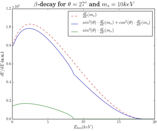
the impact of a sterile neutrino on the whole beta spectrum results in a kink-like signature at E0−m4 and a tiny distortion of the amplitude in the region between zero energy andE₀−m₄. This kink-like signature can be seen in Figure 1.1. A mass of 10 keV and a mixing angle of 27 degrees has been used. Although the mixing angle is extremely unrealistic, this example shows quite well the imprint of a sterile neutrino on the spectrum of the beta electron.

Figure 1.1: Differential decay rate for the beta decay of tritium without sterile neutrinos (red dashed) and with an sterile neutrino having a mass of 10 keV and a mixing angle of 27 degrees (which is unrealistic, but shows quite well the imprint of an sterile neutrino on the energy spectrum of the escaping electron)

Since tritium in reality occurs in molecular form, for example as aT2 molecule, the energy of the remaining orbital electron needs to substracted from the energy of the escaping electron, when having a look at the differential decay rate. This has a slight impact on the spectrum. The aim of this work will be to develop a simplified

(13)

model for the behaviour of the orbital electron after the decay in order to analyze the spectrum more detailled.

(14)

Chapter 2 The KATRIN experiment

The KArlsruhe TRItium Neutrino experiment (KATRIN) is a beta decay experiment with the goal to measure the effective mass of the anti-electron neutrino.This happens with the use of high precision spectroscopy of the beta electrons produced in the decay with an energy close to the endpoint E0. This chapter shall give a short introduction to the measurement principle of KATRIN and to the experimental setup.

2.1 Experimental setup

With the aim to detect tiny distortions of the tritium spectrum near the endpoint due to a non-zero effective neutrino mass, the KATRIN experiment implements a high countrate of a stable molecular trititum source combined with a changeable retarding potential acting as a high pass filter. The integral spectrum (Γ(t) = ^dN(t)_dt ) is determined measuring the count rates at different retarding potentials. The main components of the experimental setup will be described in the following and can be seen in Figure 2.1. To the very left, there is the Rear Section, connected to the Tritium Source (WGTS). To the right of the WGTS is the Transport Section, followed by the Spectrometer Section. At the right end of the whole experimental setup, there is the Detector Section. More detailed information on this topic may be found in [19].

(15)

Figure 2.1: The whole KATRIN experiment seen from a side view with a length of 70m. At the very left, there is the rear section, connected to the Windowless Gaseous Tritium Source (WGTS). To the right of the WGTS is the Transport Section (DPS and CPS), followed by the Spectrometer Section (PS+ Main Spectrometer) and in the end the Detector Section (FPD).

2.1.1 Tritium source

In the KATRIN experiment, the used emitter of beta electrons is tritium, in its molecular form T2, one of the isotopes of hydrogen. The decay process is the following:

T2 →³ HeT⁺+e+ ¯νe (2.1)

There are some reasons, why molecular tritium is used for this experiment. First, it has a pretty low endpoint energy of E0 = 18.6keV. Although the total number of counts per second increases with energy, it drops near the endpoint proportional to E⁻³. Therefore a low endpoint energy is prefererred [20]. Since the decay of tritium is a superallowed transition between mirror nuclei, it has a relatively short half life of about 12.3 years. This implied high statistics with low source density during the lifetime of the experiment [20]. Another important reason is, that the molecular structure of tritium is, compared to the structure of molecules including heavier atoms, is less complicated. Thus the calculations of atomic effects can be done more accurately. In KATRIN, the tritium is injected at the center into a 10m long tube, which is called the Windowless Gaseous Tritium Source (WGTS). The molecules diffuse towards both ends of the WGTS are pumped out at both ends using turbo-molecular pumps. The pumped out tritium gets collected, reinjected and thus forming a closed tritium cycle. Including the two pumping sections, the WGTS is 16 m long. The WGTS beam tube is situated in a almost homogenous magnetic field of 3.6T. The direction of the field shows into the direction of the beam, guiding the electrons from the decay towards the spectrometer. The WGTS tube itself is made of stainless steel and has a diameter of 90 mm. It is kept at a low

(16)

temperature of 27 K, which makes sure that the column densityρd = 5·10¹⁷cm⁻². The main systematics of the Windowless Gaseous Tritium Source are due to the stability of the column density, which is highly dependent on the pressure of the injection and the temperature. Thus the temperature has to be kept stable with a very high precision. This is done using a two phase NEON cooling system resulting in temperature variations smaller than 30mK. With the above given column density, the WGTS ensures an activity of the source of 10¹¹ counts per second.

2.1.2 The Rear section

From the beta electrons escaping the tritium molecules at least half of them will leave the WGTS in a backwards direction. This is due to the fact, that the starting polar angle of all the electrons is uniformly distributed. Additionally, most of the electrons going in forward direction will be either reflected at a magnetic field larger than the field of the source or at the analyzing plane. This means, that nearly all electrons resulting from the beta decay of tritium will hit the rear wall. Its task is, to monitor the activity of the tritium.

2.1.3 The Transport Section

The Transport or Pumping Section, is divided into two subsections - the Differential Pumping Section (DPS) and the Cryogenic Pumping Section (CPS). The flow of the tritium from the source to the Spectrometer section is reduced by those two sections by a 14 orders of magnitude. The DPS is equipped with Turbo Molecular Pumps, reducing the tritium flow by five orders of magnitude. To prevent positive ions from entering the Main Spectrometer, the WGTS and the DPS are byased with a negative voltage. In the CPS, the tritium molecules are trapped by crypto-sorption at 6K. The CPS is designed such that the probability of tritium molecules hitting the vessel walls gets increased.

2.1.4 The spectrometer section

The KATRIN experiment has in total three spectrometers. First, there is the Mon- itor Spectrometer [21], which is used to keep track of the Main Spectrometer’s high voltage system. Then there is the Pre Spectrometer [22] as a retention system for

(17)

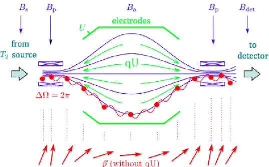
low energy electrons and last the Main spectrometer [19]. The Main spectrometer is used as an energy filter for the electrons working with high precision. The Main Spectrometer is a Magnetic Adiabatic Collimation Filter combined with an Electrostatic Filter (short MAC-E Filter). In Figure 2.2 it is shown how it works.

The gradient of the magnetic field collimates the momenta of the electrons in axial direction. The electric field’s task is to reflect electrons with a kinetic energy lower than the energy of the electric field qU, q denoting the charge and U the voltage of the high voltage system. The energy resolution of the MAC-E filter is:

∆E Ee

= Ba

Bp

= 3·10⁻⁴T

6T (2.2)

Bs is denoting the magnetic field in the analyzing plane wehereasBp is the maximal magnetic field generated by the pinch magnets. For energies of the electron around the endpoint of the spectrumEe = 18.6keV the Main spectrometer gives a resolution of ∆E = 0.93eV.

2.2 The Detector Section

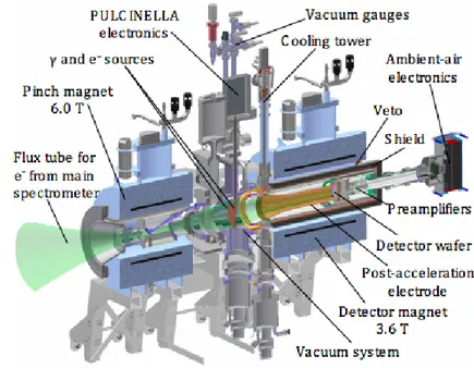
The Detector Section is set up at the end of the whole experimental setup. A schematic overview of how it is built can be seen in Figure 2.3 . It encompasses the silicon based pin-diode detector, or Focal Plane Detector (FPD) and a post acceleration electrode. The FPD has a radius of 4.5 m and is divided into 148 pixels. Each pixel has an area of 44mm². If an electron passed the potential of the Main Spectrometer, it is then detected in the FPD. Scanning the energy spectrum of the electron using different potentials in the Main Spectrometer allows to count electrons with an energy higher then the potential in the Main Spectrometer. Thus it is possible to measure an integral energy spectrum of the beta decay.

2.3 The TRISTAN Project

The TRISTAN group at the KATRIN experiment, with TRISTAN being short for TRitium Investigation of STerile to Active Neutrino mixing, aims to realize a tech- nical solution for the search of keV sterile neutrinos with KATRIN. It allows to investigate a mass range of the sterile mass eigenstatem4 in a range between 0 keV

(18)

Figure 2.2: The working principle of the MAC-E Filter used in the KATRIN experiment. Electrons, that get into the spectrometer, a guided along the magnetic field lines into the middle of the Main Spectrometer, reffered to as the analyzing plane. In the middle of the Main Spectrometer the electrostatic potential has its maximum, such that only electrons with high enough axial momenta are able to get to the detector.

and 18.6 keV [23]. Since this requires a measurement of the total beta decay energy spectrum, the electron rate at the detector needs to be increased by a factor of 10⁸. The TRISTAN group considers a two-stage approach. In the first stage, the Pre- KATRIN stage, the aim is to improve current laboratory limits after some days of measurements. To allow the measuring of the whole beta-spectrum, the spectrometer’s potential needs to be lower than 1kV. Additionally, the source of the tritium source needs to reduced by a factor of 10⁵, due to the fact that the FPD only allows a count rate of 100 kilo counts per secons. In the Post-KATRIN stage, the aim is to measure mixing angles below sin²θ = 10⁻⁶. Therefore, the whole strength of the source is needed. This implies a major modification of the experimental setup at KATRIN, especially in the Detector section, where a detector is required which will be able to handle the full rate of incoming electrons. There currently is work going on concerning the development of a Post-KATRIN detector. The TRISTAN group

(19)

Figure 2.3: Schematic overview of the Detector Section set up at the end of KA- TRIN’s experimental setup. The Main Spectrometer is on the left side of the shown setup.

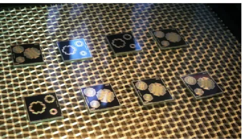
collaborates with the HalbLeiter LaborMunich (HLL) and the Lawrence Berkeley National Laboratory (LBNL), working on a prototype of a new pn-type silicon drift detector [24]. Each of those prototype detectros consists of seven hexagonal pixels.

Each of these pixels has a small read-out contact in the center. Several drift rings are positioned around the read-out contact. A picture of the detector prototypes can be seen in Figure 2.4.

(20)

Figure 2.4: Picture of the detector prototypes for the TRISTAN project produced at the HLL. Each chip contains seven pixels. The designs differ in size and the number of drift rings.

(21)

Chapter 3 Development of an

energy-dependent Final State Distribution

3.1 Introduction

As described in chapter one regarding the physics of active and sterile neutrinos, in the search for sterile neutrinos using experiments based on the nuclear β decay of tritium molecules (or isotopologes) the whole spectrum needs to be analysed, not only the endpoint, as in the measurement of the neutrino mass. The differential decay rate of the spectrum is given by

dΓ

dE =X

f

Pf·C·F(Z, E)·p·Etot·(E0−E−Ef)·q

Θ(E0−E−Ef −mν)·((E0−E−Ef)²−m²_ν)) (3.1)

withEf being the energy of the remaining orbital electron in the daughter molecule and Pf the corresponding probability, that the orbital electron will end up in this state after the dacay. The probability distribution for each state, that the electron can have in the daughter molecule, is called the Final State Distribution (FSD). So far, the FSD has only be calculated for the case of theβ electrons having an energy of 18.6 keV, thus for analysing the endpoint of the spectrum. Since the impact of

(22)

sterile neutrinos on the spectrum is way beyond the endpoint, an energy-dependent FSD is needed. The aim of this work is, to develop a simplified model describing the bahaviour of the FSD forβ energies below the endpoint, down to 12 keVβelectrons.

First, the theoretical background needed to develop that model will be discussed.

The theoretical calculations are based on the Sudden approximation, used to handle the evaluation of the matrix element. The derivation of the matrix element will be done by the Lippmann Schwinger ansatz [4], ending up in a zeroth order transition matrix element, that is independent on the recoil momentum of the escaping beta electron. The initial and final state in the matrix element are the wavefunctions of the T2 molecule and the daughter molecule ³HeT⁺. To get them, the Schr¨odinger equation needs to be solved. Therefore the Born-Oppenheimer approximation is used, to separate the molecular Schr¨odinger equation into a electronic and a nuclear part. Solving the nuclear part of the coupled equations requires numerical methods.

Therefore the technique of expanding wavefunctions in terms of B-Splines will be explained. Following the theoretical framework, a description of the four main parts of the FSD will be given. After that, the focus will lie on the development of an simplified energy-dependent description of the first two parts - the groundstate and the first five electronically excited states. In the conclusion we will have a look at the differences to the use of old models in the beta decay spectrum containing sterile neutrinos.

3.2 The Sudden Approximation

To get the Final State Probability distribution, the transition probabilities from an initial state (in this case the T2 molecule) to a final state (HeT⁺) need to be calculated. Since the calculations of the matrix elements can get pretty complicated, the first step is to simplify those using the so called Sudden approximation [9].

Quantum mechanical systems are in general described by a Hamiltonian H. If this system goes through a change (i.e. a nuclear β decay), the Hamiltonian changes as well as the properties of the system. To treat this change in a simplified manner, the sudden approximation is applied. Start with a Hamiltonian H0 describing a quantum mechanical system, before a sudden perturbation to the system happens at timet= 0 to a system described by the HamiltonianH1. Both Hamiltonians are assumed to be independent of time. Before the change, for t < 0, the Schr¨odinger equation for the system is:

H0ψk =E_k⁽⁰⁾ψk (3.2)

(23)

with E_k⁽⁰⁾ and ψk being the eigenvalues and eigenfunctions of the Hamiltonian H0. The eigenfunctions of this system are assumed to form a complete, orthonormal set ψk. The solution to the time-dependent Schr¨odinger equation

i¯h ∂

∂tψk =Hψ (3.3)

is then described by the expansion ψ(t) =X

k

akψke^−iE^k⁽⁰⁾^t/¯^h (3.4) The summation goes through all eigenfunctions from the complete and orthonormal setψk. The coefficientsakshall be independent of time. Under the assumption of the eigenfunctions being normalised to unity, the absolute square of those coefficients may be interpreted as the probability to find the system in the state |ψki. At time t= 0 the system gets perturbed and the Hamiltonian suddenly changes toH1. The time-independent Schr¨odinger equation then becomes:

H₁φn =E_k⁽¹⁾φn (3.5)

with the time-dependent solution being ψ(t) =X

n

cnφne^−iEⁿ⁽⁰⁾^t/¯^h (3.6) again with a summation over the set of all eigenfunctions with time-independent coefficients cn. Since the time-dependent Schr¨odinger equation is of first order in time, the wavefunction ψ(t) must be continous in time t. This continuity has to hold during the sudden change of the Hamiltonian as well. Thus at the time of the sudden change, t=0, the condition

X

k

ak|ψki=X

n

cn|φni (3.7)

has to hold. By multiplying this eqaution by hφn| and using hφn |φmi = δm,n the time-independent coefficientscn are given by:

cn=X

k

akhφn |ψki (3.8)

(24)

Under the assumption, that the Hamiltonian of the system changes instantaneously, this condition for the coefficients is exact. Since such a change usually happens during a time interval of finite length τ, the Hamiltonian H₀ first changes to Hi, with Hi being valid in the interval 0 < t < τ, and then, for t > τ to H1. The time-independent Schr¨odinger equation for the Hamiltonian Hi is then, as usual:

Hiχl =E_l⁽ⁱ⁾χl (3.9)

and the time-dependent solutionψ(t) =P

lblχle^−iE^l⁽ⁱ⁾^t/¯^h. Since the condition of the wavefunction remaining continous during the perturbation still holds, at time t=0 the equation

X

k

akψk=X

l

blχl (3.10)

holds, which yields the the condition for the coefficients bl: bl =X

k

akhχl|ψki (3.11)

At the timet =τ the wavefunction has to stay continous as well, thus yielding:

X

l

blχle^−iE⁽ⁱ⁾^l ^{τ /¯}^h =X

n

cnφne^−iEⁿ⁽¹⁾^{τ /¯}^h (3.12) Pluggin in the solution for the coefficientsbl from before, one gets for the cn:

cn=X

k

X

l

akhφn|χli hχl|ψkie^i(Eⁿ⁽⁰⁾^−E⁽ⁱ⁾^l ^{)τ /¯}^h (3.13) For an instantaneous change of the system with τ = 0 the above equation for the coefficientscngets the known form. Forτ 6= 0, the difference lies in the exponentials.

If this time duration τ is small compared to ^¯^h

|E_n⁽⁰⁾−E⁽ⁱ⁾_l |, which means (En⁽⁰⁾−E_l⁽ⁱ⁾)τ

¯

h 1 (3.14)

the change of the wavefunction in the interval 0< t < τ is small and can thus be neglected. The sudden approximation is then to set τ = 0. In the following, the transition probability for the decay of a tritium nucleus in a tritium molecule will be derived using the Lippmann-Schwinger expansion. The total probability amplitude will be written as the sum of the zeroth, the first etc. order amplitudes with the zeroth order probability amplitude corresponding to the transition probability within the sudden approximation.

(25)

3.3 Derivation of the transition probability

The derivation of the transition probability is described in [4] and will be shown in detail now. Consider to start with the process

RT →RHe⁺+e⁻+ ¯ν (3.15)

The Hamiltonian for the whole system H = Hi,f +Vi,f is divided into the part Hi,f describing the molecular system and a single lepton either in its inital or final state andVi,f describing the interaction between them. Hi,f can be seen as the free Hamiltonian and Vi,f as a small perturbation. The interaction term can be split in the following way:

Vi,f =Ui,f +Wi,f (3.16)

Here Ui,f stands for the coulombian interaction and Wi,f for the weak interaction causing the dacay. The transition probability of a molecule RT with a rest R to a molecule RHe⁺ after beta-decay is described dy:

|Tf i |²=| hf|Wi|ii |²=| hψf|Wi|Φii |² (3.17) Tf i is the transition matrix element, hψf| is the final eigenstate of the Hamiltonian H and|Φiiis the eigenstate of the free HamiltonianHi describing the initial motion of the RT molecule. Wi is the operator describing the weak interaction process.

Now the final eigenstate hψf| of the Hamiltonian H can be expanded using the Lippmann-Schwinger ansatz:

hψf|=hΦf|+hΦf|Vf(E−Hf +i)⁻¹+... (3.18) where (E−Hf +i)⁻¹ is the free Greens function and hΦf| is the eigenstate of the free Hamiltonian Hf. With Vf = Uf the transition matrix element can be written in the following way:

Tf i =hψf|Wi|Φii=hΦf|Wi|Φii+hΦf|Uf(E−Hf +i)⁻¹Wi|Φii+...= (3.19) hΦf|Wi|Φii+hΦf|Uf(E−Hf +i)⁻¹|Φii+...= (3.20) T_{f i}⁽⁰⁾+T_{f i}⁽¹⁾+... (3.21)

(26)

Here Φi,f are the initial and final eigenvectors of the free Hamiltonian Hi,f. In the above equation higher order terms are neglegted due to the smallness of the weak coupling constant. For the purposes of this work, only the zeroth order transition matrix element is of interest.

3.3.1 Evaluation of T_{f i}⁽⁰⁾

The process

RT →RHe⁺+e⁻+ ¯ν (3.22)

represents a decay of one particle into three final particles. According to field theory, such processes can be described as a scattering process. The emission of a particle corresponds to the absorption of an antiparticle with opposite energy. Thus the decay process can be described by a more symmetrical

RT +ν →RHe⁺+e (3.23)

The free Hamiltonian for the initial state of the molecule can be written as

Hi =HRT +Hν (3.24)

whereas the free Hamiltonian for the final state is

Hf =HRHe⁺ +Hβ (3.25)

The Hamiltonians can be further divided into

Hf,i=T^c.m.+H^mol+H^nuc (3.26) where T^c.m. describes the center of mass motion of the molecule, H^mol describes the Coulombian Hamiltonian terms and H^nuc the internal motion of the nucleons.