Parameters in Laryngeal High-Speed Videoendoscopy

applied sciences

Article

Influence of Analyzed Sequence Length on

Parameters in Laryngeal High-Speed Videoendoscopy

Patrick Schlegel

* , Marion Semmler

, Melda Kunduk

, Michael Döllinger

, Christopher Bohr

and Anne Schützenberger

1

Department of Otorhinolaryngology, Division of Phoniatrics and Pediatric Audiology, University Hospital Erlangen, Friedrich-Alexander-University Erlangen-Nürnberg, 91054 Erlangen, Germany;

Marion.Semmler@uk-erlangen.de (M.S.); Michael.Doellinger@uk-erlangen.de (M.D.);

Anne.Schuetzenberger@uk-erlangen.de (A.S.)

2

Department of Communication Sciences and Disorders, Louisiana State University, Baton Rouge, LA 70803, USA; mkunduk@gmail.com

3

Department of Otorhinolaryngology, University Hospital Regensburg, 93053 Regensburg, Germany;

Christopher.Bohr@klinik.uni-regensburg.de

* Correspondence: Patrick.Schlegel@uk-erlangen.de; Tel.: +49-09131-85-33815

Received: 23 October 2018; Accepted: 13 December 2018; Published: 18 December 2018

Abstract: Laryngeal high-speed videoendoscopy (HSV) allows objective quantification of vocal fold vibratory characteristics. However, it is unknown how the analyzed sequence length affects some of the computed parameters. To examine if varying sequence lengths influence parameter calculation, 20 HSV recordings of healthy females during sustained phonation were investigated. The clinical prevalent Photron Fastcam MC2 camera with a frame rate of 4000 fps and a spatial resolution of 512 × 256 pixels was used to collect HSV data. The glottal area waveform (GAW), describing the increase and decrease of the area between the vocal folds during phonation, was extracted.

Based on the GAW, 16 perturbation parameters were computed for sequences of 5, 10, 20, 50 and 100 consecutive cycles. Statistical analysis was performed using SPSS Statistics, version 21. Only three parameters (18.8%) were statistically significantly influenced by changing sequence lengths. Of these parameters, one changed until 10 cycles were reached, one until 20 cycles were reached and one, namely Amplitude Variability Index (AVI), changed between almost all groups of different sequence lengths. Moreover, visually observable, but not statistically significant, changes within parameters were observed. These changes were often most prominent between shorter sequence lengths. Hence, we suggest using a minimum sequence length of at least 20 cycles and discarding the parameter AVI.

Keywords: high-speed videoendoscopy; glottal area waveform; sequence length; parameters; diagnosis

1. Introduction

The vocal folds are located in the larynx and produce the source signal for voice and speech.

They start vibrating when the tracheal airflow, coming from the lungs, sets them in motion. During vibration of the vocal folds this airflow is interrupted, resulting in audible sound. After passing the vocal folds, the airflow is further modulated by tongue and lips, producing voice and speech in the process [1,2]. The vocal folds vibrate in varying frequency. Upper range of females’ fundamental frequency (F0) were reported to range from 250 Hz [3,4] to 1000 Hz [5]. During singing even higher frequencies of up to 1568 Hz were reported [6].

Vocal fold vibratory patterns can be investigated using several imaging techniques.

Videostroboscopy (VS) produces an illusory slow motion by relying on the assumption of the periodic nature of vocal fold vibration. With short strobe light flashes, single images from consecutive oscillation

Appl. Sci.2018,8, 2666; doi:10.3390/app8122666 www.mdpi.com/journal/applsci

Appl. Sci.2018,8, 2666 2 of 17

cycles are recorded with a small delay to the previous cycle. These images are then assembled to artificial glottal cycles. However, since VS presents only an artificial slow motion, even subtle variation in periodicity of the vocal fold vibration can result in completely distorted or unrealistic image sequences [7]. Another technique in use is videokymography (VK), which, in contrast to VS, records the vocal fold oscillation at frame rates of about 7000 to 8000 Hz [7–10], which is distinctly higher than the vocal folds vibration frequency, but can only scan a single line across the glottis [7]. With high-speed videoendoscopy (HSV), the whole glottis is recorded using a high-speed camera [7,11] with frame rates of currently about 4000 Hz in clinical applications [12–15]. Hence, HSV overcomes the limitations of VS and VK and combines the advantages of both techniques [7,11].

Since the introduction of HSV to laryngeal examination, numbers of different studies using HSV have been published [16–21]. Also, HSV is no longer reserved for scientific use only; the clinical applicability of HSV was tested recently on a larger scale in comparison with VS Ratings of all vibratory features which showed changes between VS and HSV and it was concluded that HSV could enable important refinements in diagnosis and management of vocal fold pathology [22]. As HSV is superior to alternative procedures such as VS and VK [7,14,23], it possesses the potential to replace VS [11], the longtime “gold standard” and widely used technique of laryngeal examination [24–26]. However, HSV systems are expensive and these high costs are considered as the most prohibitive factor for the widespread clinical implementation of HSV [7].

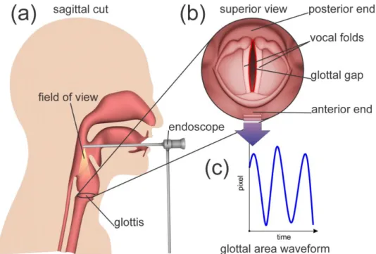
A typical clinical examination situation, as it is used for HSV using rigid endoscope, is illustrated in Figure 1. The vibration of the vocal folds is recorded from above [27]. From the recorded data, different features can be extracted. The most prominent and significant feature is the glottal area waveform (GAW). The GAW describes the area between the vocal folds, the “glottal area”, which opens and closes periodically during normal phonation. For each individual video frame, the glottal area is segmented and lined up in a function as shown in Figure 1b,c. The GAW is defined slightly differently in different works [28–31]. In this work, the GAW is defined as the function of the glottal area in pixels over frames. All parameters used in this work were calculated using this definition of the GAW.

Appl. Sci. 2018, 8, x FOR PEER REVIEW 2 of 18

Vocal fold vibratory patterns can be investigated using several imaging techniques.

Videostroboscopy (VS) produces an illusory slow motion by relying on the assumption of the periodic nature of vocal fold vibration. With short strobe light flashes, single images from consecutive oscillation cycles are recorded with a small delay to the previous cycle. These images are then assembled to artificial glottal cycles. However, since VS presents only an artificial slow motion, even subtle variation in periodicity of the vocal fold vibration can result in completely distorted or unrealistic image sequences [7]. Another technique in use is videokymography (VK), which, in contrast to VS, records the vocal fold oscillation at frame rates of about 7000 to 8000 Hz [7–10], which is distinctly higher than the vocal folds vibration frequency, but can only scan a single line across the glottis [7]. With high-speed videoendoscopy (HSV), the whole glottis is recorded using a high-speed camera [7,11] with frame rates of currently about 4000 Hz in clinical applications [12–15]. Hence, HSV overcomes the limitations of VS and VK and combines the advantages of both techniques [7,11].

Since the introduction of HSV to laryngeal examination, numbers of different studies using HSV have been published [16–21]. Also, HSV is no longer reserved for scientific use only; the clinical applicability of HSV was tested recently on a larger scale in comparison with VS Ratings of all vibratory features which showed changes between VS and HSV and it was concluded that HSV could enable important refinements in diagnosis and management of vocal fold pathology [22]. As HSV is superior to alternative procedures such as VS and VK [7,14,23], it possesses the potential to replace VS [11], the longtime “gold standard” and widely used technique of laryngeal examination [24–26].

However, HSV systems are expensive and these high costs are considered as the most prohibitive factor for the widespread clinical implementation of HSV [7].

A typical clinical examination situation, as it is used for HSV using rigid endoscope, is illustrated in Figure 1. The vibration of the vocal folds is recorded from above [27]. From the recorded data, different features can be extracted. The most prominent and significant feature is the glottal area waveform (GAW). The GAW describes the area between the vocal folds, the “glottal area”, which opens and closes periodically during normal phonation. For each individual video frame, the glottal area is segmented and lined up in a function as shown in Figure 1b,c. The GAW is defined slightly differently in different works [28–31]. In this work, the GAW is defined as the function of the glottal area in pixels over frames. All parameters used in this work were calculated using this definition of the GAW.

Figure 1. (a) Recording of the vocal fold oscillations via a rigid endoscope being attached to a high-

speed camera. (b) Superior view of the vocal folds as seen with the endoscope. (c) Computed glottal area waveform (GAW): amount of registered pixels in the glottis over time.

Figure 1. (a) Recording of the vocal fold oscillations via a rigid endoscope being attached to a high-speed camera. (b) Superior view of the vocal folds as seen with the endoscope. (c) Computed glottal area waveform (GAW): amount of registered pixels in the glottis over time.

Even though HSV, sometimes done in combination with recording of the audio signal [32,33], is a

powerful method for examining the phonation process [7], the objective parameters obtained from

Appl. Sci.2018,8, 2666 3 of 17

both can be influenced by different factors [34–38]. One of these factors is the recording frame rate, which was already investigated for acoustic and GAW signals. For acoustic measures, a sampling frequency of at least 26 kHz was suggested to avoid the introduction of errors [34]. For GAW signals it is reported that up to 90% of parameters were affected by the changes in the frame rate [35].

That study suggested that normative parameter values based on the recording frame rate should be determined and a recording frequency of 4000 Hz seemed to be too low to register all details of vocal fold vibratory patterns. Still, the application of recording frame rates of 4000 Hz in clinical studies was judged as justified, since the parameter changes between 4000 Hz and 15,000 Hz were relatively small for glottal dynamic characteristics and glottal perturbation characteristics. For acoustic signals, the stability of perturbation measures was investigated with deviating results [36–38]. Scherer et al.

suggested a minimal sequence length in the order of 100 cycles for the calculation of stable perturbation measures in the acoustic signal [36]. Karnell et al. found that frequency and amplitude perturbation measures (APM) were not in agreement for three different analysis systems, even for 110 consecutive cycles [37]. Another investigation was done for the electroglottographic (EGG) signal, which describes the electrical impedance between two electrodes placed on the left and right side of the larynx and changes with vocal fold vibration. The influence of different sequence lengths on EGG and audio was investigated and it was found that two of nine perturbation measures for the EGG signal and two of nine perturbation measures for the audio signal (although not the same measures) were affected by changing sequence lengths [38]. However, to the best of the authors’ knowledge, no studies exist examining the influence of the analyzed interval length especially for GAW parameters computed from HSV data.

In various studies, perturbation parameters are calculated for the GAW, and often the analyzed sequence length varies [39–42]. Moreover, the sequence lengths are often given in milliseconds [39,40];

hence the number of cycles ultimately used to calculate the perturbation measures may vary within these studies. To find out if and how this affects the comparability of these studies, the current work investigated the influence of a differing sequence length on 16 different perturbation parameters.

Specifically, period, amplitude and energy perturbation parameters were investigated. The aims of this work can be summarized in the following way:

1. Examine if varying sequence length affects GAW perturbation parameters.

2. Determine if there is a statistical change in parameters by varying sequence length.

3. Investigate the reason for the susceptibility of these parameters to a changing sequence length.

These goals are met by a systematic analysis of all 16 examined perturbation measures. A detailed discussion of the statistically significantly changes in parameters due to varying sequence length was given. The suggestion of the use of at least 20 cycles was given for future studies using HSV data.

2. Materials and Methods

Twenty endoscopically recorded HSV data from 20 healthy female subjects were investigated.

All recordings were chosen from our existing clinical database. Data collection and usage was approved by the ethic committee of the Medical School at Friedrich-Alexander-University Erlangen-Nürnberg (no. 290_13B). All subjects phonated the vowel /i/ at a comfortable pitch and loudness level during examination. All 20 videos chosen for this study had a comparatively good recording quality with visibility of the entire glottis and good brightness and contrast. The chosen videos were recorded by the clinically used Photron Fastcam MC2 with a spatial resolution of 512 × 256 pixels and a frame rate of 4000 fps. All chosen videos included at least 102 consecutive cycles of glottis closing and opening. The sequences of 100 cycles used for analysis ranged in length from 234.75 ms (427.11 Hz F0) to 426.50 ms (234.69 Hz F0). Therefore, with a sampling rate of 4000 Hz the Nyquist sampling criterion was more than satisfied with respect to GAW F0.

All recordings were segmented using a modified version of our in house developed software,

Glottis Analysis Tools (GAT–2018). This modified version was slightly adjusted to allow a smaller

Appl. Sci.2018,8, 2666 4 of 17

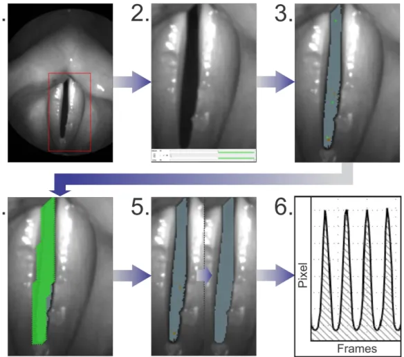
inter seed point distance and a more precise segmentation. The segmentation procedure is depicted in Figure 2 and was as follows:

1. A region of interest in the video was selected, which included full view of glottis.

2. An interval containing at least 102 cycles during constant phonation was selected. When selecting the intervals, care was taken to choose sections in which the glottis was completely visible and the field of view moved as little as possible.

3. For the initial pre-segmentation, seed points (green crosses in Figure 2(3,4)) were set and brightness thresholds were used. All pixels surrounding a seed point position including the pixel on the position itself are marked, if they are darker than the selected brightness thresholds.

4. Afterwards the seed points were substituted by a regular seed point grid. In the grid region every second pixel was marked with a seed point. The grid was created semi-automatically by using a seed point drawing tool.

5. The brightness thresholds were adjusted yielding the finalized brightness settings.

6. The total GAW (GAW

) was extracted for each recording.

Appl. Sci. 2018, 8, x FOR PEER REVIEW 4 of 18

All recordings were segmented using a modified version of our in house developed software, Glottis Analysis Tools (GAT–2018). This modified version was slightly adjusted to allow a smaller inter seed point distance and a more precise segmentation. The segmentation procedure is depicted in Figure 2 and was as follows:

1. A region of interest in the video was selected, which included full view of glottis.

2. An interval containing at least 102 cycles during constant phonation was selected. When selecting the intervals, care was taken to choose sections in which the glottis was completely visible and the field of view moved as little as possible.

3. For the initial pre-segmentation, seed points (green crosses in Figure 2.3.,2.4.) were set and brightness thresholds were used. All pixels surrounding a seed point position including the pixel on the position itself are marked, if they are darker than the selected brightness thresholds.

4. Afterwards the seed points were substituted by a regular seed point grid. In the grid region every second pixel was marked with a seed point. The grid was created semi-automatically by using a seed point drawing tool.

5. The brightness thresholds were adjusted yielding the finalized brightness settings.

6. The total GAW (GAW

) was extracted for each recording.

Figure 2. Illustration of the segmentation process: (1) Selection of the region of interest; (2) Selection of a time interval with constant phonation; (3) Rough pre-segmentation; (4) Applying a seed point grid; (5) Refinement of the brightness thresholds; (6) Extraction of the total GAW.

The segmentation was performed using regular grids of seed points (i.e., setting the seed points in an organized mesh, as it can be seen in Figure 2.4.). This segmentation style was chosen to ensure a more objective segmentation and minimalize errors by missed small sections of the glottal area.

However, this method of segmentation is only applicable for recordings with sufficiently good Figure 2. Illustration of the segmentation process: (1) Selection of the region of interest; (2) Selection of a time interval with constant phonation; (3) Rough pre-segmentation; (4) Applying a seed point grid;

(5) Refinement of the brightness thresholds; (6) Extraction of the total GAW.

The segmentation was performed using regular grids of seed points (i.e., setting the seed points in an organized mesh, as it can be seen in Figure 2(4)). This segmentation style was chosen to ensure a more objective segmentation and minimalize errors by missed small sections of the glottal area.

However, this method of segmentation is only applicable for recordings with sufficiently good contrast

and clearly visible boundaries of the glottal area. Altogether 20 GAW

signals were calculated.

Appl. Sci.2018,8, 2666 5 of 17

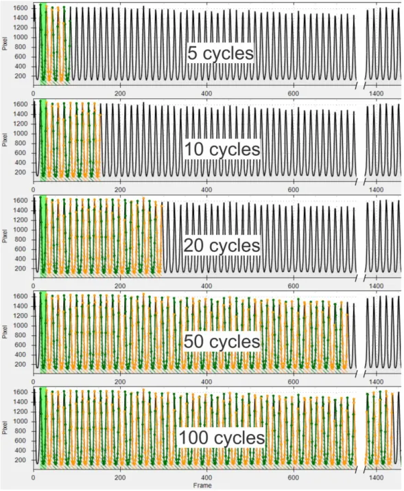
Maximum based cycle detection was chosen to determine the cycles of the GAW

signals.

Each cycle starts at a significant local maximum and ends one frame before the next one. Beginning with the second detected cycle, as Figure 3 illustrates, for each GAW 5, 10, 20, 50 and 100 consecutive cycles were selected for parameter computation, yielding five “cycle sets” per GAW. Since significant influences on the parameter calculation by frequency shifts in the phonation or field of view movements become more likely with growing recording length [43], no longer cycle sets were chosen. Furthermore, greater numbers of cycles will add more analysis time and would not be feasible in a clinical setting. From the cycle sets, 16 different perturbation parameters were calculated. All 16 parameters, their origin and a brief description are summarized in Table 1.

Appl. Sci. 2018, 8, x FOR PEER REVIEW 5 of 18

contrast and clearly visible boundaries of the glottal area. Altogether 20 GAW

signals were calculated.

Maximum based cycle detection was chosen to determine the cycles of the GAW

signals. Each cycle starts at a significant local maximum and ends one frame before the next one. Beginning with the second detected cycle, as Figure 3 illustrates, for each GAW 5, 10, 20, 50 and 100 consecutive cycles were selected for parameter computation, yielding five “cycle sets” per GAW. Since significant influences on the parameter calculation by frequency shifts in the phonation or field of view movements become more likely with growing recording length [43], no longer cycle sets were chosen.

Furthermore, greater numbers of cycles will add more analysis time and would not be feasible in a clinical setting. From the cycle sets, 16 different perturbation parameters were calculated. All 16 parameters, their origin and a brief description are summarized in Table 1.

Figure 3. For each segmented GAW 5 sets of consecutive cycles are chosen for analysis.

Figure 3. For each segmented GAW 5 sets of consecutive cycles are chosen for analysis.

Appl. Sci.2018,8, 2666 6 of 17

Table 1. Information for all investigated parameters.

Parameter (Unit) and Reference Abbreviation Parameter Description Period Perturbation Measures (PPM)

Mean Jitter(ms) [44] MJit Mean deviation in duration between cycle pairs Jitter(%) (a.u.) [44] Jit(%) Normalized mean deviation in duration between

cycle pairs

Jitter Factor(a.u.) [45] JitFac Normalized mean deviation of reciprocal in duration between cycle pairs

Jitter Ratio(a.u.) [46] JitRat Normalized mean deviation in duration between cycle pairs

Period Perturbation Quotient-3%

(a.u.) [47]¹ PPQ3

Difference in cycle lengths based on the mean difference between each inner cycle and its neighboring cycles

Period Perturbation Factor(a.u.) [47]¹ PPF Mean normalized deviation in duration between cycle pairs

Relative Average PerturbationBielamowicz

(a.u.) [48] RAP_B Difference in cycle lengths based on the difference between each inner cycle and its neighboring cycles Relative Average Perturbation_Koike

(a.u.) [49] RAP_K

Normalized difference in cycle lengths based on the difference between each inner cycle and its neighboring cycles

Period Variability Index(a.u.) [50] PVI Normalized mean quadratic deviation in duration between each cycle and an average cycle

Amplitude Perturbation Measures (APM)

Mean Shimmer(decibel) [44] MShim Mean logarithmized deviation in dynamic range² between cycle pairs

Shimmer (%)(dB/log10(pixel)) [51] Shim(%) Normalized mean logarithmized deviation in dynamic range between cycle pairs

Amplitude Perturbation Quotient-3%

(a.u.) [47] APQ3

Difference in dynamic range based on the mean difference between each inner cycle and its neighboring cycles

Amplitude Perturbation Factor(a.u.) [47] APF Mean normalized deviation in dynamic range between cycle pairs

Amplitude Variability Index(decibel) [50] AVI

Logarithmized normalized mean quadratic deviation in dynamic range between each cycle and an average cycle

Energy Perturbation Measures (EPM)

Energy Perturbation Quotient-3%(a.u.) [47] EPQ3 Difference in energy based on the mean difference between each inner cycle and its neighboring cycles Energy Perturbation Factor(a.u.) [47] EPF Mean normalized deviation in energy between

cycle pairs

1In the source material one formula is given as “Perturbation Quotient” and one as “Perturbation Factor”. The different types of Perturbation Quotients and Factors in this work were calculated by inserting cycle lengths, dynamic ranges and cycle energies in these original formulas for, in case of thePerturbation Quotient, k = 3.²The “dynamic range”

is defined as the maximum of the glottal area in one cycle minus the minimum of the glottal area in the same cycle.

Each parameter was computed for each of the five cycle sets for each of the 20 GAW

signals.

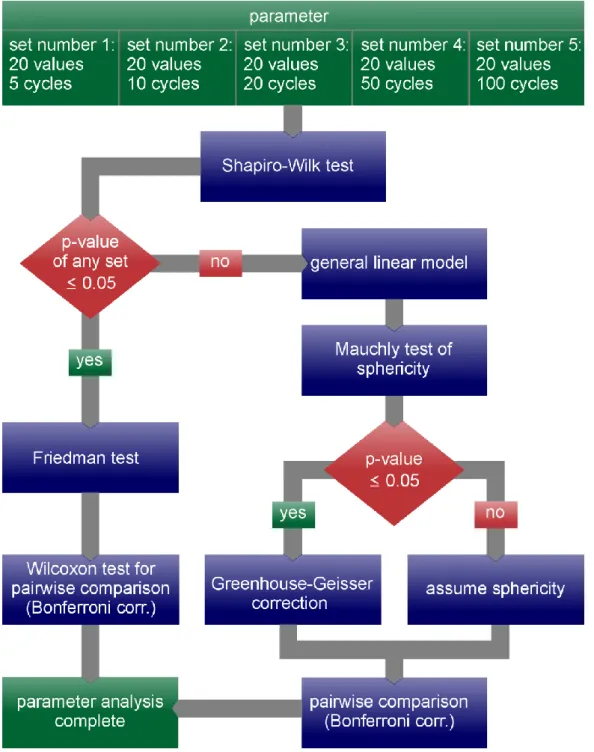
All values of one parameter calculated from one cycle set were grouped together resulting in five sets of 20 values each for every parameter. Each set of values referring to a sequence length from 5 to 100 cycles. These five sets were compared with each other for every parameter. Therefore, pairwise tests for connected samples using SPSS Statistics version 21 were performed. For each test the H

Hypothesis was rejected if the p-value was equal or less than 0.05. For the general linear model (GLM), repeated measures with five within-subject variables (i.e., the five sequence lengths) were chosen.

The default setting of a saturated model with a Type III sum of squares was retained. We applied

Bonferroni correction to pairwise comparisons (see Figure 4) by multiplying p-values of post hoc tests

by five. The p-values were clipped at 1. The workflow of the entire statistical analysis is shown in

Figure 4.

Appl. Sci.2018,8, 2666 7 of 17

Appl. Sci. 2018, 8, x FOR PEER REVIEW 7 of 18

cycles. These five sets were compared with each other for every parameter. Therefore, pairwise tests for connected samples using SPSS Statistics version 21 were performed. For each test the H

Hypothesis was rejected if the p-value was equal or less than 0.05. For the general linear model (GLM), repeated measures with five within-subject variables (i.e., the five sequence lengths) were chosen. The default setting of a saturated model with a Type III sum of squares was retained. We applied Bonferroni correction to pairwise comparisons (see Figure 4) by multiplying p-values of post hoc tests by five. The p-values were clipped at 1. The workflow of the entire statistical analysis is shown in Figure 4.

Figure 4. For each parameter, five sets of values for different sequence lengths were calculated. The

sets range from 5 consecutive cycles (set number 1) to 100 consecutive cycles (set number 5) and contain 20 values each. Then the depicted statistical analysis workflow was performed for each parameter.

Figure 4. For each parameter, five sets of values for different sequence lengths were calculated. The sets range from 5 consecutive cycles (set number 1) to 100 consecutive cycles (set number 5) and contain 20 values each. Then the depicted statistical analysis workflow was performed for each parameter.

3. Results

Statistical analysis revealed a statistically significant change in three out of 16 examined parameters for different sequence lengths. The significantly changing parameters were Amplitude Variability Index (AVI) (p < 0.001), Relative Average Perturbation

(RAP

) (p < 0.001) and Amplitude Perturbation Quotient-3% (APQ3) (p = 0.017).

Post hoc tests disclosed that AVI changed between almost all different pairings of sequence

lengths. The only not statistically significantly different pairings were between 5 and 10 and between

10 and 20 cycles. RAP

changed statistically significantly until 20 consecutive cycles were reached and

Appl. Sci.2018,8, 2666 8 of 17

APQ3 changed statistically significantly until 10 consecutive cycles were reached. Statistical p-values of all parameters can be seen in Table S1 in the supplementary information.

This table contains the p-values for all Friedman and GLM tests and all performed post hoc tests.

Additionally, descriptive values, i.e., group means, standard deviation, maximum and minimum values for period, amplitude and energy perturbation parameters for all sequence lengths are represented in Appendix A in Tables A1–A3. Last in Table 2 a summary of all observed statistically significant changes and also systematic in- or decreases for all parameters is given.

Table 2. Statistically significant parameter changes and observed systematic in- or decreases.

Statistically Significant Changes

Parameter Overall Test Significance Significantly Different Cycle Pairings

RAP

p < 0.001 5–10, 5–20, 5–50, 5–100, 10–20

APQ3 p = 0.017 5–10, 5–20, 5–50

AVI p < 0.001 5–20, 5–50, 5-100, 10–50, 10–100, 20–50, 20–100, 50–100 Systematic in- or decreases

Parameter Mean value Standard deviation Max value Min value Period Perturbation Measures (PPM)

MJit

100

10

Jit(%)

50

20

JitFac

50

20

JitRat

50

20

PPQ3

50

100

20

PPF

50

20

RAP

RAP

50

20

PVI

20

Amplitude Perturbation Measures (APM)

MShim

10

100

100

Shim(%)

10

100

100

APQ3

100

100

100

APF

10

100

100

AVI

50

Energy Perturbation Measures (EPM)

EPQ3

50

100

20

10

EPF

100

20

1 Ôx Indicates that the calculated descriptive value increased monotonically until x consecutive cycles were reached.²Ôx Indicates that the calculated descriptive value decreased monotonically until x consecutive cycles were reached.

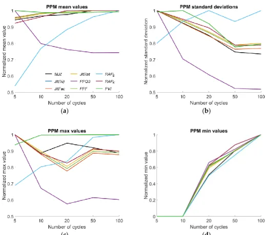
In addition to the statistically significant changes, visual subjectively observable trends were

found. As depicted in Figure 5, for the Period Perturbation Measures (PPM) the descriptive values

i.e., group mean, standard deviation, maximum and minimum of most parameters increased or

decreased consistently up to certain sequence lengths. To give a visual impression for parameter

behavior in this figure, the descriptive values were normalized to their maximum values for a better

comparability. The same standardization was applied to the data depicted in Figures 6 and 7. Detailed

information of observed systematic increases or decreases in descriptive values for all parameters is

given in Table 2.

Appl. Sci.2018,8, 2666 9 of 17

Appl. Sci. 2018, 8, x FOR PEER REVIEW 9 of 18

behavior in this figure, the descriptive values were normalized to their maximum values for a better comparability. The same standardization was applied to the data depicted in Figures 6 and 7.

Detailed information of observed systematic increases or decreases in descriptive values for all parameters is given in Table 2.

(a) (b)

(c) (d)

Figure 5. Period Perturbation measures (PPM): (a) normalized group means, (b) standard deviation, (c) maximum value, (d) minimum value.

(a) (b)

Figure 5. Period Perturbation measures (PPM): (a) normalized group means, (b) standard deviation, (c) maximum value, (d) minimum value.

Appl. Sci. 2018, 8, x FOR PEER REVIEW 9 of 18

behavior in this figure, the descriptive values were normalized to their maximum values for a better comparability. The same standardization was applied to the data depicted in Figures 6 and 7.

Detailed information of observed systematic increases or decreases in descriptive values for all parameters is given in Table 2.

(a) (b)

(c) (d)

Figure 5. Period Perturbation measures (PPM): (a) normalized group means, (b) standard deviation, (c) maximum value, (d) minimum value.

(a) (b)

Appl. Sci. 2018, 8, x FOR PEER REVIEW 10 of 18

(c) (d)

Figure 6. Amplitude Perturbation measures (APM) with exception of Amplitude Variability Index (AVI):

(a) normalized group means, (b) standard deviation, (c) maximum value, (d) minimum value.

(a) (b)

(c) (d)

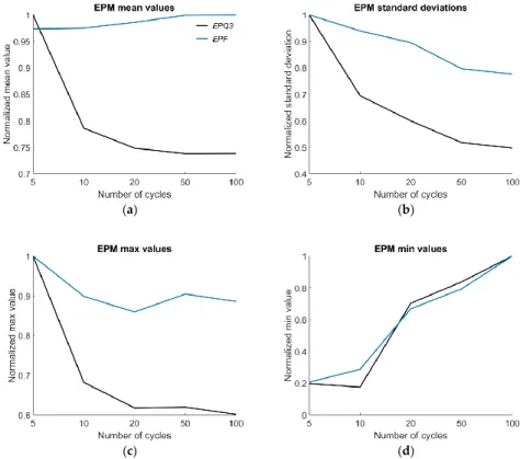
Figure 7. Energy Perturbation measures (EPM): (a) normalized group means, (b) standard deviation, (c) maximum value, (d) minimum value.

The descriptive values for amplitude perturbation are depicted in Figure 6. The

excluded from this figure since it can become negative and was hence not suitable for relative comparison. In other words, if AVI would be normalized in the same way as the other parameters, it would map to a number space outside the 0 to 1 interval.

Figure 6. Amplitude Perturbation measures (APM) with exception of Amplitude Variability Index (AVI):

(a) normalized group means, (b) standard deviation, (c) maximum value, (d) minimum value.

Appl. Sci.2018,8, 2666 10 of 17

Appl. Sci. 2018, 8, x FOR PEER REVIEW 10 of 18

(c) (d)

Figure 6. Amplitude Perturbation measures (APM) with exception of Amplitude Variability Index (AVI):

(a) normalized group means, (b) standard deviation, (c) maximum value, (d) minimum value.

(a) (b)

(c) (d)

Figure 7. Energy Perturbation measures (EPM): (a) normalized group means, (b) standard deviation, (c) maximum value, (d) minimum value.

The descriptive values for amplitude perturbation are depicted in Figure 6. The AVI was excluded from this figure since it can become negative and was hence not suitable for relative comparison. In other words, if AVI would be normalized in the same way as the other parameters, it would map to a number space outside the 0 to 1 interval.

Figure 7. Energy Perturbation measures (EPM): (a) normalized group means, (b) standard deviation, (c) maximum value, (d) minimum value.

The descriptive values for amplitude perturbation are depicted in Figure 6. The AVI was excluded from this figure since it can become negative and was hence not suitable for relative comparison.

In other words, if AVI would be normalized in the same way as the other parameters, it would map to a number space outside the 0 to 1 interval.

In Figure 7, the descriptive values for all examined Energy Perturbation measures (EPM) are plotted.

4. Discussion

The segmented glottal area can be affected by changing illumination, camera movement and larynx movement itself, which influences the calculated dynamic ranges (maximum minus minimum of the glottal area in 1 cycle). Hence the dynamic ranges may increase or decrease over time for some segments of the signal. This also explains the statistically significant change in AVI between all groups of sequence lengths in contrast to the other unaffected APM. AVI does not compare the dynamic ranges of consecutive cycles in pairs but instead compares each single dynamic range to an average dynamic range calculated for all cycles (see Table 1). For this reason, AVI is more sensitive to long term changes in the signal. As the dynamic ranges continue to increase or decrease in the signal course, the distance between the average dynamic range and the dynamic ranges of each cycle increases with the signal length, which in turn affects the AVI. As opposed to this, the influence of such long-term effects on perturbation parameters comparing only neighboring cycles does not grow with the sequence length. Analogous to AVI also Period Variability Index (PVI) compares an average cycle length to every single cycle length. The reason why it does not change statistically significantly is that, with constant phonation, the cycle lengths do not increase or decrease over time and hence no long-term effects similar to the effects influencing the dynamic ranges occurred.

RAP

changes statistically significantly until at least a signal length of 20 consecutive cycles is reached. In contrast RAP

, which is a normalized version of RAP

, does not show statistically significant changes. In a previous work it was found that the maximum reachable value of RAP

depends on the number of analyzed cycles [51], which is not the case for RAP

, if the sequence

Appl. Sci.2018,8, 2666 11 of 17

length exceeds five cycles. Hence it seems natural to assume that RAP

changes more strongly with changing sequence lengths than RAP

. Still RAP

was the more stable measure in this study. For that reason, it can be assumed that for healthy female subjects RAP

is more consistent for different sequence lengths than RAP

. Nevertheless because of the previous findings regarding the maximum reachable values, there is the possibility that for other types of phonation, for example voices with high period perturbation [3,52], RAP

would be more consistent than RAP

for different sequence lengths of GAW-cycles.

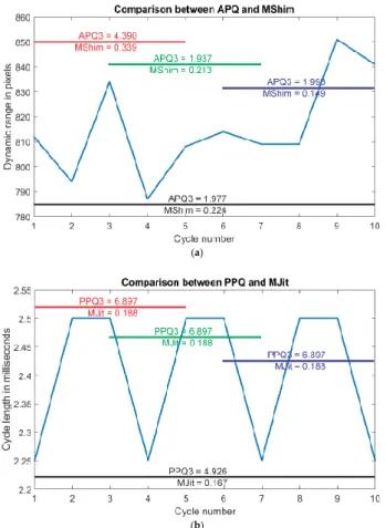
APQ3 only deviated statistically significantly between a sequence length of five analyzed cycles and the larger sequence lengths (with exception of the 5 cycles/100 cycles pairing). This could be the case since APQ3 seems to be generally less stable than comparable parameters like MShim. In Figure 8a, a series of ten consecutive dynamic ranges is depicted for which the difference in behavior between APQ3 and exemplary MShim is clearly visible. For the different intervals of five cycles and the entire ten cycles, APQ3 and MShim were calculated. MShim behaves consistently across the various intervals and the MShim value for all ten consecutive cycles lies in between the values for the shorter intervals.

In contrast, APQ3 varies more strongly for the different five-cycle intervals and additionally the APQ3 value calculated over all ten cycles is lower than the APQ3 value for most of the shorter intervals.

Figure 8b depicts the period lengths for the same subject. In contrast to the dynamic ranges, they are generally much more regular. Hence for this example, the PPQ3 values that are calculated using the same formula as the APQ3 values, but using period lengths instead of dynamic ranges, do not change at all for different starting positions. Since the cycle lengths were more uniform than the dynamic ranges, PPQ3 did not change statistically significantly but

APQ3 did.

(a)

(b)

Figure 8. (a) Dynamic ranges of ten consecutive cycles (bright blue line). Amplitude Perturbation Quotient-3% (APQ3) and Mean Shimmer (MShim) are calculated for different intervals of the total range (red, green, dark blue and black line). (b) Cycle lengths of ten consecutive cycles (bright blue line). Period Perturbation Quotient-3% (PPQ3) and Mean Jitter (MJit) are calculated for different intervals of the total range (red, green, dark blue and black line).

The mean and maximum values and standard deviations for most parameters displayed consistent tendencies and changed most clearly between the shorter sequence lengths (for details see Table 2 and Figures 5–7). Minimum values usually increased with an increasing sequence length without reaching a stable region. The instability of the minimum values for all parameters could be due to the rising probability of changes in phonation with increasing sequence length. Furthermore, it is noteworthy that all Perturbation Quotients (PPQ, APQ and EPQ) behaved clearly distinctively from the other parameters of their groups but rather similar in comparison to each other. This is because they are calculated using the same formula only for different input data [47]. However,

Figure 8. (a) Dynamic ranges of ten consecutive cycles (bright blue line). Amplitude Perturbation Quotient-3% (APQ3) and Mean Shimmer (MShim) are calculated for different intervals of the total range (red, green, dark blue and black line). (b) Cycle lengths of ten consecutive cycles (bright blue line).

Period Perturbation Quotient-3% (PPQ3) and Mean Jitter (MJit) are calculated for different intervals of the

total range (red, green, dark blue and black line).

Appl. Sci.2018,8, 2666 12 of 17

The mean and maximum values and standard deviations for most parameters displayed consistent tendencies and changed most clearly between the shorter sequence lengths (for details see Table 2 and Figures 5–7). Minimum values usually increased with an increasing sequence length without reaching a stable region. The instability of the minimum values for all parameters could be due to the rising probability of changes in phonation with increasing sequence length. Furthermore, it is noteworthy that all Perturbation Quotients (PPQ, APQ and EPQ) behaved clearly distinctively from the other parameters of their groups but rather similar in comparison to each other. This is because they are calculated using the same formula only for different input data [47]. However, except for AVI, none of these changes were found to be statistically significant for comparisons between sequence lengths of 20 cycles and longer sequences. Furthermore, even though systematic increases and decreases were often visually observed up to a sequence length of 50 or 100 cycles (see Table 2), the largest changes were observed for almost all parameters between shorter sequence lengths. Hence, we suggest avoiding smaller sequence lengths than 20 cycles for calculation of all GAW perturbation measures.

Additionally, we suggest avoiding the use of the parameter AVI in general. We make this general suggestion because taking into account the observed often systematic behavior of the descriptive values, it is possible that other more subtle effects exist that were not significant in our analysis. To be able to make a more precise statement, it is necessary to confirm these findings for larger datasets and especially for subjects with vocal disorders.

5. Shortcomings

Since only recordings of healthy females were investigated, the conclusions of this work are not necessarily transferable to male subjects and subjects with voice disorders. Especially for heavily disturbed vocal fold oscillations, the selection of a sequence length greater than 20 cycles for analysis may be necessary.

Since there is a significant overlap of the cycle sets (see Figure 3), the parameters for different sequence lengths are more likely to attain similar values. This overlap was preferred, since otherwise the influences by camera movement and other long-term effects might increase. Additionally this study only provides a small sample size, which limits its statistical significance.

More perturbation parameters than in this evaluated set of parameters may exist. It is also possible that in other works parameters with the same name as the parameters examined in this work are defined differently. In particular, it should be noted that different software tools may deviate significantly in the calculation of various parameters [37,48]. This may limit the transferability of the results of this study to those. Furthermore, other GAW definitions exist that were not considered here [28–31].

6. Conclusions

The comparability of studies using different sequence lengths for GAW perturbation parameter calculations is given with certain limitations. First, the chosen sequence length should be at least 20 cycles to minimize the influence of statistically significant effects on certain parameters. More subtle influences on descriptive values of the investigated parameters were also observed, most clearly between shorter sequence lengths. This further justifies the lower limit of 20 cycles. Second, the parameter AVI is generally not comparable for different GAW sequence lengths. With this study another potential influence factor on voice disorder parameters was investigated, as different other influencing factors on other parameter types were investigated before. This will pave the way to the reduction of the great number of measures in use to a smaller set of meaningful, standardized parameters to greatly improve the information exchange between different studies and the relevance of clinical data.

Supplementary Materials: The following are available online at

s1, Table S1:

p-values of all relevant statistical tests performed.

Appl. Sci.2018,8, 2666 13 of 17

Author Contributions: Conceptualization, M.D. and P.S.; Data Curation, P.S. and A.S.; Formal Analysis, P.S.;

Funding acquisition, M.D. and C.B.; Investigation, P.S. and A.S.; Project Administration, M.D. and A.S.; Resources, M.D. and C.B.; Software, P.S.; Supervision, M.D. and A.S.; Validation, M.S. and M.K.; Writing-original draft, P.S.

and A.S.; Writing-review & editing, M.S., A.S., M.D., P.S. and M.K.

Funding: This research was funded by the Deutsche Forschungsgemeinschaft (DFG) under grants BO4399/2-1 and DO1247/8-1 (number 323308998).

Acknowledgments: We acknowledge the contributions of Pablo Gómez, who helped improving the readability and understandability of this article.

Conflicts of Interest: The authors declare no conflict of interest. The funders had no role in the design of the study; in the collection, analyses, or interpretation of data; in the writing of the manuscript, and in the decision to publish the results.

Appendix A

The Tables A1–A3 list descriptive values for all parameters for period perturbation measures (Table A1), amplitude perturbation measures (Table A2) and energy perturbation measures (Table A3).

Table A1. Group values of all parameters for Period Perturbation Measures (PPM).

Parameter Name and

Sequence Length Average Standard Deviation Maximum Minimum Period Perturbation Measures (PPM)

MJit

0.116 0.079 0.250 0.000

MJit

0.119 0.073 0.222 0.000

MJit

0.120 0.067 0.237 0.026

MJit

0.123 0.059 0.230 0.041

MJit

0.123 0.058 0.222 0.051

Jit(%)

3.742 2.773 10.417 0.000

Jit(%)

3.867 2.610 9.357 0.000

Jit(%)

3.904 2.412 8.399 0.704

Jit(%)

3.941 2.190 9.472 0.960

Jit(%)

3.944 2.221 9.376 1.190

JitFac

3.767 2.828 10.638 0.000

JitFac

3.872 2.606 9.357 0.000

JitFac

3.896 2.389 8.267 0.749

JitFac

3.933 2.160 9.432 0.963

JitFac

3.931 2.176 9.337 1.205

JitRat

37.421 27.730 104.167 0.000

JitRat

38.669 26.103 93.567 0.000

JitRat

39.041 24.125 83.987 7.041

JitRat

39.405 21.900 94.721 9.604

JitRat

39.438 22.205 93.765 11.898

PPQ3

3.566 2.893 10.468 0.000

PPQ3

2.845 2.038 7.037 0.000

PPQ3

2.718 1.758 6.034 0.535

PPQ3

2.647 1.515 6.435 0.668

PPQ3

2.649 1.501 6.307 0.812

PPF

3.764 2.787 10.556 0.000

PPF

3.881 2.608 9.383 0.000

PPF

3.910 2.408 8.363 0.727

PPF

3.942 2.180 9.478 0.962

PPF

3.943 2.204 9.383 1.197

RAP

0.014 0.012 0.042 0.000

RAP

0.020 0.014 0.049 0.000

RAP

0.023 0.015 0.051 0.004

RAP

0.025 0.014 0.060 0.006

RAP

0.026 0.015 0.061 0.008

Appl. Sci.2018,8, 2666 14 of 17

Table A1. Cont.

Parameter Name and

Sequence Length Average Standard Deviation Maximum Minimum Period Perturbation Measures (PPM)

RAP

0.024 0.019 0.069 0.000

RAP

0.025 0.018 0.061 0.000

RAP

0.026 0.017 0.057 0.005

RAP

0.026 0.015 0.063 0.007

RAP

0.026 0.015 0.062 0.008

PVI

1.193 0.782 2.604 0.000

PVI

1.180 0.789 2.770 0.000

PVI

1.175 0.726 2.771 0.213

PVI

1.181 0.613 2.777 0.277

PVI

1.185 0.628 2.777 0.345

Table A2. Group values of all parameters for Amplitude Perturbation Measures (APM).

Parameter Name and

Sequence Length Average Standard Deviation Maximum Minimum Amplitude Perturbation Measures (APM)

MShim

0.151 0.093 0.387 0.047

MShim

0.129 0.060 0.301 0.061

MShim

0.135 0.053 0.272 0.068

MShim

0.134 0.043 0.247 0.064

MShim

0.135 0.038 0.235 0.075

Shim(%)

0.252 0.161 0.656 0.073

Shim(%)

0.214 0.105 0.509 0.096

Shim(%)

0.223 0.092 0.460 0.106

Shim(%)

0.221 0.075 0.416 0.100

Shim(%)

0.223 0.066 0.396 0.116

APQ3

1.558 1.182 4.400 0.310

APQ3

1.006 0.599 2.747 0.334

APQ3

0.916 0.457 2.133 0.356

APQ3

0.883 0.339 1.810 0.397

APQ3

0.877 0.317 1.737 0.425

APF

1.736 1.066 4.470 0.544

APF

1.478 0.696 3.467 0.709

APF

1.553 0.612 3.132 0.790

APF

1.541 0.493 2.833 0.741

APF

1.554 0.443 2.704 0.862

AVI

-0.907 0.366 -0.273 -1.530

AVI

-0.781 0.351 -0.257 -1.470

AVI

-0.493 0.316 0.283 -1.078

AVI

-0.256 0.307 0.231 -0.792

AVI

0.015 0.379 0.910 -0.630

Table A3. Group values of all parameters for Energy Perturbation Measures (EPM).

Parameter Name and

Sequence Length Average Standard Deviation Maximum Minimum Energy Perturbation Measures (EPM)

EPQ3_C5 9.880 7.443 23.847 0.499

EPQ3_C10 7.768 5.175 16.266 0.443

EPQ3_C20 7.395 4.466 14.732 1.777

EPQ3_C50 7.292 3.854 14.781 2.117

EPQ3_C100 7.295 3.701 14.341 2.528

EPF_C5 11.089 6.934 24.424 0.869

EPF_C10 11.108 6.517 21.952 1.209

EPF_C20 11.233 6.209 20.983 2.812

EPF_C50 11.384 5.526 22.090 3.340

EPF_C100 11.392 5.381 21.629 4.210

Appl. Sci.2018,8, 2666 15 of 17

References

1. Titze, I.R. Principles of Voice Production, 2nd ed.; National Center for Voice and Speech: Iowa City, IA, USA, 2000; pp. 87–183.

2. Stevens, K.N. Source Mechanisms. In Acoustic Phonetics; Keyser, S.J., Ed.; MIT Press: Cambridge, MA, USA, 2000; pp. 55–126.

3. Baken, R.J.; Orlikoff, R.F. Vocal fundamental frequency. In Clinical Measurement of Speech & Voice, 2nd ed.;

Cengage Learning: Clifton Park, NY, USA, 1999.

4. Kendall, K.A. Clinical Applications for High-Speed Laryngeal Imaging. In Laryngeal Evaluation; Kendall, K., Leonard, R., Eds.; Georg Thieme: New York City, NY, USA, 2010; p. 272.

5. Švec, J.G.; Schutte, H.K. Videokymography: High-speed line scanning of vocal fold vibration. J. Voice 1996, 10, 201–205. [CrossRef]

6. Echternach, M.; Döllinger, M.; Sundberg, J.; Traser, L.; Richter, B. Vocal fold vibrations at high soprano fundamental frequencies. J. Acoust. Soc. Am. 2013, 133, 82–87. [CrossRef] [PubMed]

7. Deliyski, D. Laryngeal High-Speed Videoendoscopy. In Laryngeal Evaluation; Kendall, K., Leonard, R., Eds.;

Georg Thieme: New York City, NY, USA, 2010; pp. 245–270.

8. Phadke, K.V.; Vydrová, J.; Domagalská, R.; Švec, J.G. Evaluation of clinical value of videokymography for diagnosis and treatment of voice disorders. Eur. Arch. Otorhinolaryngol. 2017, 274, 3941–3949. [CrossRef]

[PubMed]

9. Švec, J.G.; Sundberg, J.; Hertegård, S. Three registers in an untrained female singer analyzed by videokymography, strobolaryngoscopy and sound spectrography. J. Acoust. Soc. Am. 2008, 123. [CrossRef]

[PubMed]

10. Dejonckere, P.H.; Lebacq, J.; Bocchi, L.; Orlandi, S.; Manfredi, C. High-speed single line scan: An application in singing pedagogy. Ephonoscope 2016, 2, 273–286.

11. Deliyski, D.; Hillman, R. State of the art laryngeal imaging: Research and clinical implications. Curr. Opin.

Otolaryngol. Head Neck Surg. 2010, 18, 147–152. [CrossRef] [PubMed]

12. Patel, R.R.; Dubrovskiy, D.; Döllinger, M. Measurement of glottal cycle characteristics between children and adults: Physiological variations. J. Voice 2014, 28, 476–486. [CrossRef] [PubMed]

13. Poburka, B.J.; Patel, R.R.; Bless, D.M. Voice-vibratory assessment with laryngeal imaging (VALI) form:

Reliability of rating stroboscopy and high-speed videoendoscopy. J. Voice 2017, 31, 513.e1–513.e14. [CrossRef]

[PubMed]

14. Zacharias, S.R.C.; Myer, C.M.; Meinzen-Derr, J.; Kelchner, L.; Deliyski, D.D.; Alarcón, A. Comparison of videostroboscopy and high-speed videoendoscopy in evaluation of supraglottic phonation. Ann. Otol.

Rhinol. Laryngol. 2016, 125, 829–837. [CrossRef] [PubMed]

15. Döllinger, M.; Lohscheller, J.; McWhorter, A.; Kunduk, M. Variability of normal vocal fold dynamics for different vocal loading in one healthy subject investigated by phonovibrograms. J. Voice 2009, 23, 175–181.

[CrossRef] [PubMed]

16. Semmler, M.; Kniesburges, S.; Parchent, J.; Jakubaß, B.; Zimmermann, M.; Bohr, C.; Schützenberger, A.;

Döllinger, M. Endoscopic laser-based 3D imaging for functional voice diagnostics. Appl. Sci. 2017, 7.

[CrossRef]

17. Deliyski, D.D.; Petrushev, P.P.; Bonilha, H.S.; Gerlach, T.T.; Martin-Harris, B.; Hillman, R.E. Clinical implementation of laryngeal high-speed videoendoscopy: Challenges and evolution. Folia Phoniatrica et Logopaedica 2007, 60, 33–44. [CrossRef] [PubMed]

18. Mehta, D.D.; Zañartu, M.; Quatieri, T.F.; Deliyski, D.D.; Hillman, R.E. Investigating acoustic correlates of human vocal fold vibratory phase asymmetry through modeling and laryngeal high-speed videoendoscopy.

J. Acoust. Soc. Am. 2011, 130. [CrossRef] [PubMed]

19. Ishikawa, C.C.; Pinheiro, T.G.; Hachiya, A.; Montagnoli, A.N.; Tsuji, D.H. Impact of cricothyroid muscle contraction on vocal fold vibration: Experimental study with high-speed videoendoscopy. J. Voice 2017, 31, 300–306. [CrossRef] [PubMed]

20. Stellan, H. What have we learned about laryngeal physiology from high-speed digital videoendoscopy?

Curr. Opin. Otolaryngol. Head Neck Surg. 2005, 13, 152–156. [CrossRef]

Appl. Sci.2018,8, 2666 16 of 17

21. Rasp, O.; Lohscheller, J.; Döllinger, M.; Eysholdt, U.; Hoppe, U. The pitch rise paradigm: A new task for real-time endoscopy of non-stationary phonation. Folia Phoniatrica et Logopaedica 2006, 58, 175–185. [CrossRef]

[PubMed]

22. Zacharias, S.R.C.; Deliyski, D.D.; Gerlach, T.T. Utility of laryngeal high-speed videoendoscopy in clinical voice assessment. J. Voice 2018, 32, 216–220. [CrossRef] [PubMed]

23. Patel, R.; Dailey, S.; Bless, D. Comparison of high-speed digital imaging with stroboscopy for laryngeal imaging of glottal disorders. Ann. Otol. Rhinol. Laryngol. 2008, 117, 413–424. [CrossRef] [PubMed]

24. Hartnick, C.J.; Zeitels, S.M. Pediatric video laryngo-stroboscopy. Int. J. Pediatr. Otorhinolaryngol. 2005, 69, 215–219. [CrossRef] [PubMed]

25. Vaca, M.; Cobeta, I.; Mora, E.; Reyes, P. Clinical assessment of glottal insufficiency in age-related dysphonia.

J. Voice 2017, 31, 128.e1–128.e5. [CrossRef] [PubMed]

26. Stemple, J.C.; Fry, L.B. Performing Videostroboscopy. In Laryngeal Evaluation; Kendall, K., Leonard, R., Eds.;

Georg Thieme: New York City, NY, USA, 2010; p. 110.

27. Wendler, J.; Seidner, W.; Eysholdt, U. Lehrbuch der Phoniatrie und Pädaudiologie, 4th ed.; Thieme: Stuttgart, Germany, 2005; pp. 113–120.

28. Noordzij, P.J.; Woo, P. Glottal Area Waveform Analysis of Benign Vocal Fold Lesions before and after Surgery.

Ann. Otol. Rhinol. Laryngol. 2000, 109, 441–446. [CrossRef] [PubMed]

29. Mendez, A.; Gracia, B.; Ruiz, I.; Iturricha, I. Glottal Area Segmentation without Initialization using Gabor Filters. In Proceedings of the IEEE International Symposium on Signal Processing and Information Technology (ISSPIT), Sarajevo, Bosnia and Herzegovina, 16–19 December 2008. [CrossRef]

30. Kunduk, M.; Yan, Y.; McWhorther, A.J.; Bless, D. Investigation of voice initiation and voice offset characteristics with high-speed digital imaging. Logop. Phoniatr. Vocol. 2006, 31, 139–144. [CrossRef]

[PubMed]

31. Chen, X.; Bless, D.; Yan, Y. A Segmentation Scheme Based on Rayleigh Distribution Model for Extracting Glottal Waveform from High-speed Laryngeal Images. In Proceedings of the 27th Annual International Conference of the Engineering in Medicine and Biology Society (IEEE-EMBS), Shanghai, China, 17–18 January 2006. [CrossRef]

32. Patel, R.R.; Unnikrishnan, H.; Donohue, K.D. Effects of vocal fold nodules on glottal cycle measurements derived from high-speed videoendoscopy in children. PLoS ONE 2016, 11. [CrossRef] [PubMed]

33. Petermann, S.; Döllinger, M.; Kniesburges, S.; Ziethe, A. Analysis method for the neurological and physiological processes underlying the pitch-shift reflex. Acta Acust. United Acust. 2016, 102, 284–297.

[CrossRef]

34. Deliyski, D.D.; Shaw, H.S.; Evans, M.K. Influence of sampling rate on accuracy and reliability of acoustic voice analysis. Logop. Phoniatr. Vocol. 2005, 30, 55–62. [CrossRef] [PubMed]

35. Schützenberger, A.; Kunduk, M.; Döllinger, M.; Alexiou, C.; Dubrovskiy, D.; Semmler, M.; Seger, A.; Bohr, C.

Laryngeal high-speed videoendoscopy: Sensitivity of objective parameters towards recording frame rate.

BioMed Res. Int. 2016, 2016. [CrossRef] [PubMed]

36. Scherer, R.; Vail, V.; Guo, C. Required number of tokens to establish reliable voice perturbation values.

NCVS Status Prog. Rep. 1994, 7, 107–117.

37. Karnell, M.P.; Hall, K.D.; Landahl, K.L. Comparison of fundamental frequency and perturbation measurements among three analysis systems. J. Voice 1995, 9, 383–393. [CrossRef]

38. Hohm, J.; Döllinger, M.; Bohr, C.; Kniesburges, S.; Ziethe, A. Influence of F_0 and sequence length of audio and electroglottographic signals on perturbation measures for voice assessment. J. Voice 2015, 29, 517.e11–517.e21. [CrossRef] [PubMed]

39. Bohr, C.; Kraeck, A.; Eysholdt, U.; Ziethe, A.; Döllinger, M. Quantitative analysis of organic vocal fold pathologies in females by high-speed endoscopy. Laryngoscope 2013, 123, 1686–1693. [CrossRef] [PubMed]

40. Patel, R.R.; Walker, R.; Sivasankar, P.M. Spatiotemporal quantification of vocal fold vibration after exposure to superficial laryngeal dehydration: A preliminary study. J. Voice 2016, 30, 427–433. [CrossRef] [PubMed]

41. Vlot, C.; Ogawa, M.; Hosokawa, K.; Iwahashi, T.; Kato, C.; Inohara, H. Investigation of the immediate effects of humming on vocal fold vibration irregularity using electroglottography and high-speed laryngoscopy in patients with organic voice disorders. J. Voice 2017, 31, 48–56. [CrossRef] [PubMed]

42. Arbeiter, M.; Petermann, S.; Hoppe, U.; Bohr, C.; Döllinger, M.; Ziethe, A. Analysis of the auditory feedback

and phonation in normal voices. Ann. Otol. Rhinol. Laryngol. 2017, 127, 89–98. [CrossRef] [PubMed]

Appl. Sci.2018,8, 2666 17 of 17

43. Krausert, C.R.; Liang, Y.; Zhang, Y.; Rieves, A.L.; Geurink, K.R.; Jiang, J.J. Spatiotemporal analysis of normal and pathological human vocal fold vibrations. Am. J. Otolaryngol. 2012, 33, 641–649. [CrossRef] [PubMed]

44. Horii, Y. Vocal shimmer in sustained phonation. J. Speech Lang. Hear. Res. 1980, 23, 202–209. [CrossRef]

45. Hollien, H.; Michel, J.; Doherty, T.E. A method for analyzing vocal jitter in sustained phonation. J. Phon.

1973, 1, 85–91.

46. Horii, Y. Fundamental frequency perturbation observed in sustained phonation. J. Speech Lang. Hear. Res.

1979, 22, 5–19. [CrossRef]

47. Kasuya, H.; Endo, Y.; Saliu, S. Novel acoustic measurements of jitter and shimmer characteristics from pathological voice. In Proceedings of the EUROSPEECH’93, Berlin, Germany, 22–25 September 1993;

pp. 1973–1976.

48. Bielamowicz, S.; Kreiman, J.; Gerratt, B.; Dauer, M.; Berke, G. Comparison of voice analysis systems for perturbation measurement. J. Speech Hear. Res. 1996, 39, 126–134. [CrossRef] [PubMed]

49. Koike, Y. Application of some acoustic measures for the evaluation of laryngeal dysfunction. Stud. Phonol.

1973, 7, 17–23. [CrossRef]

50. Deal, R.E.; Emanuel, F.W. Some waveform and spectral features of vowel roughness. J. Speech Lang. Hear. Res.

1978, 21, 250–264. [CrossRef]

51. Schlegel, P.; Stingl, M.; Kunduk, M.; Kniesburges, S.; Bohr, C.; Döllinger, M. Dependencies and ill-designed parameters within high-speed videoendoscopy and acoustic signal analysis. J. Voice 2018. [CrossRef]

[PubMed]

52. Lohscheller, J.; Döllinger, M.; Schuster, M.; Eysholdt, U.; Hoppe, U. The laryngectomee substitute voice:

Image processing of endoscopic recordings by fusion with acoustic signals. Methods Inf. Med. 2003, 42, 277–281. [CrossRef] [PubMed]

© 2018 by the authors. Licensee MDPI, Basel, Switzerland. This article is an open access

article distributed under the terms and conditions of the Creative Commons Attribution

(CC BY) license (http://creativecommons.org/licenses/by/4.0/).