Casimir Forces and Geometry

(1)

Casimir Forces and Geometry

Inaugural-Dissertation zur

Erlangung des Doktorgrades

der Mathematisch-Naturwissenschaftlichen Fakultät der Universität zu Köln

vorgelegt von

Rauno B¨uscher

aus G¨ottingen

2005

(2)

Dr. T. Emig

Tag der m¨undlichen Pr¨ufung: 6. Juli 2005

(3)

1

Abstract

Casimir interactions are interactions induced by quantum vacuum fluctuations and thermal fluctuations of the electromagnetic field. Using a path integral quantization for the gauge field, an effective Gaussian action will be derived which is the starting point to compute Casimir forces between macroscopic objects analytically and numerically. No assumptions about the independence of the material and shape dependent contributions to the interaction are made. We study the limit of flat surfaces in further detail and obtain a concise derivation of Lifshitz’ theory of molecular forces [73]. For the case of ideally conducting boundaries, the Gaussian action will be calculated explicitly. Both limiting cases are also discussed within the framework of a scalar field quantization approach, which is applicable for translation- ally invariant geometries. We develop a non–perturbative approach to calculate the Casimir interaction from the Gaussian action for periodically deformed and ideally conducting objects numerically. The obtained results reveal two different scaling regimes for the Casimir force as a function of the distance between the objects, their deformation wavelength and amplitude. The results confirm that the interaction is non–additive, especially in the presence of strong geometric deformations. Furthermore, the numerical approach is extended to calculate lateral Casimir forces. The results are consistent with the results of the proximity–

force approximation for large deformation wavelengths. A qualitatively diﬀerent behaviour between the normal and lateral force is revealed. We also establish a relation between the boundary induced change of the density of states for the scalar Helmholtz equation and the Casimir interaction using the path integral method. For statically deformed boundaries, this relation can be expressed as a novel trace formula, which is formally similar to the so–called Krein–Friedel–Lloyd formula [64]. While the latter formula describes the density of states in terms of the S–matrix of quantum scattering at potentials, the new trace formula is applied to the free Green function, evaluated at the boundary surfaces of the conﬁning geometry.

This latter formulation is non–approximative and hence exact.

(4)

(5)

3

A Introduction

1 Fluctuation induced interactions

Casimir interactions are one of the manifestations of quantum physics which can not be explained classically. The classical notion of vacuum is an empty space where all particles are removed. Imagine this classical vacuum being free of ﬁelds, so that quantum mechanical particles as photons are also removed. The problem now is that classical voidness has no quantum mechanical analogon. Heisenbergs uncertainty principle sets the limit of knowledge of pairs of physical parameters as the positionxand the momentumpof a particle to the order of Planck’s constant, ∆x·∆p≥ /2. Another pairing is time and energy, ∆E·∆t≥ /2, which forbids the precise knowledge of an unique value for the energy of a system at a unique point in time. The quantum mechanical solution is to assume the existence ofﬂuctuations.

Particles are smeared out by considering them as probability distributions with a finite width around an average value (which corresponds to the classical point–like value), they can merge ”virtually” within a given time interval and carry an energy which is allowed by the time–energy uncertainty relation. Quantum mechanics allows for the existence of zero–point energy, and a foam of virtual particles and fields in the ”vacuum”. Since the geometry of spacetime and the existence of particles and fields are linked with each other, the fluctuations on Planck scale also concern the topology of spacetime itself, see Fig. A.1.

Naturally, the question arises if these quantum fluctuations can have an influence on the interaction of microscopic or even macroscopic objects. This is in fact the case. To begin with, the notion of fluctuation induced interactions shall be clarified from a more general point of view. Obviously, fluctuations exist at small length scales, but not merely there.

They can also be of classical or thermal nature. To capture an idea of interactions caused by fluctuations, a fluctuating medium is to be considered, as e.g. the zero point fluctuations of the electromagnetic field, and secondly, objects which are immersed into that medium. In case of the electromagnetic field, one can think of atoms, dipole molecules or more macroscopic objects like conductors. If the mere presence of the objects modifies the fluctuations, these objects will get into interactionvia the change of the fluctuations of the medium. For example, the surface of a conductor poses the constraint that the tangential components

(8)

Figure A.1: Fluctuating space–time.

(see www.casimir.rl.ac.uk)

Figure A.2: Fluctuation induced pressure.

of the electric field vanish on it. This suppresses some fluctuations of the zero point field compared to the spacewithout the conductor. This change of fluctuations determines the interaction between the conductor surfaces. An example for thermal fluctuations is given by the Brownian motion of a particle. The locations of the particle are characterized by a Boltzmann distributione⁻Û⁽^r⁾^/k^B^T with the potentialU(r)at each positions. Fluctuations in the movement are then of the order∼k_BT. The van–der–Waals force provides an example for classical fluctuation induced forces.

Fluctuation induced interactions between objects depend on the characteristic features of the objects as their topology or material properties. These features take influence on the boundary constraints which are imposed on the fluctuating field. On the other hand, the kind of field on which these conditions are imposed govern the interaction between the objects.

Fluctuation induced interactions have a broad range of relevance, cf. Refs. [83, 78, 14, 91].

To give some examples, they are important e.g. in cosmology since they are related to zero point energies of fields [111]. Fluctuations of gluon fields confined by boundaries were discussed in [81, 82], see also [21]. But they are also important in exotic areas such as the physics related to biological problems including the dynamic behaviour of membranes [92, 93, 47, 85, 86], or the sticking of large molecules as proteins on membranes which is

(9)

A1 Fluctuation induced interactions 7

related to the theory of correlated ﬂuids [60].

The Casimir force is a striking example that vacuum fluctuations are not merely a theoretical construct but have real consequences. This makes the Casimir effect globally significant not only to quantum physics, but in all fields where fluctuation induced phenomena occur, cf. [56, 78, 83, 60].

Figure A.3: Hendrik Brugt Ger- hard Casimir (1909 – 2000).

We return to the quantum fluctuations of the electromagnetic field. While quantum fluctuations can be expected for any quantum field, especially for the electromagnetic field, which is a long ranged fundamental interaction, mea- surable effects can be expected. The zero point energy of the vacuum state is formally infinite and it is commonly disregarded by normal ordering the Hamiltonian, since it is a constant which commutes with the creation and an- nihilation operators of photons and has therefore no influence on the quantum dynamics governed by the Heisen- berg equations of motion. However, the vacuum energy is not arbitrary and subject to changes due to boundary constraints. In fact, these are observable, as predicted by Hendrik Casimir in the year 1948 [22]. Between two infinitely extended parallel conducting plates at distance H, Casimir predicted anattractiveforce per surface area Aof

F₀

A =−π² 240

c

H⁴ (A1.1)

at zero temperature.

The presence of the plates constricts the quantized normal photon modes in the cavity between the plates. They are described by harmonic oscillators with wave vector k = (kx, ky, πn/H) and frequency ω(k) =c|k|, and their ground state energy is ω(k)/2. The ground state energy of the vacuum in the presence of the two plates is given by the sum over all modes of these energy contributions, /2

kω(k). This zero point energy is formally infinite and must be regularized, which can be done by subtracting the asymptotic expression of the sum for infinite surface distance. The force F₀ is given by the derivative of the regularized energy with respect to the plate distance. A detailed calculation is given e.g. in Ref. [78]. The boundary induced restrictions to the field fluctuations inside the gap between the surfaces and outside beyond the gap leads to a difference of radiation pressures of the fluctuating zero point field, which induces theattractiveCasimir force between the surfaces.

(10)

This is illustrated in Fig. A.2. Historically, Casimir’s work was rooted in studies of colloidal suspensions. The stability of those suspensions was explained by the interplay of repulsive and attractive forces, where the attractive force was attributed to the London van–der–Waals interaction at short distances. Experiments showed that for large colloidal molecules [110], retardation due to the ﬁnite velocity of light has to be taken into account for the interaction.

Casimir and Polder [23] demonstrated that the London van–der–Waals inter atomic potential U(r)∼ −r⁻⁶ is modiﬁed by retardation and falls of as U(r) ∼ −α₁α₂ c/r⁷, where α₁, α₂ are the static polarizabilities of the interacting molecules. For a deeper understanding of this result and inspired by an advice from Bohr, who noted that the van–der–Waals force ”must have something to do with zero point energy”, Casimir found that the retarded van–der–

Waals interaction between ﬂuctuating dipoles can be related to the change of the zero point energy of the electromagnetic ﬁeld generated by the presence of the dipoles. This thread gave the motivation to consider metallic plates.

Ë

¾

Ë

½

Figure A.4: Proximity force approximation (PFA). The curved boundary surfaces are approx- imated locally by ﬂat surface segments.

The ﬁrst experiments to detect Casimir interactions macroscopically were performed by Abricosova and Derjaguin in 1951 with dielectric materials [28, 29], namely with a ﬂat glass plate and spherical lenses with radii of R = 10 cm and R = 25 cm. The distance between the plate and the lenses were taken between H = 0.07µm and H = 0.5µm.

This configuration is easier to adjust than the exact par- allelization of two flat plates. The finite curvature of the lens can be well accounted for by the ”Derjarguin approximation” [27] or proximity force approximation (PFA). The PFA method considers the sum of local contributions to the interaction from small flat surface elements opposite to each other, assuming that they behave as infinitesimally small parallel plates. This phenomenological approach is restricted to surfaces that have a small degree of non- parallelism. This is a small local curvature in the case of curved surfaces, as in Derjaguin’s experiments for a plate and a sphere, where the radius of the sphere is much larger than the minimum distance between the surfaces. How- ever, if the curvature becomes larger, the distance between the small flat surface elements changes rapidly, it can no longer be determined unambiguously, see Fig. A.4, and the assumption of summing local contribution becomes unreliable due to diffraction effects.

(11)

Experiments with flat glass plates with distances betweenH= 0.6µm andH= 1.5µm were performed by Overbeek and Sparnaay (1954) [95]. The first experiment with conducting aluminium plates to verify Eq. (A1.1) was performed by Sparnaay (1958) [102] at distances between H= 0.5µm andH = 2µm. The results agreed qualitatively with Casimir’s prediction, at best. Further early experiments are reviewed in [55]. Their problems were mainly technical, e.g. the alignment of the plates or the avoidance of residual charges. But later high precision experiments [68, 87] confirm Casimir’s theoretical prediction to high accuracy.

These experiments will be discussed in the following section in more detail.

Î

½

Ü

¼ Î

¾ Ý

Ü

Figure A.5:Pair–wise summation of potentials (PWS) to calculate van–der–Waals forces between macroscopic bodies of arbitrary shape. The interaction between two dipoles xandy is not independent from the presence of other dipoles, asx. The assumption of perfect conductivity of the surfaces

which led to Eq. (A1.1), is idealized. These surfaces are reflecting for the electromagnetic spectrum at all wavelengths. However, since any real metal becomes trans- parent for frequencies larger than the plasma frequency of the material, a frequency cutoff is effectively posed by real surfaces. Since the main contribution to the force results from modes with wavelengths of the order of the surface distance, Eq. (A1.1) is expected to hold if the distance H between the surfaces is large compared to the plasma wavelength λp, which is of the order of 0.1 to 10 microns in recent experiments. For smaller H, the force will be reduced compared to the ideal result F₀ in Eq. (A1.1).

On the theoretical side, a way to include finitely conducting boundaries is to consider the van–der–Waals interaction of fluctuating dipoles in the materials and to sum over the pair–wise contributions of the dipole interaction. This approximative method is known as pair–wise summation of potentials (PWS). However, it was early recognized that the van–der–Waals interaction is in general not additive, i.e. the interaction between two atoms is influenced by the presence of a third atom, see Fig. A.5. The additivity assumption is justified for dilute media only, where the distances between the interacting molecules are large. The

alteration of the interaction due to the additivity assumption is illustrated by a model calculation in Ref. [78], which shows that the pair–wise summation of Casimir–Polder potentials between a single molecule and an inﬁnite conducting half space leads to a force which is about 80%of the real Casimir force between them.

(12)

The discrepancies between the results from the early experiments with dielectric materials and the theoretical results based on this microscopic assumption of pair wise additivity of intermolecular Casimir–Polder potentials for the van–der–Waals interaction gave the stim- ulus to search for a theoretical description which allows for ﬁnite conductivity beyond the microscopic additivity assumption.

This was achieved by Lifshitz in 1956, who developed amacroscopictheory of the ﬂuctuation induced forces between dielectrics [73], see also [69], by treating the dielectric matter as continua with a frequency dependent dielectric susceptibility (ω). In the limit of ideal conductivity, Lifshitz’ result reduces to Casimir’s result, cf. Eq. (A1.1). In the opposite limit of dielectric susceptibilities close to unity, the result is in coincidence with the microscopic approach of pair–wise summation of retarded van–der–Waals potentials [31, 32]. Lifshitz solved Maxwell’s equations in two half spaces ﬁlled with dielectric media and in the vacuum gap in between with the standard matching conditions at the boundary surfaces. In general, any dielectric medium can be assumed instead of the vacuum gap. The equations read

∇ ×E = iω

c B, (A1.2)

∇ ×B = −iω

c (ω)E−iω

c K. (A1.3)

Here, a random source fieldKis introduced to account for the quantum fluctuations of the field. The fluctuation–dissipation relation enforces the correlations

K_i(x)K_j(x)

= 2 Im(ω)δ_ijδ⁽³⁾

x−x

, (A1.4)

so that only the dissipative part of the dielectric function described by Im(ω) matters.

From this relation, correlation functions for the fields are calculated, and from the latter, the Maxwell stress tensor is obtained. The Casimir pressure onto the (flat) surfaces is then calculated from the zz–component of the stress tensor. The Lifshitz theory for the interaction of dielectric media is generally accepted as to the description of Casimir forces between real dielectric media since it had been supported by accurate experiments which measure the thinning of liquid Helium films with an acoustic interferometry technique [96].

Further experiments conﬁrming the Lifshitz theory were performed by Van Blokland and Overbeek 1978 [106] on chromium. Other experiments are reviewed by Derjaguin et. al.

[30] and Sparnaay [103], a more recent review is provided by Elizalde et. al. [33].

In 1968, van Kampen and collaborators [107] rederived the Lifshitz theory in the non–retarded limit. The concept behind their approach was similar to Casimir’s idea of considering the ﬂuctuations of the zero point energy, but with dielectric boundaries instead of ideal metals.

This approach was extended in 1973 to the general case including retardation [70, 99]. But

(13)

in this approach, absorption does not show up explicitly, which is reﬂected by the fact that only a real dielectric function occurs, contrary to the Lifshitz theory which is based on the ﬂuctuation–dissipation–relation and requires for a complex dielectric function. Barash and Ginzburg proved the equivalence of both approaches in 1973 [10].

An alternative approach to the description of Casimir forces without direct reference to the fluctuations of the vacuum field was provided by Schwinger’s source theory in the year 1978 [100, 101], see also [77, 80]. Schwinger considers the radiation reaction or source fields induced between dipoles to derive the Casimir forces. However, the dipole radiation reaction field is linked to the fluctuating zero point field by the fluctuation–dissipation relation. This explains the deducibility of the Casimir force using Schwinger’s more unconventional concept of source fields and thus the equivalence to Casimir’s vacuum field approach, although the physical premises of both approaches appear to be different. In fact, the normal ordering of equal time Heisenberg–picture photon operators avoids an immediate reference to the zero point vacuum field and requires the source field description. This kind of dual description either via source fields or via the vacuum field had also been performed for the Lamb shift [65].

Although the Lifshitz theory was a significant advance in the theoretical description of macroscopic van–der–Waals or Casimir interactions between real matter, its applicability to general geometries is limited. The problem with Lifshitz’ approach is that it is not suited to surfaces with arbitrary deformations, because then, the solution of Maxwell’s equations in different regions with matching conditions at the boundary surfaces becomes unpracticable. This difficulty equally applies to the approach of van Kampen and collaborators, who also considered the problem of half spaces separated by infinitely extended flat planes as boundaries.

However, the Casimir interaction is expected to be strongly dependent on geometry, and, even the sign of the interaction can vary with geometry, as shown by Boyer, who predicted a repulsive Casimir interaction for an ideally conducting sphere [18]. In contrast to that, the local van–der–Waals interaction between two single neutral molecules is always attrac- tive. This distinct microscopic and macroscopic behaviour underlines the non–additivity of ﬂuctuation forces.

The important and natural question is how the successful Lifshitz theory can be generalized to include surface deformations. Corrections due to geometric deformations and material dependent or thermal corrections to the ideal Casimir force in Eq. (A1.1) had been discussed independently so far. This seems to be reasonable for the case that the characteristic length scales of each of the modifications are widely different from each other. However, this assumption is often not justified.

So far, the proximity–approximation method had mostly been used to account for geometries in experiments which are ”similar” to the system of two ﬂat plates, as e. g. the geometry

(14)

consisting of a plate and a sphere where R H. In arbitrary geometries, however, the PFA can no longer be expected to be applicable, since it becomes unreliable for objects with large curvatures. Contrary to that, the PWS is not affected by short scale changes of the surface structure at small distances. To take the non–additivity of the interaction into account, Mostepanenko and Sokolov [89] proposed a normalization of the Casimir–Polder potential such that the pair–wise summation over two half spaces at distanceH yields the exact result for two flat plates. However, correlation effects between surface deformations and the non–additivity are not taken into account by performing this normalization.

On the theoretical side, the changeover to the generalization of the description of the most simple system of two flat plates to systems with deformed surfaces is non–trivial even for ideal metals. It is not merely a technical difficulty, but rather of fundamental nature and closely related to the spectral theory of quantum systems confined by arbitrary geometries [39].

The famous question ”Can one hear the shape of a drum ?” was posed by Kac in 1966 [59], illustrating the problem of deducing the shape of a region from its resonance spectrum. 26 years later, this question was negated [51], however, the inverse problem of characterizing the resonance spectrum for a given geometry is not yet solved in general. Pioneering work in this field had been done by Balian and Bloch [2, 3, 4, 5, 6], and Duplantier [7]. Balian and Bloch studied the scalar field wave equation by means of multiple reflection expansions for a closed cavity [2]. This work was extended to the characterization of electromagnetic eigenmodes in cavities [3] and the study of geometric properties of the eigenmodes [5]. A semi-classical calculation of the Green function of a quantum mechanical system which is related to the resonance spectrum was developed by Gutzwiller [52] by considering only closed orbits in phase space. These concepts of spectral theory are closely related to the Casimir problem. The Casimir interaction is highly sensitive to variations of the geometric boundaries, this sensitivity translates to the spectrum {ω(k)} of eigenfrequencies of the photon modes. The analytic knowledge of the spectrum would imply a solution of the Casimir problem for arbitrary geometries. The multiple scattering approach was later considered for the Casimir interaction by Balian and Duplantier [7, 8], it reduces to ray optics in the limit of high frequencies. Recently, Jaffe and collaborators [58] proposed a new approach to calculate the Casimir interaction between deformed metals based on ray optics considering the contributions of all classical optical paths between the boundary surfaces. Schaden and Spruch [97, 98] applied Gutzwiller’s semi-classical approach to calculate the Casimir interaction in some simple geometries of ideal metals, as plate and sphere.

Thermal corrections to the Casimir force were also accounted for by Lifshitz [73]. Later in 1967, Mehra [76] inferred from a quantum statistical calculation an additional temperature correction which does not appear in Lifshitz’ theory. It was stated that corrections due to

(15)

A2 High precision experiments and applications 13

thermal ﬂuctuations become important for distances beyond 3µm. At T ≈ 300K, where most experiments are performed, the de Broglie wavelength of photons is λ_T = _k ^c

BT ≈ 7µm. It was postulated that temperature increases the force by 15% at a plate distance of 3µm [61]. Since a deviation from Casimir’s prediction of this magnitude was not observed in the measurement of Lamoreaux [68], the inﬂuence of temperature on the Casimir interaction is an object of current debate [84]. Since the dominant contribution to the force results from frequencies ω ∼ H⁻¹, for experiments in the range of H ≈ 1µm, the dominant contributions are from frequencies in the infrared and visible regime, where the Drude model (ω) = 1−ω²_p/ω² is proposed as to describe real metals [66, 67], where ω_p is the plasma frequency of the metal.

The quantum field theoretical treatment of the Casimir effect with path integral quantization was introduced in 1984 by Bordag, Robaschik and Wieczorek [15], later in 1991 independently also by Li and Kardar [71, 72], who considered the interaction of deformed manifolds in a fluid with long ranged correlations. This approach allows to include arbitrarily deformed manifolds on which any kind of boundary condition can be implemented. This feature makes the approach promising for an analysis of arbitrary geometries. Emig et. al. [35, 36]

developed a perturbation theory for the deformation of ideally conducting surfaces based on this method. Finite conductivity can be accounted for by a suitable choice of boundary conditions. The field theoretical approach is also interesting for the dynamic Casimir effect, where the interacting objects are not assumed to be stationary. The dynamic Casimir effect includes moving objects or fluctuating surfaces, as membranes. The creation of radiation by moving mirrors was studied for a one dimensional cavity [88]. This has received attention due to its connections to Hawking and Unruh effects which describe the radiation from black holes and accelerated masses, respectively. A deeper understanding of these connections is expected to be beneficial for QED, relativity and cosmology [111, 26].

2 High precision experiments and applications

While Sparnaay’s Casimir force measurement in 1958 [102] could only assert a qualitative coincidence with Casimir’s result Eq. (A1.1) and the uncertainty was about 100%, in the year 1997 S. K. Lamoreaux measured the Casimir force between a spherical lens of radius R= 11.3±0.1 cm and a flat plate with a diameter of2.54cm at distances between0.6µm and6µm in an evacuated vessel [68]. The lens is fixed at a micro-positioning device controlled by a piezoelectric stack, while the flat plate is mounted onto one arm of a torsion pendulum.

Both the lens and the plate were gold coated. The other arm of the pendulum is connected to the central electrode of a pair of planar capacitors. Applying voltages to the capacitors

(16)

allow for a measurement of the restoring force required to balance the pendulum for any torque caused by the Casimir force between lens and sphere. This way, Casimir’s prediction could be veriﬁed within5% of accuracy.

Roy and Mohideen [87] performed an improved measurement with an atomic force microscope and reached an agreement between experiment and theory of up to1%. They used a similar geometric setup with an aluminium coated polystyrene sphere of a diameter of200±4µm mounted on a cantilever, see Fig. A.7. The distance to the aluminium coated plate was taken in the range of 0.1µm to 0.9µm. Instead of a torsion pendulum, a deviation of the distance between plate and sphere is detected by a laser beam reﬂected at the cantilever, which is registered by a pair of photo diodes. A piezo stack is used to bring the ﬂat plate close to the sphere, see Fig. A.7.

In a similar experimental assembly, Chen, Mohideen and co–workers in 2002 [25] demonstrated the existence oflateralCasimir forces predicted before [35, 36] which act tangentially between deformed surfaces. They used a plate with uniaxial sinusoidal corrugation of period 1.2µm and a sphere of the same diameter of200±4µm with gold coating, on which another sinusoidal corrugation with diﬀerent amplitude was imprinted. The amplitudes of corrugation on the sphere and the plate were measured with the atomic force microscope as59±7 nm and8±1 nm, respectively. The lateral force was measured for a mean distance (which is understood to be the minimum distance between plate and sphere without the corrugation) in the range between 0.2µm and 0.3µm. The measured force exhibits the periodicity corresponding to the corrugations.

Figure A.6: Experimental setup of Lamoreaux.

Picture from Scientiﬁc American & S. K. Lam-

oreaux. Figure A.7: Mohideen’s experiment [87].

(17)

A2 High precision experiments and applications 15

A few months prior to this experiment, Chan et. al. at the Bell Laboratories of Lucent Tech- nologies recognized the influence of the Casimir force on Micro– and Nano–electromechanical systems (MEMS,NEMS) due to their topological nature associated with the dependence on the boundary of the electromagnetic field [38]. Boyer’s result [18] suggests that the Casimir interaction can strongly be influenced in artificial microstructures. A generally more unde- sired effect in MEMS which has been ascribed to theattractiveCasimir force is the sticking of mobile components [19]. Chan’s group realized experimentally a driven micromechanical anharmonic oscillator the anharmonic behaviour of which is induced by the Casimir force and thus showed the influence of the Casimir interaction even on dynamic features of MEMS [24].

Chan and Garcia also studied experimentally the critical Casimir force caused by thermal order parameter fluctuations in Helium films near the critical point. They performed an experiment which shows the thinning of⁴He–films absorbed on a stack of copper electrodes near the super fluid transition [43], see also Refs. [44, 105, 54].

Figure A.8: Micromecanical Os- cillator [24].

The latter experiments make explicit that a potential area of application of Casimir interactions lay in micro– and nanotechnological applications as MEMS and NEMS. Pri- marily, it would be interesting if surface geometries can be designed in a way to avoid the sticking of mobile parts. Re- lated to this is the question if repulsive forces can appear between disconnected surface components [74]. There is still an amount of theoretical work to be done to answer this question. It can be expected that a combination of normal and lateral Casimir forces by a suitable design of surface proﬁles can be used to construct ratchet–like machines which can rectify ﬂuctuations using the Casimir force.

(18)

B Casimir interaction between dielectric materials

The aim of this chapter is to develop an approach for the calculation of molecular interactions between macroscopic surfaces of general shape. The approach is based on the path integral quantization of the fluctuating electromagnetic fieldA^µ. In the free vacuum space, the field quantization is described by the vacuum partition function

Z =

[A]e^iS^{^A^}, (B0.1)

which is governed by the Gaussian actionS{A}. Here and in the following, we choose unities such that= 1and c= 1.

The path integral quantization had been applied to calculate fluctuation induced interactions for ideal metals at zero temperature, cf. Refs. [15, 13, 16, 48, 60, 35, 72]. Whereas ideal metals can be described by local boundary conditions for the field components, this is no longer possible for real materials. We will use non–local boundary conditions to describe the interaction of the fluctuating field with the material boundaries. The viewpoint of describing the interaction by field fluctuations in the vacuum with boundary conditions differs from the more elaborated approach of considering the field fluctuations outside andinside of the materials [73, 31, 32].

These non–local boundary conditions for the gauge field A^µ are based on the extinction theorem of classical electrodynamics, see Refs. [41, 94, 17]. The guiding idea behind this theorem is that an incident field (in the vacuum) induces dipole flutuations in the material. The field of the dipole fluctuations propagates inside the material and a part of it extinguishesthe incoming field. For this reason the theorem is called ”extinction”–theorem.

Macroscopically, this extinction can be viewed as causedat the surfaceof the material, see e.g. Ref. [78]. Thus, the theorem establishes a relation between field fluctuations outside and inside of a material via boundary conditions for the quantized field modes, which can be viewed as non–penetrable.

The boundary conditions allow to consider material properties, described by the frequency dependent dielectric function (ω), and geometric deformations simultaneously, i.e. no as-

(19)

B1 General approach for material boundaries 17

sumptions are made about the correlations between contributions to the force from geometry and material.

An effective Gaussian action is obtained from a path integral quantization. This action is a functional of the dielectric function and the profile function which determines the geometry of the surface, and it serves as a basis for further analytical (e.g. perturbative) or numerical computations to study correlations between material properties and geometry. Thermal fluctuations at finite temperatures are included straightforwardly within this description.

The formalism will be tested by studying first the limit of flat surfaces. This yields the results found by Lifshitz [73] for the interaction of two flat surfaces of real materials in a concise way and without the need to solve Maxwell’s equations in separated regions and to considering stress tensor calculations, as done originally by Lifshitz. The Lifshitz theory can also be derived within a scalar field approach. Although this works strictly only for flat surfaces, it is very compact and can be compared with other approaches [107, 70]. Secondly, we consider the action in the limit of ideal metals, where it can be calculated explicitly. A perturbative analysis for this action had been performed in [35, 36] as well as in [34]. An analytic and numeric analysis of this limit will be performed for periodic geometries in later chapters.

1 General approach for material boundaries

We will develop a macroscopic theory which allows to calculate the interaction between materials of rather general shape. Instead of considering directly the field emitted by the fluctuating dipoles in the material, we consider the interaction as generated by the modifications of the quantum (and thermal) fluctuations of the electromagnetic field between the materials. No direct reference is made to the electromagnetic field fluctuations in the interior of the materials. The effect of the dipoles induced by the external fluctuating field will be described by material dependent boundary conditions which are defined at the surface of the material. Our method is based on a path integral quantization of the electromagnetic gauge field which has been applied before to ideal metals [15, 13, 48] and penetrable mirrors [16].

This approach has full generality in the sense that it can be applied to any body, characterized by its dielectric function, with any surface proﬁle, described by a height ﬁeld, at any temperature.

The common approaches for computing the force between materials is to ﬁrst determine the solution of Maxwell’s equations both inside and outside the materials, and then to evaluate the force either from the stress tensor or from the zero point energy of the modes using the so–called argument theorem of complex analysis, see, e.g. Ref. [78]. The problem with these

(20)

x||

x₃

L

-L H

0 S₁

S₂

R₂ R₁

ε

₁

(ω) ε

₂

(ω)

Figure B.1:Two deformed surfacesS₁andS₂of dielectric media with dielectric functions₁(ω)and ₂(ω), respectively, separated by a gap of mean distanceH along thex₃–direction. The meaning of the auxiliary surfacesR₁andR₂ is explained in the text.

approaches is that they are not suited to treat arbitrary deformations since deformations in general lead to a complicated modiﬁcation of the mode structure and make the solution of Maxwell’s equations a hard task. In the following, we will formulate the interaction between deformed materials within the language of quantum statistical mechanics. Since this formulation makes no explicit use of of the individual eigenfrequencies of the modes it is better targeted for the treatment of deformations.

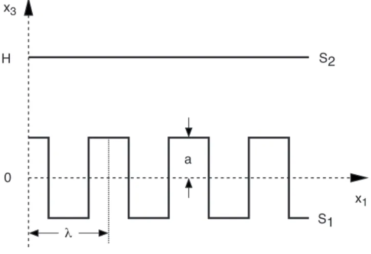
We consider the two interacting media as ﬁlling half spaces which are bounded by deformed surfacesS_α, α= 1,2. The deformations from a coplanar geometry of mean surface distance H are described by the height functionshα(x) withx the lateral surface coordinates, see Fig.B.1. The media are characterized by their complex dielectric functions_α(ω), respectively.

The gap between the media is assumed to be vacuum, i.e. (ω) = 1.

The free energyE of the photon gas in the gap between the two surfaces can be calculated from the imaginary time path integral for the electromagnetic gauge ﬁeldA^µ. In the absence

(21)

of media, the vacuum partition function Z0 is given by Z₀² =

[A^∗A]e⁻^SÊ^{Â^∗^,A^}, (B1.2) where we have introduced a complex valued gauge field which leads to a double counting of each degree of freedom. The reason for this will become clear below when we discuss the boundary conditions at the surfaces. Here, the functional integration runs over all fields which are defined on the whole space–time. The Euclidean actionS_E{A^∗, A}is the imaginary time version of the actionS{A^∗, A} of the electromagnetic field in Minkowskian space–time with coordinates X= (t,x) = (t,x, x₃),

S{A^∗, A} = −1 2

X

F_µν^∗ F^µν

(X)− 1 ξ

X

(∂_µA^∗^µ) (∂_νA^∗^ν) (X), (B1.3) where the ﬁrst term comes from the Lagrangian of the electromagnetic ﬁeldF^µν =∂^µA^ν−

∂^νA^µ and the second term results from the Faddeev–Popov gauge fixing procedure which assures that each physical field configuration is counted only once in the path integral over the gauge field. The parameterξ allows to switch between different gauges; all gauge invariant quantities calculated from this action like, e.g., the Casimir force, are independent of ξ. In the following, we will use the Feynman gauge corresponding toξ= 1. The coefficients in the action of Eq. (B1.3) differ by a factor of1/2from the conventional definition of the action for a real valued gauge field in order to obtain the correct photon propagator which in Feynman gauge reads Gµν = gµν/K² with momentum K = (ω,k), K² = KµK^µ = ω² −k² and Minkowskian metric tensor g_µν = diag(1,−1,−1,−1). The Euclidean action is obtained from Eq. (B1.3) by applying a Wick rotation to imaginary time which amounts to the transformations t → −iτ, ω → iζ and A⁰ → iA⁰, A^∗0 → iA^∗0 while the remaining components remain unchanged [108, 109]. Since this transformation corresponds to the changegµν → −δµν for the metric tensor, the Euclidean action in momentum space becomes

S_E{A^∗, A} = 1 β

∞ n=−∞

kA^∗^µ(ζn,k)G⁻¹_E_,µν(ζn,k)A^ν(ζn,k) (B1.4) where we allowed for a ﬁnite temperatureT by introducing bosonic Matsubara frequencies ζ_n = 2πn/β with β = 1/T. The Euclidean Green function is given by G_E,µν(ζ,k) = δµνG_E(ζ,k) with G_E(ζ,k) = (ζ² +k²)⁻¹. Note that here and in the following, integrals over momenta are always weighted with the factor (2π)⁻ⁿ, wherenis the dimension of the integral.

In the presence of the two media of mean surface separationHthe free energy (H–dependent ﬁnite part of the total energy) is obtained from a restricted partition function. The restrictions

(22)

are due to boundary conditions for the gauge field which are imposed by the dielectric properties of the media. It should be mentioned that there is an alternative, microscopic treatment of the Casimir force by considering the coupled system of fluctuating charges in the neutral materials and the gauge field. In the latter description, the Casimir interaction is mediated by the exchange of virtual photons. However, in our macroscopic formulation below we will look at the Casimir force as resulting from the perturbation of normal photon modes as opposed to the exchange of virtual quanta populating the unperturbed modes of the coupled system in unbounded space. Therefore, it is sufficient to derive the boundary conditions from classical electrodynamics which completely determine the normal mode structure in the presence of boundaries.

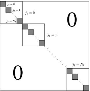
The restricted partition function will be defined for an auxiliary geometry which consists of three regions which are divided from each other by the infinitely large surfaces S₁ and S₂ which are assumed to be infinitesimally thin. All three regions are assumed to be vacuum space with the same velocity of light. As for the unrestricted partition function, the functional integral extends again over all gauge fields defined on the entire space–time. Below, we will show that the auxiliary geometry ”simulates” exactly the original geometry of two half spaces filled with dielectric materials (see Fig.B.1) when appropriate material dependent boundary conditions are defined on the infinitesimally thin surfacesS₁ andS₂. It turns out that there are three boundary conditions on each surfaceSα which we number by j= 1,2,3. Each of these conditions implies the vanishing of anon–locallinear combination of derivatives of the components of the gauge field. Since the boundary conditions will be non–penetrable, the two infinitesimally thin surfaces separate three regions with independent spectral problems.

One can imagine that the two half spaces are replaced by regions which are also bounded by two inﬁnitely large surfaces atx₃ → +∞ and x₃ → −∞ on which one imposes the same boundary conditions as onS₁ andS₂, respectively. Depending on the region the observer is located in, the boundary conditions ”simulate” a dielectric medium which occupies the entire space behind the surface. Thus, the restricted partition functions formally yield the sum of the energies of three similar spectral problems which diﬀer only by the mean surface distance.

The latter distance is sent to inﬁnity for the two outer regions which implies the vanishing of the corresponding Casimir energies. Thus, in this limit, which is always understood in the following, the restricted partition function yields exactly the ﬁniteH–dependent Casimir energy of the original geometry of Fig. B.1 The restricted partition functionZ(H) can be written as

Z(H)² =Z₀⁻²

[A^∗A]

αj

ζ_n

x∈R_α

δ

x∈S_α

L^αjµ(ζn;x,x)A^µ(ζn,x)

e⁻^S^E^{^A^∗^,A^}, (B1.5)

(23)

where we enforced the boundary conditions by inserting delta functions for all positions x on (flat) auxiliary surfaces R_α which are placed at x₃ = ±L with sufficiently large L so that the surfaces Sα are located between them, see Fig. B.1 The final result for the force between the media should (and will) be independent of L. The differential operators L^α_jµ depend via both the dielectric function_α and the normal vector nˆα on the surface indexα.

Their actual form will be computed below. The interaction (Casimir) free energy of the two surfaces S_α is given by

E(H) =−1 β ln

Z(H)Z_∞⁻¹(H)

, (B1.6)

whereβ = 1/T is the inverse temperature. Z_∞ is the asymptotic limit of Z for H→ ∞ so that E is measured relative to two surfaces which are inﬁnitely apart from each other. The Casimir force per unit area A between the surfaces is then given byF/A=−∂_HE/A.

1.1 Boundary conditions

In this section, we will derive the boundary conditions at the surfaces of the dielectric media.

The boundary conditions are based on the optical extinction theorem of Ewald [41] and Os- een [94], see also [17]. This theorem states that part of the electromagnetic field produced by the molecular dipoles inside a medium exactly cancels the incident field, while the remainder propagates according to Maxwell’s equations in continuous media. Ewald and Oseen proved the theorem for crystalline media and amorphous, isotropic dielectrics, respectively, using an approach based on classical molecular optics. Later, Born and Wolf extended the theorem to more general classes of materials [17]. A relationship between the extinction theorem and the Lifshitz theory of dispersion forces for continuous media has been pointed out by Milonni and Lerner [79]. They use the fact that the extinction theorem permits a reduction of the multiple scattering problem for the molecular dipoles to the solution of the wave equation for the gauge fieldA^µ with appropriate boundary conditions. From this they conclude that the extinction theorem shows that the macroscopic Lifshitz theory for continuous media cor- rectly accounts for all multiple scattering non–additive contributions to the force between flat surfaces. We will demonstrate that these concepts are useful to describe the interaction of even deformed surfaces.

We will use an (equivalent) reformulation of the extinction theorem as a non–local boundary condition which enforces the laws of reflection and refraction at the surfaces of the interacting media. Our derivation of the boundary conditions follows closely the approach outlined in [75]. We start with the common problem of finding solutions of Maxwell’s equations in the presence of a single interface separating two half spaces of materials with different dielectric functions. We assume that one half space is filled with a dielectric material described by(ω)

Casimir Forces and Geometry

Contents

A Introduction

B Casimir interaction between dielectric materials

ε

(ω) ε

(ω)