EPISTASIS, SHAPES & EVOLUTION M

& EVOLUTION

M ^ASTER ’ ^S T ^HESIS

000

100 110

101 010

011 110

000

000

101 011 110

101 111

011 110

000

001 011

000 001

010

100

101 111 011 110

M ALVIKA S RIVASTAVA

Institute for Biological Physics University of Cologne

D

2018

Second Corrector:

Prof. Dr. Thomas Wiehe

The figure on the cover page depicts type 1 triangulation of the three locus

Genotope. The fitness landscape that imposes this triangulation has shape 2.

Along with being consequential for evolution, epistasis is also quite preva- lent in nature. Thus, it is important to study it. Till date, there exist many methods of inferring epistasis from experimental and theoretical fitness land- scapes. The theory of shapes of fitness landscapes is another addition to that list. In this thesis, the shape theory of fitness landscapes is first introduced and then compared to pre-existing methods of gauging epistasis. From such a comparison for 3 locus landscapes, it turns out that landscapes of different interaction types differ in ruggedness, number of reciprocal sign epistasis mo- tifs and presence of higher order epistasis. Next, the applicability of shapes in studying empirical fitness landscapes is explored. Here the theory proves to be useful because the additional tests suggested by the Markov basis fur- ther corroborate the diminishing returns epistasis hypothesis, especially for the β -lactamase landscape with synonymous mutations. Moreover, the trian- gulation of the landscape of large effect mutations has a particular genotype as vertex of every tetrahedra in the triangulation, indicating the presence of that genotype in all fittest populations. Finally, the effect of the shape on the evolutionary dynamics is discussed. For two locus landscapes, the equilibra- tion time of the mutation-selection dynamics has a sharpness exactly at the transition point between the two shapes. Further, it was found that Eshel and Feldman’s results regarding the advantage of recombination in two locus permutation invariant landscapes can be extended to three locus landscapes.

It turns out that in three out of the six shapes of permutation invariant land-

scapes, recombination is "advantageous", while in the other three, it is "dis-

advantageous". This extensive analysis of its applicability indicates that the

shape theory offers useful insights while studying empirical landscapes, how-

ever additional constraints are needed to predict evolution on landscapes of

different shapes.

Hiermit versichere ich an Eides statt, dass ich die vorliegende Arbeit selb- stständig und ohne die Benutzung anderer als der angegebenen Hilfsmit- tel angefertigt habe. Alle Stellen, die wörtlich oder sinngemäßaus veröf- fentlichten und nicht veröffentlichten Schriften entnommen wurden, sind als solche kenntlich gemacht. Die Arbeit ist in gleicher oder ähnlicher Form oder auszugsweise im Rahmen einer anderen Prüfung noch nicht vorgelegt wor- den. Ich versichere, dass die eingereichte elektronische Fassung der eingere- ichten Druckfassung vollständig entspricht.

Köln, April 2, 2019

Malvika Srivastava

First and foremost, I would like to express my deepest gratitude to my super- visor, Prof. Dr. Joachim Krug, for indicating the starting point of my thesis and then giving me the rare freedom and the accompanying opportunity to find my own path, for always giving useful inputs and for being extremely thoughtful and supportive throughout.

Next, I would like to thank all my group members and colleagues here–

Alex, Benjamin, David, Jonas, Lucy and Suman, for always being there to listen, talk and help. Lucy deserves a special mention for never failing to lift my spirits when they were flagging. I want to additionally thank Benjamin for always agreeing to debug Julia and translate German documents. I would also like to thank Lara Bössinger from the mathematics department, for I learnt more from her in 2 hrs than I learnt from textbooks in 2 months. And finally Nikhil, for always pushing me to improve and develop confidence in myself, by being my best friend and my harshest critic.

Last, but definitely not the least, I want to thank my family and friends in

India and elsewhere, who were yet just a phone call away. Especially, my par-

ents for their unwavering support and love– I can never thank them enough

for that, and my little sister Manya, who’s now old enough to help me under-

stand concepts from group theory. They make it all worthwhile.

1 Introduction 7

1.1 Forces of evolution . . . . 7

1.2 Fitness landscapes . . . . 7

1.3 Epistasis . . . . 10

1.3.1 Causes of epistasis . . . . 10

1.3.2 Measures of epistasis . . . . 10

1.4 Overview of the thesis . . . . 12

2 The shape theory 13 2.1 Mathematical preliminaries . . . . 13

2.2 Elements of the theory . . . . 16

2.2.1 The Genotope . . . . 16

2.2.2 Triangulations of the Genotope . . . . 16

2.2.3 Tools for triangulation . . . . 18

2.3 Examples of shapes . . . . 20

2.3.1 2 locus case . . . . 20

2.3.2 3 locus case . . . . 21

3 Shapes and their contemporaries 28 3.1 Applications of shapes . . . . 28

3.2 Shapes in comparison to graphs . . . . 29

3.3 Shapes in comparison to the Walsh spectra . . . . 30

3.4 Shapes in comparison to the γ measure . . . . 34

4 Application to empirical landscapes 36 4.1 Previous work . . . . 36

4.2 New results . . . . 38

5 Shapes and evolution: Mutation-Selection 44

5.1 Mutation-selection dynamics . . . . 44

5.2 Two locus case . . . . 45

5.3 Three locus case . . . . 55

6 Shapes and evolution: Recombination 58 6.1 Recombination . . . . 58

6.2 The evolution of recombination . . . . 60

6.2.1 Direct models . . . . 60

6.2.2 Indirect models . . . . 60

6.3 The effect of shapes . . . . 61

6.3.1 Two locus case . . . . 62

6.3.2 Three locus case . . . . 64

7 Final remarks 78 7.1 Conclusions . . . . 78

7.2 Future directions . . . . 80

Introduction

By attributing our existence to accident, and not design, evolution, both re- moves and adds meaning to life. On one hand, it strips the human race of its narcissism, while on the other, it makes life valuable, by highlighting its sheer improbability. Also, by offering explanantions for a variety of natural phenomena, evolution makes the world we see around us, a little less surpris- ing. So in short, evolution is the best answer we have to some of the most profound questions we have about ourselves and our surroundings. Moreover, evolution not only lends us perspective on our lives, it also serves as a guide to solving complex problems– as was testified by the recent Nobel prize in chemistry, that was awarded for using directed evolution in the lab to develop useful chemicals [1].

1.1 Forces of evolution

In a nutshell, evolution is driven by the forces of selection, mutation, recom- bination, genetic drift and migration. While mutation, recombination and mi- gration are responsible for introducing diversity on which selection can act, genetic drift accounts for the inevitable fluctuations in the dynamics of finite populations. In this thesis, only the forces of selection, mutation and recombi- nation are included and the population size is considered to be infinite, which means that the population dynamics is deterministic.

1.2 Fitness landscapes

Evolutionary processes span many length and time scales. Even events oc-

curring on small scales, for instance mutation in a single base pair, can have

Figure 1.1: The one, two, three, four and six dimensional Hamming spaces.

Source: [2]

cascading effects on the overall fitness of an organism [3]. So a natural ques- tion that arises is how can we study this multi-scale process? This is where the concept of fitness landscapes comes into the picture.

The term fitness can mean different things in different contexts [4]. While it typically refers to the fecundity of an organism, it could also refer to the viability in studies of age structured populations or the minimum inhibitory concentration (MIC) in studies of antibiotic resistance. Regardless of its def- inition, fitness of an organism is co-determined by its DNA sequence or its genotype and the environment in which it evolves. This means that for a con- stant environment, there exists a map from the genotype of an organism to its fitness.

The genotype of a haploid organism can be simply modelled as a sequence of a fixed number of sites L, with a fixed number of alleles a, at each site. Each site can represent, for example, a nucleotide (i.e. A,G,T or C ⇒ a = 4) or even an entire gene. The genotype space G, is then the set of all possible sequences of length L that can be formed by combining the a alleles at each site and

| G | = a

. Further, a metric can be defined for the genotype space in terms of

the number of sites at which two sequences differ. In the case of a alleles, the

genotype space can be mapped to the L dimensional, a-allelic Hamming space ( H

) [5] and the metric then is the Hamming distance

d( σ , γ ) =

L

X

i=1

(1 − δ

) (1.1)

where σ and γ are sequences of length L , δ

is the Kronecker delta function and σ

, γ

are the alleles at the ith sites on the sequences σ and γ respectively.

In this thesis, the discussion will be confined to bi-allelic sequences, where the L dimensional binary Hamming space H

can be represented by the ver- tices of the L-dimensional hypercube (figure 1.1).

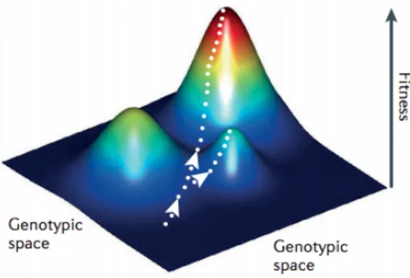
Figure 1.2: An illustration of a fitness landscape. The white arrows represent evolutionary trajectories. Source:[6]

With that we have all three "ingredients" [7] required to define a fitness landscape, namely, a configuration space i.e. G, a notion of distance between the elements of the space i.e. d( σ , γ ) and a map from every element σ of G to the fitness, F( σ ) ∈ R. A fitness landscape is then defined as F : G → R.

Figure 1.2 shows a fitness landscape, like it was first imagined by Sewall Wright [8]. Wright himself realized that it is an inadequate representation of the true higher dimensional picture because it constrains the genotype space to be only two dimensional.

Theroetical fitness landscapes can be modelled in several ways [6]. Fol- lowing are two of the most commonly used models:

• HoC model: The simplest model is called the House of Cards (HoC)

model [9] and it assumes every fitness value to be an independent iden-

tically distributed (i.i.d) random variable.

• NK model: The NK model generates landscapes with tunable rugged- ness and was first introduced in [10]. Here, N stands for the number of loci in the sequence (=L) and each locus interacts with K-1 other loci.

Within each set of the K interacting loci, fitness contributions are as- signed at random to the 2

possibilities. The HoC model is a limiting case of the NK model when K=N.

1.3 Epistasis

Epistasis, to quote Weinreich et al. [11], is the "surprise at the phenotype when mutations are combined, given the constituent mutations’ individual ef- fects". This just means that mutations don’t have independent effects. Rather, their effects depend upon the background sequence on which they occur. This makes epistasis highly consequential for evolution. In fact, many studies have already recognised the importance of epistasis for adaption, evolutionary pre- dictability and the evolution of sexual reproduction [12, 13, 6]. Epistasis has also been linked to the topography of fitness landscapes [14, 15], which de- termines the accessibility of adaptive walks in sequence space. Moreover, epistasis is highly prevalent in nature and empirical fitness landscapes are known to be topographically complex [6]. This makes its inclusion in theoret- ical studies necessary. Lastly, the recent hypothesis that complex traits may be omnigenic [16] and that the effect of "core" genes also depends upon all the "peripheral" genes, just highlights the presence of epistasis between these genes.

1.3.1 Causes of epistasis

In [17], possible proximate and evolutionary causes of epistasis are discussed.

In the past, people have used metabolic models and the concept of pleiotropy

and robustness to predict and explain epistasis. In theoretical studies, epis-

tasis has also been thought of as a dynamic variable that is subjected to evo-

lutionary forces of selection, drift, mutation and recombination. The motiva-

tion for that is most probably Malmberg’s [18] experimental system where re-

combination alleviated epistasis between beneficial alleles. However, despite

many forward steps, the origin and dynamics of epistasis are still enigmatic.

1.3.2 Measures of epistasis

Unidimensional epistasis

One can either study unidimensional epistasis or multidimensional epista- sis [19]. The unidimensional study entails looking at the mean log fitness as a function of the number of mutations. Deviations from linearity is then interpreted as epistasis. Due to the ease of measurements, most experimen- tal studies use the unidimensional definition of epistasis. However, it fails to provide a complete picture of the underlying interactions because despite the presence of interacting loci, unidimensional epistasis can be zero. This is where multidimensional epistasis comes to use.

Multidimensional epistasis

By considering interactions between all possible combinations of loci, multidi- mensional epistasis provides crucial information about the number of peaks and the accessibility of fitness landscapes. It can be classified into 2 types:

1. Pairwise epistasis, as the name suggests, refers to epistasis between loci pairs. It can further be classified into a) Magnitude and b) Sign epis- tasis, based on whether the effect of a mutation has a different magni- tude on a different background or whether it has an altogether different sign. A special case of sign epistasis is called reciprocal sign epistasis, wherein the sign of the mutational effect of either mutation changes in the presence of the other.

2. Higher order epistasis refers to interactions between more than 2 loci and it has been relatively less studied [11]. It essentially means that only knowledge of the fitnesses of the wild type, the single mutants and the double mutants is not enough to determine the rest of the fitness landscape. Like pairwise epistasis, higher order epistasis can also be classified into sign and magnitude epistasis.

In order to assess its ubiquity, Weinreich et al. [11] analysed 14 pub-

lished fitness landscapes and found that in nearly every case, the mean

magnitude of higher order contributions were larger than or equal to

the pairwise effects, implying that higher order epistasis is quite preva-

lent in nature. More recently, abundance of higher order epistasis was

also found in [20] and its indispensibility in determining evolutionary

trajectories was identified in [21, 22]. However, despite that, there is no

unique way of extracting information or classifying landscapes based on these interactions.

Since fitness landscapes with multiple loci have complex high dimen- sional structures, it is important to be able to characterize them based on simpler and preferably scalar measures. The following ways to study and classify higher order epistasis exist in the literature:

• For combinatorially complete fitness landscapes, the Walsh coeffi- cients [23] can be obtained by a linear transformation of a vector containing the fitness values of all the genotypes. The first order Walsh coefficients represent the individual mutational effects av- eraged over all possible backgrounds, the second order coefficients represent pairwise epistasis averaged over all backgrounds and the higher order coefficients have similar interpretations.

• In [24] and [22], Crona et al. showed that higher order epista- sis can also be inferred from fitness graphs which are basically di- rected acyclic hypercube graphs. What makes this interesting is that their analysis requires only the partial order of fitness values and not the actual values themselves. From fitness graphs, one can also extract indirect measures of epistasis, such as the number of peaks, the fraction of sign/reciprocal sign epistasis motifs etc.

• Another measure based on the correlation of mutational effects was developed in [25]. They defined an epistasis measure γ = Cor(s(g),s(g

)), where s( g

) is the fitness effect of a mutation oc- curring at site i on the genotype g and g

represents neighbouring genotypes of the genotype g. Like fitness graphs, this method can also be employed to incomplete fitness landscapes, although the error in the estimate of γ increases with the fraction of unknown fitness values. But unlike fitness graphs, it can also be used to in- fer magnitude epistasis. Further, it proves to be different from the non-linear part of the Walsh spectrum [14] because it gives more weight to higher order epistasis than pairwise epistasis.

• Last, but hopefully not the least, is the shape theory of fitness land-

scapes [26]. It is also the first study that considered higher order

epistasis to be important. Herein, the authors identified pairwise

and higher order epistasis tests (i.e. circuits and Markov bases)

that should be relevant for classifying fitness landscapes based on

the kind of epistatic interactions that they exhibit. Studying the

usefulness of these epistasis tests and the classification prescribed

by the authors, in comparison to the other measures, comprises one of the main motives of this thesis.

1.4 Overview of the thesis

To summarize, epistasis strongly affects both the static properties of fitness landscapes, like its ruggedness, and the dynamic properties of populations evolving on these landscapes. Although the fitness landscape is a coarse grained concept, that glosses over several intermediate levels, a lot can still be learnt from it because it’s possible to extract information about mutational interactions from it. However, for multi-loci (L > 2) landscapes, there is no unique way of doing this. Furthermore, it is also of interest to be able to clas- sify landscapes based on these interactions. The hope that landscapes with similar interactions will show similar static properties and population dynam- ics is implicit in the attempts to classify landscapes. This very hope will drive the discussion in the following chapters and the primary focus will be on the recently developed shape theory of fitness landscapes.

The organisation of the next chapters is as follows: In chapter 2, the geo-

metric theory of fitness landscapes is introduced. Then in chapter 3, shapes

are compared to other ways of classifying epistatic fitness landscapes. In chap-

ter 4, the shape theory is applied to some empirical fitness landscapes, in or-

der to see if some additional insights are gained from doing so. In chapter

5, the focus is on mutation-selection dynamics of populations on landscapes

with different shapes. Next, the question of evolution of recombination, in the

context of the shape theory, is addressed in chapter 6. Finally, in chapter 7,

conclusions and the future directions are discussed.

The shape theory

The shape theory of fitness landscapes was developed in [26]. The motiva- tion of the authors was to highlight the underlying combinatorial geometry of fitness landscapes. The basic idea is that epistatic interactions between mul- tiple loci can take place in a finite number of ways. The regular triangulations of the Genotope, encode these finite possibilities of interaction. Therefore, to quote the authors, “The biological problem of studying the genotype interac- tions for a fitness landscape is thus equal to the combinatorial problem of finding the shape of the fitness landscape...". However, to be able to fully understand and appreciate this statement, some mathematical foundation is built in the first section.

2.1 Mathematical preliminaries

In the following: For n points v

, v

, ..., v

in R

A := £

v

v

... v

¤

∈ R

Definition 2.1.1. An affine space is {x ∈ R

: B · x = b} where B is a m × n matrix and b ∈ R

.

Definition 2.1.2. An affine combination of a set of points {v

} equals P λ

· v

where P λ

= 1 and λ

∈ R ∀ i

Definition 2.1.3. A set of points is said to be affinely independent if no point in the set can be expressed as an affine combination of all the other points in the set. Else the points are affinely dependent.

Definition 2.1.4. A convex combination of a set of points is an affine combi-

nation with λ

≥ 0 ∀ i .

A conv(A)

Figure 2.1: The convex hull of a given point configuration.

Definition 2.1.5. The convex hull of a set of points A is the set of all convex combinations of the points. It is denoted as conv(A) and is illustrated in figure 2.1.

Definition 2.1.6. There are two equivalent

ways of defining a polytope:

1. A (V-) polytope is the convex hull of a finite set of points.

2. An (H-) polytope is the intersection of half spaces

that must be bounded.

Definition 2.1.7. An n-simplex is the convex hull of n + 1 affinely independent points, e.g. a 0-simplex is a point, 1-simplex is a line, 2-simplex is a triangle and 3-simplex is a tetrahedron.

Definition 2.1.8. A polyhedral subdivision of a point configuration A is a set of polytopes C such that:

1. If c ∈ C, each face of c belongs to C (closure property) 2. The union of c is equal to conv(A) (union property)

3. For c, c

∈ C and c 6= c

, the intersection of c and c

doesn’t contain any interior points of c or c

. (intersection property)

Definition 2.1.9. A polyhedral subdivision is a triangulation if all the poly- topes in C are simplices.

1Main Theorem of Polytope Theory[27]

2Any hyperplane~^a·~^x=binR^d defines two half-spaces~^a·~^x≤band~^a·~^x≥b

(a) The poset of subdivisions (b) The secondary polytope

Figure 2.2: Subdivisions of a pentagon.

Definition 2.1.10. A regular triangulation is one that can be induced by a lifting construction (see figure 2.3), which in our case is a fitness landscape.

Definition 2.1.11. A GKZ (Gelfand, Kapranov and Zelevinsky) vector of a triangulation ∆ of A is the vector:

φ

: = X

(vol( τ ) : τ ∈ ∆ ^{and i} ∈ τ ) ~ ^e

∈ R

(2.1) where, vol( τ ) is the normalised volume of the simplex τ , i.e. the absolute value of the determinant of A

divided by the greatest common divisor (g.c.d.) of the maximal minors of A.

Definition 2.1.12. A secondary polytope of a given point configuration A is the convex hull of the GKZ vectors corresponding to the triangulations of A. In simpler terms, a secondary polytope is a polytope whose vertices are in bijection with regular triangulations of A (see figure 2.2 b) ).

Actually, the poset

of regular polyhedral subdivisions of a point set A equals the face poset

of the secondary polytope of A. Thus, triangulations are minimal elements in the poset of subdivisions.

Definition 2.1.13. If a subdivision is only refined

by triangulations then it is refined by exactly two of them. These two triangulations are then said to differ by a bistellar flip.

3with partial ordering induced by refinement

4This is the set of all faces of a polytope ordered by set inclusion.

5If setsS={S1...S_l}andT={T1...Tm}are two subdivisions of conv(A), then T is a refine- ment of S if∀j, 1≤j≤m,∃i, 1≤i≤lsuch thatTj⊆Si

These flips constitute the next to minimal elements in the poset of polyhe- dral subdivisions of A [28]. The poset of subdivisions of a pentagon is shown in figure 2.2 a). Essentially, flips are the minimal possible changes in the shape and are detected by minimal affine dependences in the point configu- ration. An interesting result is that the graph of triangulations of n points in convex position in R

is connected [29]. This means one can go from one triangulation to any other by means of repeated number of flips.

2.2 Elements of the theory

2.2.1 The Genotope

As described before, the genotype space G is a set of a

points in R

.

Definition 2.2.1. The Genotope Π

is the convex hull of the genotype space.

The convex hull of any finite point configuration is nothing but a convex polytope. In this case, the vertices of the convex polytope represent the a

possible sequences. For instance, in the 2 loci bi-allelic case, the Genotope is simply a square with vertices (0,0), (0,1), (1,0), (1,1).

Definition 2.2.2. An allele frequency vector ~ ν for a bi-allelic population is an L-dimensional vector and its ith entry ( ν

) represents the fraction of the population that has the mutated allele 1 at its ith site.

The vertices of the Genotope can also be viewed as the allele frequency vectors of homogeneous populations composed of only one genotype. Then, each point enclosed by the Genotope represents the allele frequency vector of a heterogeneous population that is composed of several genotypes. Thus, the Genotope is basically a set of all possible allele frequency vectors. Note that the concept of the Genotope can also be extended to diploids.

2.2.2 Triangulations of the Genotope

The Genotope is merely a set of all possibilities. Which possibilities get re- alised in nature is governed by evolutionary forces. The structure of the fit- ness landscape encodes one such force, which is the force of natural selection.

Applying the fitness landscape map to the vertices of the Genotope amounts

to lifting the configuration to one higher dimension, by raising each vertex by

an amount equal to the fitness of the genotype that is represented by that

vertex. The convex hull of these raised vertices is also a convex polytope.

R ^d R

Figure 2.3: An example of a lifting construction that induces regular triangu- lations, although in this case the lower surface (instead of the upper surface) of the higher dimensional polytope is projected. Adapted from: [28]

The projection of the upper surface of this higher dimensional polytope on the Genotope then gives rise to a triangulation of the Genotope.

This can be formalised as follows: We can extend the definition of the fit- ness landscape to also assign a fitness value to every allele frequency vector lying inside the Genotope. This can be done by assigning the maximum fit- ness that a population with the given allele frequency vector can have. This new continuous fitness landscape is a piece-wise linear convex function and the domains of linearity of this function are actually the simplices in the tri- angulation.

The number of possible triangulations of a given Genotope is finite. For 2 loci, there are 2, for 3 loci there are 74, while for 4 loci, there are already 87959448. Fitness landscapes that induce the same triangulation are said to have the same shape.

Definition 2.2.3. The shape of a fitness landscape is the triangulation of the Genotope that is induced by it.

It will become obvious later that landscapes of the same shape have simi- lar epistatic interactions between their loci.

Another important information provided by the shape is that the vertices

of the simplex to which the allele frequency vector of a population belongs,

are the genotypes that will be present in the maximally fit population,

given that the allele frequency vector remains fixed during the dynamics. This

is not obvious at first glance, but it can be proved using results from linear

000 001 010

100

101 111 011

110

(⌫1, ⌫2, ⌫3)

Figure 2.4: A triangulated Genotope

programming

. For example, for the allele frequency vector shown in figure 2.4, the maximally fit population will contain the genotypes 000, 011, 110 and 010. This is a useful fact for dynamics like recombination in which the allele frequency vectors remain unchanged. This also implies that the ith entry of the GKZ vector represents the probability that the corresponding genotype occurs in fittest populations conditioned upon allele frequency vectors.

2.2.3 Tools for triangulation

Testing whether a set of subsets of a point configuration comprises a triangu- lation of that point configuration, is a non-trivial computational problem [28].

This is where circuits and Markov bases come to use. While circuits are com- binatorial tools that lead to a fully algorithmic definition of a triangulation, Markov bases exploit the rich link between algebraic geometry and triangu- lations to construct triangulations. Moreover, these two tools for constructing triangulations reveal patterns of multidimensional epistasis exhibited by the fitness landscape.

In order to better explain these concepts, one needs to introduce the fol- lowing others:

• Additive epistasis can be measured by looking at linear combinations of genotype fitnesses. Certain sets of these linear combinations form inter- action coordinates and both magnitude and sign of these coordinates are relevant when examining the landscape of a biological organism. Now,

6Namely, the fundamental theorem of linear programming, which states that the extremal values of a linear function over a convex polytope are attained at its vertices.[30]

Figure 2.5: A cartoon illustrating the map ρ . ∆

represents the probability simplex corresponding to the genotype space G.

any fitness landscape can be represented as a vector ~ ^w ∈ R

, where | G | is the number of genotypes. Let L

⊂ R

such that every ~ ^w ∈ L

is com- pletely non-epistatic, i.e. there exists an affine-linear form on the Geno- tope, whose values are w

at the vertices ⇒ L

= { ~ ^{w :} ~ ^v · G ~ + c = w

∀ G} ~ where ~ ^v · + c is an affine linear form on Π

, G ~ represents a vertex of Π

and w

is the corresponding fitness of vertex _G. ~

Definition 2.2.4. The interaction space is then defined as the dual vector space of the quotient of R

modulo L

i.e. I

= ( R

/L

)

. Thus, elements of I

are linear forms that vanish on L

.

Definition 2.2.5. Finally, circuits are linear forms that (redundantly) span the interaction space and have non-empty but minimal support.

The number of circuits is usually larger than the dimension of I

(d(I

) = 2

− L − 1) but is bounded above by ¡

d(I_G)−1

¢ .

• Let’s define ρ to be a map that takes population frequency vectors (that lie in a 2

− 1 dimensional simplex) to their corresponding allele fre- quency vectors (that are contained in the Genotope) i.e. ρ : ~ ^x 7→ ~ ν , where

~ ^x = (x

, ...., x

) and ~ ν = ( ν

, ...., ν

). This map is clearly not a bijec- tion and therefore the pre-image of any ~ ν ∈ Genotope ( Π

) is ρ

( ~ ν ) = { ~ ^{x :} ρ ( ~ ^x) = ~ ν }. This is illustrated in figure 2.5. The dimensions of ρ

( ~ ν ) = 2

− L − 1 = d(I

). ρ when written as a matrix, turns out to be the matrix whose columns are the vertices of the Genotope.

For instance, in the 2 loci case:

ρ =

· 0 0 1 1 0 1 0 1

¸ ,

while in the 3 locus case:

ρ =





0 0 0 0 1 1 1 1 0 0 1 1 0 0 1 1 0 1 0 1 0 1 0 1



.

• The integral kernel of ρ i.e. ker

( ρ ) = { ~ k : ρ ( ~ _{k) = 0} ∩ Z}

defines the interaction space for the genotypes. The Markov basis or the circuits are a non-independent basis for the interaction space. I will henceforth omit the subscript of ker

( ρ ), however unless otherwise stated, ker( ρ ) will still refer to the integral kernel and not the entire kernel.

• A more concrete definition of Markov bases exists in the context of Toric ideals.

Definition 2.2.6. A Toric ideal, I

= 〈 p

− p

: ρ ( ~ ^u) = ρ ( ~ v)〉, where, p

= p

p

... p

represents a monomial in n variables p

, p

...p

and 〈 P 〉 represents the ideal

generated by a set of polynomials P . In other words, a Toric ideal is the ideal generated by binomials of the form p

− p

where ~ ^{u and} ~ ^v satisfy the above mentioned property.

Definition 2.2.7. A finite set of binomials, with the above stated prop- erty, that generates the Toric ideal I

is called a Markov basis for the Toric ideal, i.e. if I

= 〈 {x

− x

: ρ ( ^m ~

) = ρ ( ^m ~

)}〉 then, the finite set of all ^m ~ = ^m ~

− ^m ~

is called a Markov basis.

• From this definition, it can be seen that ^m ~ ∈ ker( ρ ) ∵ ρ ( ^m ~

) = ρ ( ^m ~

) ⇒ ρ ( ^m ~

− ^m ~

) = ρ ( ^m) ~ = 0. Therefore, a Markov basis can alternatively be defined as a subset B of ker( ρ ) that satisfies the following conditions:

1. If ∀ ~ ^u, ~ ^{v satisfying} ρ ~ ^u = ρ ~ ^v, ∃ { ^m ~

}

=1

, such that ~ ^u + P

i

^m ~

= ~ ^{v and} 2. ∀ j satisfying 1 ≤ j ≤ l, ~ ^u + P

i=1

^m ~

≥ 0

If conditions 1. and 2. are met, then B is a Markov basis and every m ∈ B is called a move. Markov basis can be used to do Monte-Carlo simula- tions. For example, in our context, adding a move to a probability vector will give a new probability vector with the same allele frequency vector as the original probability vector. This way, one can hop in the subset of the probability simplex which maps to a particular allele frequency vec- tor. Further, with some pre-knowledge about the stationary probability distribution, one can get the probability of taking a certain step. This can then be used to compute equilibrium averages of quantities.

• Lastly, circuits measure additive epistasis while Markov basis elements measure multiplicative epistasis.

7For more information on polynomial rings and ideals, see[27]

2.3 Examples of shapes

2.3.1 2 locus case

Figure 2.6: Possible shapes for 2 loci landscapes. Landscapes with e < 0 have the shape shown in the left most figure, while those with e > 0 have the shape shown in the right most figure. The central figure corresponds to non-epistatic landscapes that do not triangulate the Genotope and hence have no shape.

Triangulations for the 2-loci Genotope are almost trivial because there is only one possible interaction between the 2 loci. This interaction is measured by the circuit: e = w

+ w

− w

− w

. This circuit gives rise to two shapes that are shown in figure 2.6.

The shape of a two locus fitness landscape is not very informative about its topography because the probability of exhibiting a particular type of sign epistasis (either simple, reciprocal or no sign epistasis) remains independent of the shape of the landscape. This is because for example:

P (reci) = P(reci | shape1)P(shape1) + P (reci | shape2)P(shape2) (2.2) where, P (reci) represents the probability of having reciprocal sign epsiatsis.

Now, for HoC fitness landscapes P(shape1) = P(shape2) = 0.5.

⇒ P (reci) = 0.5 · P(reci | shape1) + 0.5 · P(reci | shape2) (2.3) Now, P(reci | shape1) = P(reci | shape2) because the two shapes differ merely by labelling. Exchanging the labels w

←→ w

and w

←→ w

exchanges the shape as well.

⇒ P(reci | shape) = P(reci) (2.4)

All we can know from the shape is the location of the two peaks, given

that there is reciprocal sign epistasis. This however is not surprising because

in the 2 loci case, shapes are distinguished only by the sign of a circuit mea- suring magnitude epistasis. Therefore, the more useful knowledge about sign epistasis (and thus the number of peaks) is not contained in the shapes of the 2-loci landscape.

2.3.2 3 locus case

As previously mentioned, there are 74 possible triangulations for the bi-allelic, 3 locus case. These belong to 6 symmetry classes or interaction types. I will explain why there are 74 shapes and 6 types, through a small story about Newton polytopes and hyperdeterminants. This story has been completely bor- rowed from [31].

• The Newton polytope N(G) of a polynomial G is the convex hull of the exponent vectors of the monomials which appear in the expansion of G.

• The hyperdeterminant of a 2 × 2 × 2-tensor, D

is an irreducible poly- nomial in eight variables with twelve monomials of degree four and is called a tangle in physics literature. Note that it is the higher dimen- sional analog of the determinant of a 2 × 2 matrix which is the polynomial D

= x

x

− x

x

in four variables.

• N(D

) is the convex hull in R

of the six rows of the following matrix:



















1 0 0 1 0 1 1 0 0 1 1 0 1 0 0 1 2 0 0 0 0 0 0 2 0 2 0 0 0 0 2 0 0 0 2 0 0 2 0 0 0 0 0 2 2 0 0 0



















This is because the exponents of these monomials are vertices of N(D

).

This makes them extreme monomials. The exponents of the remaining 6

monomials lie in the interior of N(D

) and do not contribute to the con-

vex hull. The f-vector records the number of faces of dimension 0,1,2...d-

1 and f (N(D

))=(6,14,16,8), meaning that N(D

) has 6 vertices, 14

edges, 16 2-dimensional faces and 8 3-dimensional faces.

• A final relevant character in the story is the principal determinant of the 3-cube i.e.

E

= D

· (x

x

− x

x

) · (x

x

− x

x

) · (x

x

− x

x

) · (x

x

− x

x

) · (x

x

− x

x

)· (x

x

− x

x

)·

x

· x

· x

· x

· x

· x

· x

· x

. This is a polynomial of degree 24 with 231 monomials out of which 74 are extreme monomials. It turns out that N(E

) is the secondary polytope of the 3 cube. It is 4-dimensional and its f-vector is (74,152,100,22).

Further, its 74 vertices are in bijection with the regular triangulations of 3 cube. Moreover, the symmetry group of the 3-cube is the Weyl group B

of order 48 and it turns out that the 74 extreme monomials come in 6 orbits

. And that solves the mystery of 74 shapes and 6 types!

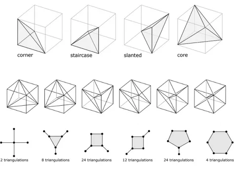
The tight spans of the 6 types of shapes are shown in figure 2.7.

The following is a brief description of the types:

1. Type 1 contains 2 shapes that divide the cube into five tetrahedra, one central tetrahedron of normalized volume two surrounded by four of nor- malized volume one.

2. Type 2 contains 8 shapes that are generated by slicing off the three vertices adjacent to a fixed vertex and cutting the remaining bipyramid into three tetrahedra.

3. Type 3 contains 24 shapes that are generated by picking a diagonal and two of the other six vertices that are diagonal on a facet, and slicing them off.

4. Type 4 has 12 shapes which are indexed by ordered pairs of diagonals.

The end points of the first diagonal are sliced off, and the remaining octahedron is triangulated using the second diagonal.

5. Type 5 has 24 shapes that are indexed by a diagonal and one other vertex which is sliced off, and the remaining polytope is divided into a pentagonal ring of tetrahedra around the diagonal.

6. Type 6 has 4 shapes that are indexed by the diagonals. The cube is

divided into a hexagonal ring of tetrahedra around the diagonal.

Figure 2.7: Top to bottom: The types of tetrahedra that appear in the trian- gulation of the 3 cube, the six types of triangulations of the 3 cube and the tight spans of the 6 types– the vertices represent the tetrahedra in the tri- angulation and two vertices are connected if the tetrahedra share a common triangle. Source: [32]

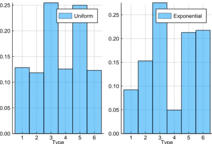
The distributions of shapes and types of HoC fitness landscapes are shown in figures 2.9 and 2.8 for the uniform distribution and the exponential distri- bution. As is evident, the distribution depends upon the probability distribu- tion from which the fitness values are assigned.

For uniformly distributed HoC landscapes, each shape of a particular type is equally likely to occur. This is because shapes of a particular type can be obtained from one another by re-labelling of the indices. Moreover, one could naively expect each type to be equally likely to occur. This however cannot be the case because the probabilities would not be normalised any more. Type 3 and type 5 are actually the most abundant types with an abundance of ap- proximately 25% each. The other four types have an abundance of nearly 12.5% each. Another way to obtain the shape distribution and verify the re-

8For a group G that acts on a set X, the orbit of every x∈X is Orbx={g.x:g∈G}⊂X.

sults obtained by triangulating the fitness landscape is to look at the circuits.

The 20 circuits for the 3-loci case are as follows:

a := w

− w

− w

+ w

b : = w

− w

− w

+ w

c : = w

− w

− w

+ w

d : = w

− w

− w

+ w

e : = w

− w

− w

+ w

f : = w

− w

− w

+ w

g := w

− w

− w

+ w

h := w

− w

− w

+ w

i : = w

− w

− w

+ w

j : = w

− w

− w

+ w

k : = w

− w

− w

+ w

l : = w

− w

− w

+ w

m : = w

+ w

+ w

− w

− 2w

n := w

+ w

+ w

− w

− 2w

o := w

+ w

+ w

− w

− 2w

p : = w

+ w

+ w

− w

− 2w

q : = w

+ w

+ w

− w

− 2w

r : = w

+ w

+ w

− w

− 2w

s : = w

+ w

+ w

− w

− 2w

t := w

+ w

+ w

− w

− 2w

Circuits a-f check for pairwise epistasis, g-l for marginal epistasis between two pairs of loci and m-t for three way epistasis in relation to total pairwise epistasis.

The shapes are characterized by the sign pattern of a selected number of circuits. For instance, for a fitness landscape to have shape 1, circuits t, q, o and m must be positive. Thus, the shape abundances can also be com- puted by looking at probabilities that a random landscape will have a circuit sign pattern that characterises that particular shape. One more motivation for computing the abundances differently was to check if the abundances are rational numbers (i.e. 1/4 and 1/8).

Since circuits are nothing but linear combinations of i.i.d random vari-

ables, one can estimate the probability of obtaining a set of 8 random vari-

1 2 3 4 5 6 0.00

0.05 0.10 0.15 0.20 0.25

Type Uniform

1 2 3 4 5 6

0.00 0.05 0.10 0.15 0.20 0.25

Type Exponential

Figure 2.8: The relative abundances of the 6 types for HoC landscapes gener- ated from a uniform distribution and an exponential distribution.

ables that satisfy a certain circuit sign pattern by computing the volume of the polytope bounded by hyper-planes given by the circuit sign pattern, e.g.

P(shape1) = Z

0

...

Z

0

Π

^dw

Θ ^(t({w

})) Θ ^(q({w

})) Θ ^(o({w

})) Θ ^(m({w

})) (2.5) These integrals were easily computed by using the Monte-Carlo method.

The resultant abundances matched the previously obtained ones (shown in table 3.1), however it still could not be ascertained whether these abundances were rational numbers.

Finally, figure 2.10 summarises the GKZ vectors, defining circuits and

neighbours on the secondary polytope of all the 74 shapes.

0 20 40 60 0

100 200 300 400 500 600

Shape

Frequency

Type 1 Type 2 Type 3 Type 4 Type 5 Type 6

(a) Shape distribution for HoC landscapes with uniformly dis- tributed fitness values.

0 20 40 60

0 100 200 300 400 500

Shape

Frequency

Type 1 Type 2 Type 3 Type 4 Type 5 Type 6

(b) Shape distribution for HoC landscapes with exponentially dis- tributed fitness values.

Figure 2.9

Figure 2.10: All 74 shapes of the 3-cube with their GKZ vectors and the circuit

sign patterns that they show; a means circuit a > 0 while ¯ a means circuit

a < 0. Also, mentioned are the neighbouring shapes that differ only by the

sign of one particular circuit.

Shapes and their contemporaries

Whenever a new theory is developed, it becomes important to assess its use- fulness and to also compare it to pre-existing theories. This is what I strive to do in this chapter.

3.1 Applications of shapes

So far, it seems that this new theory can be interesting in the following areas:

1. Analysing empirical data: As was mentioned previously, shape the- ory helps in studying all possible interactions between a given set of loci. This enables a more fine scaled study of the interactions in em- pirical fitness landscapes. Further, triangulating empirical landscapes can give information about the composition of fittest populations– a fact that can be tested experimentally. It can also reveal which genotypes are "sliced off" in the triangulation. Moreover, shape theory is also ap- plicable to combinatorially incomplete, multi-locus landscapes. This is useful because for long sequences (L > 20), not all genotypes are realized in nature.

2. Studying purely recombining populations: Allele frequency pre- serving dynamics, like recombination, can be studied only on a subset of the population simplex, which is given by ρ

( ~ ν ).

3. Studying evolution with mutation and selection: One can study

what the shape tells us about general evolutionary processes like deter-

ministic mutation-selection dynamics.

4. Studying the evolution of recombination: It is known that the de- terministic evolution of recombination depends upon the epistatic in- teractions between the loci [33]. Since shapes are a way of classifying the various types of possible interactions, it can be interesting to study whether a particular shape opposes or supports the evolution of recom- bination.

The last two applications are only valid for 2 and 3 locus landscapes be- cause there are too many shapes for 4 and more loci. For the sake of complete- ness, I’ll mention that this theory has also been used to compute the human Genotope, in order to describe the shapes of landscapes associated with mea- surements of phenotypes across populations [34].

In the remaining part of this chapter, shapes of three locus landscapes are compared to graphs, the Walsh spectrum and the γ measure that was introduced in [25].

3.2 Shapes in comparison to graphs

I compared shapes with graphs in three different contexts:

Type Abundance Reciprocal SE Simple SE No SE

1 0.12 3.68 1.66 0.66

2 0.12 2.57 1.85 1.58

3 0.24 1.86 2.04 2.1

4 0.13 1.49 2.25 2.26

5 0.25 1.6 1.96 2.43

6 0.12 1.46 2.27 2.28

Table 3.1: Column two shows the relative abundance of each of the 6 types, for HoC landscapes with uniformly distributed fitness values. The remaining columns show the average number of reciprocal, simple and no sign epistasis (SE) motifs in representative landscapes of the 6 types.

1. Ruggedness of fitness landscapes: In order to compare shapes with

graphs, for HoC landscapes of each type (with uniformly distributed fit-

ness values), I counted the number of times reciprocal sign epistasis,

simple sign epistasis and no sign epistasis motifs occur. The sum of the

number of these occurrences must add up to 6, because there are 6 faces

of the cube. Table 3.1 summarises these results. Here, unlike the 2-loci case, the types favour certain motifs more than others. In other words, P (reci|type) is no longer independent of the type (and thus the shape).

Type 1 landscapes are very likely to show reciprocal sign epistasis and should thus be quite rugged [14]. The probability to exhibit recipro- cal sign epistasis nearly monotonically decreases with the type (type 4 being an exception).

The difference in occurrence of various sign epistasis motifs immedi- ately tells us that the number of peaks will also differ between the land- scapes of various types. Results relating to the number of peaks are shown in figure 3.1. The mean number of peaks shows a trend similar to the probability of occurrence of reciprocal sign epistasis. While type 1 landscapes have nearly three peaks on average, type 6 have a little less than 2.

While graphs unequivocally tell us about the number of peaks in the landscape, shapes give rise to distributions of number of peaks. Given that the evolutionary dynamics (e.g. length of adaptive walks) and the stationary state (if it exists) depend strongly on the number of peaks, shapes cannot be of as much use in tackling problems related to adaptive walks.

2. Experimental applications: In the context of experiments, it is easier to determine the fitness orders than the exact fitness values. Moreover, it was recently shown in [24] that information about higher order epis- tasis can also be obtained from graphs. This is good news because often partial orders are the best one can expect from experimental measure- ments. That said, shapes too can be used to study partially determined fitness landscapes but merely the ordering of fitnesses is not sufficient–

knowing the absolute values of those fitnesses is a prerequisite. Also, of- ten times, only the knowledge of whether or not a landscape has higher order epistasis is not enough, one must also know the strength of that epistasis in order to infer something about population dynamics (as will be seen in chapter 5). This information about the strength of epistasis is contained in the circuits or the Markov bases of the interaction space but not in graphs. Moreover, fitness orders and consequently graphs are not enough to compute the shapes of three locus landscapes [24].

This is not surprising given that absolute fitness values are required to compute shapes while only partial fitness orders to compute graphs.

3. Classifying fitness landscapes: Finally, when it comes to segregating

multi locus landscapes, the number of both shapes and graphs grows hopelessly. As opposed to 74 shapes for the three locus case that fall into 6 types, there are 1,862 fitness graphs of 54 types.

It is important to note that graphs and shapes are not opposing viewpoints but complementary. Kristina Crona nicely sums up this comparative study of graphs and shapes by saying, “...graphs provide information that cannot be obtained from the geometric classification, and vice versa..." [35].

3.3 Shapes in comparison to the Walsh spectra

As previously mentioned, the Walsh coeffiecients can be calculated from a fit- ness landscape by a linear transformation i.e. ~ ^e = V ˆ · H ˆ

· ~ ^{w, where w} ~ ^{is the} vector of the fitness values ordered by the binary number that the correspond- ing bi-allelic sequence represents, ~ ^e is the vector of the Walsh coefficients, ˆ H

is the Hadamard matrix of order 2

and ˆ V is a diagonal matrix for the pur- pose of normalisation. The epistatic order of the Walsh coeffcients is also determined by the binary number to which that coefficient corresponds e.g.

e

is the third element of ~ ^e so it corresponds to the binary number 011 and represents the second order (pairwise) interaction between loci 2 and 3.

The Walsh coefficients are actually intimately connected to circuits. The coefficents of order≥ 2 form a basis of the interaction space (and are referred to as interaction coordinates in [26]). However, they can be expressed as linear combinations of circuits, which as previously mentioned, span the interaction space, e.g. e

= b − a. Thus, circuits contain more fine scaled information than Walsch coefficients. Moreover, for combinatorially incomplete landscapes, cir- cuits are more canonical than interaction coordinates.

Now, the contribution of the nth epistatic order can be summarised by W

= P e

j

where e

represents the elements of ~ ^e corresponding to nth order epistasis. Then,

F

= P

n=2

W

P

n=1

W

(3.1)

represents the total fraction of epistatic contribution. Thus, F

= 0 for ad- ditive landscapes while F

−→ 1 as L −→ ∞ for HoC landscapes. Similarly,

F

= P

n=3

W

P

n=1

W

(3.2)

represents the contribution of solely higher order epistasis and excludes

pairwise epistasis.

0 1 2 3 4 0

50 100 150 200 250

(1)

0 1 2 3 4

0 50 100 150 200 250

(2)

0 1 2 3 4

0 50 100 150 200 250

(3)

0 1 2 3 4

0 50 100 150 200 250

(4)

0 1 2 3 4

0 50 100 150 200 250

(5)

0 1 2 3 4

0 50 100 150 200 250

(6)

(a) (1-6): Distributions of number of peaks for each of the six types of landscapes

1 2 3 4 5 6

Type

1.0 1.5 2.0 2.5 3.0 3.5 4.0

Mean

(b) Mean number of peaks as a function of the type

Figure 3.1: Topography of landscapes of different types.

0.30.40.50.60.70.80.91.0 0

50 100 150 200

Type 1 Mean

0.4 0.5 0.6 0.7 0.8 0.9 1.0 0

50 100 150 200

Type 2 Mean

0.30.40.50.60.70.80.91.0 0

50 100 150 200

Type 3 Mean

0.2 0.4 0.6 0.8 1.0 0

50 100 150 200

Type 4 Mean

0.2 0.4 0.6 0.8 1.0 0

50 100 150 200

Type 5 Mean

0.30.40.50.60.70.80.91.0 0

50 100 150 200

Type 6 Mean

(a) The distribution of F

for landscapes of each of the six types.

0.30.40.50.60.70.80.91.0 0

50 100 150 200

Type 1 Mean

0.3 0.4 0.5 0.6 0.7 0.8 0.9 0

50 100 150 200

Type 2 Mean

0.0 0.2 0.4 0.6 0.8 0

50 100 150 200

Type 3 Mean

0.0 0.1 0.2 0.3 0.4 0.5 0

50 100 150 200

Type 4 Mean

0.0 0.1 0.2 0.3 0.4 0.5 0.6 0

50 100 150 200

Type 5 Mean

0.0 0.1 0.2 0.3 0.4 0

50 100 150 200

Type 6 Mean

(b) The distribution of F

for landscapes of each of the six types.

Figure 3.2: Comparison of shapes with Walsh coefficients.

Figure 3.3: Comparison of the means of F

and F

for all the 6 types.

I investigated these two quantities for landscapes of each of the 6 types.

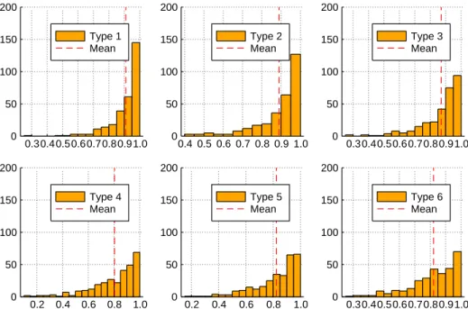
The results are shown in figures 3.2 and 3.3. Since these are HoC landscapes, as expected, F

is very close to one for all the types, however the mean becomes smaller as we go from type 1 to type 6, indicating that type 6 land- scapes have relatively greater additive contribution than type 1 landscapes.

A more interesting trend is observed for F

distributions. For types 1-3, the distribution is peaked close to 1, while for types 4-6 the peak shifts to a value close to zero. This indicates that types 1-3 show greater higher order epistasis than types 4-6. In [26], it was indicated that type 1 is likely to either show very high or very low higher order epistasis, however on average its F

is still larger than all the other types. In fact, the mean contribution to higher order epistasis reduces as we go from type 1 to type 6. The decline is strik- ingly similar to what is observed for F

, but the magnitude of the decline is much greater for F

. Not too surprisingly, this trend is also correlated with the trend seen for the mean number of peaks in the previous section (figure 3.1). Further, the minimum number of peaks, total sign epistasis and higher order epistasis, on average, consistently occur at type 4.

To summarize, the comparison with the Walsh spectra furthers our intu- ition about what kind of landscapes are encompassed by each of the 6 types.

3.4 Shapes in comparison to the _γ measure

The γ measure measures the correlation of mutational effects on different

backgrounds. As mentioned before, γ = Cor(s(g),s(g

)). Since it is a correlation,

Figure 3.4: The mean of the γ measure for landscapes of each of the six types.

-1.0 -0.5 0.0 0.5 1.0 0

20 40 60 80 100

Type 1 Mean

-1.0 -0.5 0.0 0.5 1.0 0

20 40 60 80 100

Type 2 Mean

-1.0 -0.5 0.0 0.5 1.0 0

20 40 60 80 100

Type 3 Mean

-1.0 -0.5 0.0 0.5 1.0 0

20 40 60 80 100

Type 4 Mean

-1.0 -0.5 0.0 0.5 1.0 0

20 40 60 80 100

Type 5 Mean

-1.0 -0.5 0.0 0.5 1.0 0

20 40 60 80 100

Type 6 Mean

Figure 3.5: The distribution of the γ measure for landscapes of each of the six types.

− 1 ≤ γ ≤ 1. Consequently, landscapes with magnitude epistasis have 0 ≤ γ < 1, landscapes with simple sign epistasis have − 1/3 ≤ γ < 1 and landscapes with reciprocal sign epistasis have − 1 ≤ γ < 0.

The results for landscapes belonging to different types are shown in figures

3.4 and 3.5.

For landscapes generated by the NK model, E[ γ ] ' 1 −

[25]. Now for HoC landscapes, K = L − 1 ⇒ E[ γ ] ' 0. For additive landscapes, γ = 1. Finally, for landscapes with maximal number of peaks

, γ = −1. So in some sense, γ and F

measure opposite effects. This explains why the plots of their means versus types (figures 3.3 (top) and 3.4) look like mirror images. Moreover, the results shown in figure 3.5 basically reinforce the fact that landscapes of type 6 are on average more correlated than those of type 1. The mean of γ is negative for types 1 and 2. This indicates the presence of sign and reciprocal sign epistasis motifs and agrees with what was seen in the section on fitness graphs. Moreover, for types 4-6, γ does not exceed 0.3. This indicates the departure from additivity due to magnitude epistasis.

1These are called egg-box landscapes

Application to empirical landscapes

4.1 Previous work

In an accompanying paper [36], Beerenwinkel et al exhibited the utility of their shape theory in analysing empirical data. They analysed pre-existing data of Elena and Lenski and showed that the new theory gave more insights into gene interactions in the fitness landscape than were previously known.

(a) The distribution of standard and non-standard tests

(b) The correlation of epistasis and the effect size of the muta- tions

Figure 4.1: Main results of [36]

They looked at a partial 9 locus landscape with 9 single mutants (all dele-

terious) and a restricted set of only 27 double mutants. Triple or higher mu-