Advanced data analysis for traction force microscopy and data-driven discovery of physical equations

(1)

Advanced data analysis for traction force microscopy and data-driven discovery of

physical equations

Inaugural-Dissertation

zur

Erlangung des Doktorgrades

der Mathematisch-Naturwissenschaftlichen Fakultät der Universität zu Köln

vorgelegt von

Yunfei Huang

aus Jingde, China

(2)

Berichterstatter: Prof. Dr. Gerhard Gompper (Gutachter) Prof. Dr. Dirk Witthaut

Prof. Dr. Benedikt Sabass

Tag der mündlichen Prüfung: der 30. November 2020

(3)

iii

“All things are numbers.”

Pythagoras of Samos

(4)

(5)

v

Abstract

The plummeting cost of collecting and storing data and the increasingly available computational power in the last decade have led to the emergence of new data analysis approaches in various scientific fields. Fre- quently, the new statistical methodology is employed for analyzing data involving incomplete or unknown information. In this thesis, new statistical approaches are developed for improving the accuracy of traction force microscopy (TFM) and data-driven discovery of physical equations.

TFM is a versatile method for the reconstruction of a spatial image of the traction forces exerted by cells on elastic gel substrates. The traction force field is calculated from a linear mechanical model connecting the measured substrate displacements with the sought-for cell-generated stresses in real or Fourier space, which is an inverse and ill-posed problem. This inverse problem is commonly solved making use of regularization methods. Here, we systematically test the performance of new regularization methods and Bayesian inference for quantifying the parameter uncertainty in TFM. We compare two classical schemes, L1- and L2-regularization with three previously untested schemes, namely Elastic Net regularization, Proximal Gra- dient Lasso, and Proximal Gradient Elastic Net. We find that Elastic Net regularization, which combines L1 and L2 regularization, outperforms all other methods with regard to accuracy of traction reconstruction.

Next, we develop two methods, Bayesian L2 regularization and Advanced Bayesian L2 regularization, for automatic, optimal L2 regularization. We further combine the Bayesian L2 regularization with the computational speed of Fast Fourier Transform algorithms to develop a fully automated method for noise reduction and robust, standardized traction-force reconstruction that we call Bayesian Fourier transform traction cytometry (BFTTC). This method is made freely available as a software package with graphical user-interface for intuitive usage. Using synthetic data and experimental data, we show that these Bayesian methods enable robust reconstruction of traction without requiring a difficult selection of regularization parameters specifically for each data set.

Next, we employ our methodology developed for the solution of inverse problems for automated, data- driven discovery of ordinary differential equations (ODEs), partial differential equations (PDEs), and stochastic differential equations (SDEs). To find the equations governing a measured time-dependent process, we construct dictionaries of non-linear candidate equations. These candidate equations are evaluated using the measured data. With this approach, one can construct a likelihood function for the candidate equations.

Optimization yields a linear, inverse problem which is to be solved under a sparsity constraint. We combine Bayesian compressive sensing using Laplace priors with automated thresholding to develop a new approach, namely automatic threshold sparse Bayesian learning (ATSBL). ATSBL is a robust method to identify ODEs, PDEs, and SDEs involving Gaussian noise, which is also referred to as type I noise. We extensively test the method with synthetic datasets describing physical processes. For SDEs, we combine data-driven inference using ATSBL with a novel entropy-based heuristic for discarding data points with high uncertainty. Finally, we develop an automatic iterative sampling optimization technique akin to Um- brella sampling. Therewith, we demonstrate that data-driven inference of SDEs can be substantially improved through feedback during the inference process if the stochastic process under investigation can be manipulated either experimentally or in simulations.

(6)

(7)

Kurzzusammenfassung

In vielen Bereichen der Naturwissenschaften haben die in den letzten Jahrzehnten stark sinkenden Kosten für Rechenleistung, sowie für die Speicherung großer Datenmengen, zur Herausbildung neuer Methoden der Datenanalyse geführt. Eine häufige Anwendung solcher Methoden besteht aus der Analyse und In- terpretation von Datensätzen die unvollständige Informationen enthalten. In dieser Doktorarbeit werden statistische Methoden entwickelt um einerseits die Genauigkeit der Zugkraftmikroskopie (ZKM) zu verbessern und andererseits auch eine datenbasierte Identifizierung von Gleichungen zur Beschreibung physikalischer Systeme zu verbessern.

Die ZKM ist eine vielseitig anwendbare Methode um die räumliche Verteilung von Zugkräften zu rekonstru- ieren, die von Zellen auf elastischen Gelsubstraten ausgeübt werden. Das Zugkraftfeld wird mit Hilfe eines linearen mechanischen Models berechnet, welches gemessene Substratverschiebung mit der gesuchten, zellgenerierten Spannung im Real- oder Fourierraum verbindet. Dies ist in der Regel ein schlecht kon- ditioniertes, inverses mathematisches Problem. Für gewöhnlich wird das Problem mit Hilfe von Regular- isierungsmethoden gelöst. In dieser Arbeit werden zunächst unterschiedliche Regularisierungsmethoden systematisch miteinander verglichen. Wir vergleichen zwei klassische Schemata, die L1- und L2 Regular- isierung, mit drei bislang ungetesteten Schemata und zwar mit dem Elastic Net, dem Proximal-Gradient Lasso und dem Proximal-Gradient Elastic Net. Es wird festgestellt, dass die Elastic Net Regularisierung, welche L1 und L2 Regularisierung kombiniert, alle anderen Methoden im Bezug auf die Genauigkeit der Zugkraftrekonstruktion übertrifft. Als Nächstes entwickeln wir zwei Methoden für eine automatisierte, optimale Regularisierung, die wir Bayessche L2 Regularisierungen nennen. Mit Hilfe synthetischer und experimenteller Daten zeigen wir, dass die Bayessche Methode eine robuste Rekonstruierung der Zugkraft ermöglicht ohne eine Wahl der Regularisierungsparameter speziell für jeden Datensatz zu erfordern. Als weitere Verbesserung der Bayesschen L2 Regularisierung führen wir eine schnelle Berechnung der nötigen Größen im Fourier Raum ein. Das Ergebnis ist eine vollständig automatisierte Methode zur Rauschreduk- tion welche robuste sowie standardisierte Zugkraftrekonstruktion erlaubt. Diese Methode wird als Soft- warepaket mit einer grafischen Benutzeroberfläche frei zugänglich gemacht.

Algorithmen zur Lösung inverser Probleme, wie sie für die ZKM wichtig sind, finden auch in vielen anderen Bereichen Anwendung. In den letzten Jahren insbesondere für das so genannte maschinelle Lernen.

Basierend auf zuvor für ZKM erprobten Regularisationsmethoden werden in dieser Arbeit verschiedene Ansätze für die datenbasierte Inferenz gewöhnlicher Differentialgleichungen (GDGLs), partieller Differ- entialgleichungen (PDGLs), und stochastischen Differentialgleichungen (SDGLs) erprobt. Um die bestim- mende Gleichung für einen gemessenen, zeitabhängigen Prozess zu finden, werden Bibliotheken verschiede- ner Gleichungskandidaten angelegt. Die Optimierung der Wahrscheinlichkeitsfunktion für die verschiede- nen Gleichungskandidaten verlangt die Lösung ein linearen, inversen Systems. Hierfür wird eine Bayessche L1 Regularisierung mit einer iterativen Elimination überflüssiger Ergebniskomponenten kombiniert. Die entwickelte Methode mit dem Akronym ATSBL ist für die Inferenz von GDGLs, PDGLs und SDGLs ver- wendbar. Ein umfangreicher Test mit synthetischen Datensätzen zur Beschreibung physikalischer Prozesse ist erfolgt. Für SDGLs kombinieren wir ATSBL mit einer neuen entropiebasierten Heuristik um Daten- punkte mit großer Messungenauigkeit zu eliminieren. Zu guter Letzt wird eine iterative Stichprobenop- timierung ähnlich dem Umbrella Sampling entwickelt, um sie mit ATSBL zu kombinieren. Anhand von Beispielen wird gezeigt, wie durch gezielte Störung eines gemessenen stochastischen Prozesses die dem Prozess zugrundeliegenden Differentialgleichungen genauer bestimmt werden können.

(8)

(9)

ix

Acknowledgements

First of all, I would like to express my gratitude toward Prof. Dr. Gerhard Gompper and Prof. Dr. Benedikt Sabass for providing me with this PhD position at the Theoretical Soft Matter and Biophysics institute (ICS-2/IAS-2) at Forschungszentrum Jülich three years ago and supervising me in the last more than three years for my PhD thesis. Thank you for introducing me to the fantastic world of advanced data analysis for the biophysical problems and something I had never thought possible when I was in the previous studies. Thank you for teaching me both intuition and rigor in the exploring and studying a new field. Thank you for sometimes subtly pushing me back towards thinking about the larger questions and the theoretical reasons when we solved a minor numerical or mathematical issue. Thank you for teaching me, both consciously and unconsciously, how good theoretical biophysics is done. Thank you for carefully teaching and instructing me how to conceive and write a fantastic scientific article. Thank you also for providing me many opportunities to learn broadly and to participate the biophysical conferences and schools. It is your excellent ideas and encouragement that have enable me to do this work presented in this thesis. I will keep fond memories of these three years in Jülich learning from you and working with you and hope that our paths will cross again many times in near the future.

I also would like to express my gratitude to Prof. Dr. Dirk Witthaut for accepting to review my doctoral thesis and to Prof. Dr. Markus Braden for accepting to act as the chair for my doctoral thesis defense committee.

I want to thank Prof. Dr. Rudolf Merkel, Dr. Christoph Schell, Prof. Dr. Tobias B. Huber, and Nils Hersch for the good collaboration on the project of traction force microscopy and providing the experimental test data. I am also grateful to our collaborators Prof. Dr. S.

V. Plotnikov (University of Toronto) and C. Schell (AlbertLudwigs-University Freiburg) in the study of a Bayesian traction force microscopy method with automated denoising in a user-friendly software package for providing the experimental test data.

I thank all my colleagues at the Forschungszentrum Jülich not only for your direct helps in the physics, mathematics, and computer techniques, but also for your enthusiasm for discussing wide-ranging topics in science and beyond to shape and develop my own thinking more like a scientist. It is the precious moments we shared during and outside of work. I then want to thank all members of our group Ahmet Nihat ¸Sim¸sek, Andrea Bräutigam, and Kai Zhou for discussing the project and together through the good times and the difficult times.

A special thank you goes to my supervisors, my wife, Carlos Plúa, Andrea Bräutigam, Chao- jie Mo, Kai Zhou, and Ahmet Nihat ¸Sim¸sek for correcting this manuscript and showing great patience with my English. I also would like to thank Christian Philipps and Joscha Mecke for helping the translation of this German abstract.

Finally, I want to express my deep gratitude towards all members of my family and all close friends who even if sometimes from afar have always been with me for their too many encouragement and support during these years.

Yunfei Huang Forschungszentrum Jülich August 2020

(10)

(11)

xi

List of Figures

1.1 Schematic overview of Non-Bayesian and Bayesian methods for solving linear

inverse problems . . . 6

1.2 Structures of the cytoskeleton in cells . . . 8

1.3 Extracellular structures . . . 10

1.4 Mechanical models and imaging techniques . . . 11

1.5 Schematic different methods for measuring forces on a single cell . . . 13

1.6 Two methods for measuring forces of cell-ECM connections . . . 14

1.7 Several results of traction forces obtained by using TFM . . . 16

1.8 Schematic diagram of the procedure for performing high-resolution traction force microscopy . . . 17

1.9 Identification of ordinary and partial differential equations by using sparse symbolic regression . . . 20

1.10 The neural network algorithm for the identification of partial differential equations from type II noisy data . . . 21

1.11 The identification of stochastic differential equations . . . 22

2.1 Well posedness is defined by the relationships between elements, spaces, the operator, and metrics . . . 26

2.2 The 2D contour and exact solutions for different regularization methods . . . 29

2.3 Three different approaches to select the L2 regularization parameter . . . 31

2.4 Graphical model of the sparse Bayesian approaches . . . 42

3.1 Schematic representation of a typical traction force microscopy (TFM) setup and different reconstruction methods for TFM . . . 47

3.2 Analytically calculated displacement field around 15 circular traction patches 50 3.3 Classical methods for selecting the regularization parameter . . . 54

3.4 Systematic tests illustrate substantial ambiguity in the choice of regularization parameters . . . 55

3.5 Results of L1 regularization using CVX for differentλ1for Fig. 3 of the main text . . . 56

3.6 The elastic net (EN) outperforms other reconstruction methods in the presence of noise and when applied to undersampled data . . . 57

3.7 Results of L1 regularization using CVX and IRLS for differentλ₁for Fig. 3 of the main text . . . 58

3.8 Bayesian L2 regularization (BL2) and Advanced Bayesian L2 regularization (ABL2) are robust methods for automatic, optimal regularization . . . 59

3.9 The determination of regularization parameters from different methods for the experimental data . . . 60

(16)

3.10 Test of all reconstruction methods using experimental data. (a) Image of an adherent podocyte with substrate displacements shown as green vectors . . . 61 3.11 L-curve selection regularization parameter for the data for analysis of traction

time sequences . . . 62 3.12 Bayesian L2 regularization robustly adapts to different traction levels allow-

ing quantitative analysis of time series . . . 63 4.1 Schematic of traction force microscopy (TFM) to measure cellular traction on

flat elastic substrates . . . 69 4.2 Graphical user interface of the provided software for regularized FTTC and

BFTTC . . . 73 4.3 The software provides two methods to calculate cellular traction forces from

experimental data . . . 74 4.4 Validation of the Bayesian method for regularization parameter choice . . . . 76 4.5 Reconstruction quality of BFTTC compared to other regularization methods . 77 4.6 Test of Bayesian Fourier transform traction cytometry (BFTTC) using experi-

mental data . . . 79 5.1 Exemplary results for data-driven identification of the ordinary differential

equations for the Lorenz system . . . 88 5.2 The identification of partial differential equations for Burgers’ equation . . . . 89 5.3 Testing the identification of partial differential equations with the KdV equation 90 5.4 The identification of partial differential equations for Navier-Stokes equations 91 5.5 The identification of partial differential equations for reaction-diffusion equa-

tions . . . 92 5.6 The neural network deep learning reduces the type II Gaussian noise data and

the governing equations is identified by using ATSBL . . . 94 5.7 The neural network deep learning method improves the identification of the

Kuramoto-Sivashinsky (KS) equation . . . 94 5.8 The identification of stochastic differential equations for a double-well poten-

tial with an inhomogeneous diffusion . . . 96 5.9 An improved identification of stochastic differential equations through using

a probability threshold . . . 97 5.10 The identification of stochastic differential equations is improved by using

sampling strategy . . . 98 5.11 The identified SDEs from three-well potential by using an automatic iterative

sampling optimization . . . 101 5.12 The identified SDEs from four-well potential by using an automatic iterative

sampling optimization . . . 103 5.13 The identification of two-dimensional stochastic differential equations . . . . 105 B.1 Analytical displacement fields around one circular traction patch . . . 114 B.2 Additional error quantification for the regularization methods in Fig. 2 of the

main text . . . 114 B.3 Parameter-dependence of EN regularization error for Fig. 2 of the main text . 115 B.4 Parameter-dependence of PGEN regularization error for Fig. 2 of the main text 115 B.5 L-curves for the regularization methods shown in Fig. 2 of the main text . . . 115

(17)

xvii B.6 Exemplary traction fields reconstructed from noise-free artificial data . . . 116 B.7 Exemplary traction fields reconstructed with Bayesian methods from artificial

data with 5% noise . . . 117 B.8 Exemplary comparison of error measures with artificial data using ten differ-

ent methods . . . 117 B.9 Comparison of various Bayesian methods using the real data from Fig. 5 of

the main text . . . 118

(18)

(19)

xix

List of Tables

3.1 Overview of the runtime RAM requirement for each method . . . 57 4.1 Computation time for different methods . . . 78

(20)

(21)

xxi

List of Abbreviations

ECM Extracellular Matrix TFM Traction Force Microscopy STED Stimulated Emission Depletion BEM Boundary Element Method

DTMA Deviation of Traction Magnitude at Adhesions DTMB Deviation of Traction Magnitude in the Background SNR Signal to Noise Ratio

DMA Deviation of the traction Maximum at Adhesions L2 L2 Regularization

L1 L1 Regularization

EN Elastic Net Regularization PGL Proximal Gradient Lasso PGEN Proximal Gradient Elastic Net BL2 Bayesian L2 Regularization

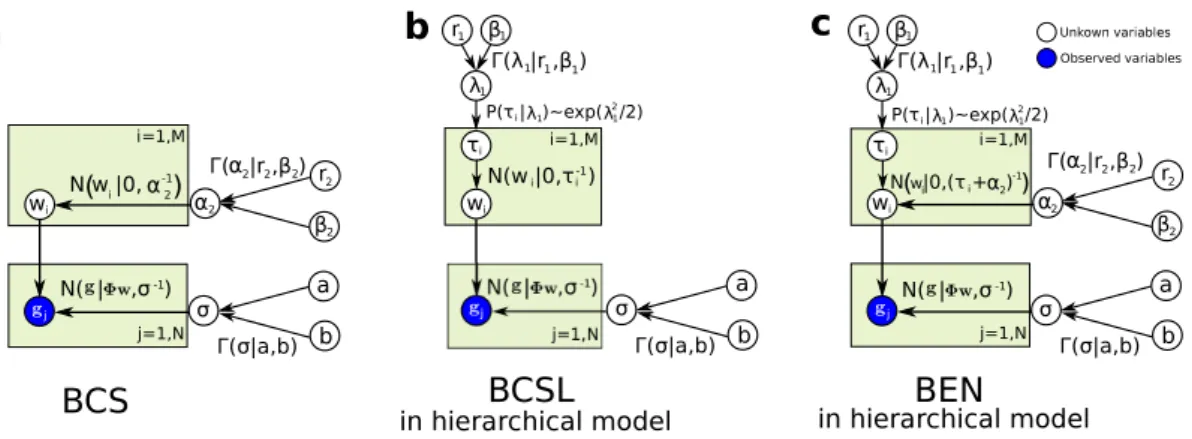
ABL2 Advanced Bayesian L2 Regularization BCS Bayesian Compression Sensing

BCSL Bayesian Compression Sensing using Laplace prior BL Bayesian Lasso

BEN Bayesian Elastic Net

IRLS Iterative Reweighed Least Squares FTTC Fourier Transform Traction Cytometry

BFTTC Bayesian Fourier Transform Traction Cytometry MLE Maximum Likelihood Estimation

MAP Maximum a Posteriori GCV Generalized Cross Validation MCMC Markov chain Monte Carlo ODE Ordinary Differential Equations PDE Partial Differential Equations SDE Stochastic Differential Equations SVD Singular Value Decomposition RVM Relevance Vector Machine

ATSBL Automatic Threshold Sparse Bayesian Learning UP Universal Prediction

AISO Automatic Iterative Sampling Optimization

(22)

(23)

xxiii

List of Symbols

I Self-information or Information content

X_i State

H Total uncertainty or Entropy

g Observed vector

N Size ofg

Φ Observed matrix

w Unknown vector

M Size ofw

s Noise vector

wˆ Reconstructed vector

I Unit matrix

λ₁ L1 regularization parameter λ2 L2 regularization parameter

f_GCV Generalized cross-validation (GCV) function f_QOC Quasi-optimality criterion function

W Unitary wavelet transform W^∗ Inverse wavelet transform G Observable random variable forg W Non-observable random variable forw

S Random variable fors

p(w) Prior

Z_w Normalization of prior p(g|w) Likelihood

Z_g Normalization of likelihood 1/α Variance of prior

1/β Variance of likelihood p(w|g, α, β) Posterior

Z_K Normalization of posterior p(g|α, β) Evidence or Marginal likelihood µµµ Mean of posterior

Σ Covariance of posterior

w_MP Maximum posterior

A Hessian

C Covariance of evidence

L Logarithm of evidence

U_i(x) Continuous displacement field Fj(x⁰) Continuous force field

x= (x₁, x₂) Two-dimensional vector

(24)

Ω Whole surface of the substrate

E Young’s modulus

ν Poisson’s ratio

Gij Green’s function in real space δ_ij Kronecker delta function z Vertical position of the substrate u_i Discrete displacement field fj Discrete traction force field

h Shape function

M Coefficient matrix betweenuiandfj

k= (k1, k2) Wave vector

G˜_ij Green’s function in Fourier space t^real Real traction

t^recon Reconstructed traction

α,ˆ βˆ Optimal parameter

λˆ Optimal regularization parameter

t Time

z,u Measurement data

˙

z Time derivative of measurement data ux,uxx,· · · Space derivative of measurement data

Θ Augmented library

z^P² Higher polynomials

g Drift function

h Diffusion function

L(x, t)ˆ Fokker-Plank operator

D⁽ⁿ⁾ Kramers-Moyal (KM) coefficients U(x, t) Potential energy function

Q Number of bins

∆t Time step

LEN Elastic net regularization L_{M SE} Mean squared error

LReg Regression based cost function

u_recon Reconstructed dataset

T Probability threshold

(25)

xxv

To my family. . .

(26)

(27)

1

Chapter 1 Introduction

1.1 Historical development of data analysis methods

More than 60 years ago, John Tukey [1] envisioned a future of science that is focused on learning from data, or “data analysis”, which is a process of using statistical practices to describe, represent, organize, evaluate, and interpret data. Nowadays, there exists a large number of automated techniques for generating, collecting, and storing trillions of measurement data points every day in the whole world. For this reason, data analysis has become increasingly important in various scientific and engineering fields.

To introduce the concept of statistical learning, we start by considering the classical regression problem which aims at estimating the relationship between a given data set consisting of a N-dimensional vector of input datag(often called observed data) with given parameters in aN ×M matrixΦand a M-dimensional vector of dependent dataw(often called the output- or unobserved data). The most common form of regression analysis islinear regression[2,3], in which the model is written in matrix notation as

g=f(w) =Φw+s, (1.1)

wheresis an observed or unobserved error variable, often called noise. In more general cases where the relation betweenwandgmay be a non-linear functionf(w)mapping the inputs to the outputs can also be defined [4–6]. In mathematical physics, the formulation of theforward problemfor a physical field involves [7]: (1) The domain in which the field is studied. (2) The equation function that describes the field. (3) The initial conditions. (4) The conditions on the boundary of the domain. The inverse problem consists of finding functions used for the forward problem, for example, the unknownf(w)in Eq. (1.1). Given g andΦ, the calculation ofw is referred to as solving aninverse problem. This inverse problem is historically a long-standing issue and various approaches have been invented and developed to deal with this problem in past hundreds of years. Theleast-squares method[8]

was a common early approach for solving an inverse problem like the one associated with Eq. (1.1).

1.1.1 Classic approaches for solving inverse problems

Least-squares method Over 200 years ago, the method of least squares was first published by Adrien-Marie Legendre in 1805 [9,10]. It is usually also credited to Carl Friedrich Gauss [11] because in 1809 Carl Friedrich Gauss [12] published the method of calculating

(28)

the orbits of celestial bodies by using the least-squares method and he claimed to have been in possession of the method since 1795. The simple least-squares fit minimizes the sum of the squares of the difference between the observed datagiand the fitting function evaluated atw_i: PN

i=1(g_i −f(w_j))². If each standard deviationσ_i for the observed data g_i is given, the least-squares method can also be written as the minimization ofPN

i=1((gi−f(wj))/σi)², which is called aχ²fit. Thisχ² fit was first described by the German statistician Friedrich Robert Helmert in 1876 [13,14] and was independently rediscovered by the English mathematician Karl Pearson in 1900 [15]. The main disadvantages of this simple least-squares method are the requirement of small deviations between data and model, which allows one to assume a Gaussian distribution and causes sensitivity to outliers.

In 1809 [12], Gauss extended the least-squares method through a probabilistic perspective.

He combined the Lambert-Bernoulli idea [16,17] with Laplace’s analytical formulation of inverse probability [18,19]. Requiring that the mode of what is nowadays called the posterior probability distribution equals the arithmetic mean, Gauss derived the normal distribution [12,20]. From the least-squares method to modern methods for solving complex inverse problems, normally distributed errors appear in many statistical approaches.

Maximum likelihood estimation Before 1912, maximum likelihood estimation (MLE) oc- curred in rudimentary forms, but not under this name. Some of the estimates called “most probable” would today have been called “most likely” [20]. In 20th century statistics, the making of maximum likelihood was one of the most important developments [21,22]. In 1912, the British statistician and geneticist R. A. Fisher [23] started producing one of the earliest contribution to modern statistics by using a simple maximum likelihood method (“absolute criterion”) to estimate unknown parameters. R. A. Fisher introduced the term

“likelihood” in 1921 [24] and the name “maximum likelihood estimate” finally appeared in the article “On the mathematical foundations of theoretical statistics” in 1922 [25]. Let w be an unobserved data set andgbe a set of observed data. The conditional probability ofg, givenw,p(g|w) is calledlikelihood. MLE is to maximize the likelihood function L(w)with respect to the unobserved data w. For example, consider the maximum likelihood estimation applied for the inverse problem in Eq. (1.1) [26]. The errorssare assumed to be values of a random variableSwhich follows a Gaussian distributionS ∼ N(0,1/β), where the variance is1/β. Thus, the likelihood is written asp(g|w) = (2π/β)^−N/2exp − β(g−Φw)²/2

. To obtainw, one maximizes the log-likelihood function which is denoted asl(w) =−N/2 log(2π) +N/2 logβ−β/2 (g−Φw)^T(g−Φw)

. Here, the maximum likelihood estimation is equivalent to the east-squares method for minimizingPN

i=1(gi−Φijwj)². Between 1912 and 1922, R. A. Fisher had produced three justifications and three names for the technique of MLE [20,22]. Although R. A. Fisher is certainly the father of maximum likelihood analysis, his attempts to prove the procedure remained largely fruitless [27]. The solid theoretical basis for the maximum likelihood estimation procedure was laid by Samuel S. Wilks in 1938 [27], now also called Wilks’ theorem. This theorem states that the error in the logarithm of likelihood values for estimates from multiple independent observations is asymptoticallyχ²-distributed, which enables convenient determination of a confidence region around any estimate of the parameters.

Bayesian methodology The foundations of Bayesian probability theory were posthumously published in Thomas Bayes’ article “An Essay Towards Solving a Problem in the Doctrine of Chances ” in 1764 [28]. Later, the french mathematician, Pierre Simon Laplace independently

(29)

1.1. Historical development of data analysis methods 3 rediscovered the Bayes’ modern mathematical form in the article “Mémoire sur la probabil- ité des causes par les événements” in 1774 [18] and the later article “Théorie analytique des probabilités” in 1812 [29]. Like in MLE,wis an unobserved data set andgis an observed data set. The conditional probabilityp(w|g)expresses the probability of finding the sought-for quantitiesw, given the observed quantitiesg. Theposteriorprobability distributionp(w|g) is typically not known. Frequently, however, the reverse conditional probability distribution p(g|w)is known either based on generic assumptions regarding the experimental system or because one is dealing with numerical simulations. The posterior probability and the likelihood can be related to each other by making use of the unconditional probabilitiesp(g)and p(w). The standard modern-days Bayes’ rule was first given by Laplace as [30]

p(w|g) = p(w,g)

p(g) = p(g|w)p(w)

p(g) ∝p(g|w)p(w). (1.2)

Here, p(w,g)is the joint probability distribution. Since p(w) can reflect a prior information about the sought-for quantityw, it is called "prior". In contrast, p(g)is the unconditional probability distribution for observing the valuesgand is therefore called "evidence" or

"marginal likelihood". In Eq. (1.2), the posterior distribution is proportional to likelihood multiplied by prior. Themaximum a posterior(MAP) estimate ofwis defined as that value that maximizes the likelihood multiplied by a prior. Thus, MLE is a special case of the MAP estimation, where a uniform priorp(w) =const. is assumed in Eq. (1.2). However, the Bayesian methodology provides much broader flexibility since one can choose priorsp(w)together with the likelihood function.

1.1.2 Challenges and modern approaches for solving inverse and ill-posed problems

We have introduced the classic approaches to solve the inverse problem in Eq. (1.1). One common challenge is that the inverse problem is often a so-calledill-posed problem. The study of inverse and ill-posed problems began in the early 20th century [7]. In 1902, J. Hadamard proposed the concept of well-posedness of problems for differential equations [31] and he termed a problem well-posed if there exists a unique, robust solution to this problem. He also gave an example of an ill-posed problem, namely, the Cauchy problem for the Laplace equation, where the solution does not depend continuously on the data and any small change in the data causes large changes to the solution [32–34]. The challenge of solving ill-posed problems occurs in almost all fields of science, particular examples are image reconstruction [35,36], traction force reconstruction [37,38], machine learning [39,40], seismic exploration [41], tomography [42], astronomy [43], and air and water quality control [44].

One common important property of ill-posed linear problems is the strong sensitivity of the solutions to small perturbations in the equation parameters. In linear regression Eq. (1.1), the well-posedness of the solution depends on the matrixΦand it can be analyzed by using a perturbation approach [7,45]. Introducing the perturbationsδgandδw, Eq. (1.1) becomes g+δg=Φ(w+δw). We can also writeδg=Φδw, which impliesδw=Φ⁻¹δgandkδwk2≤ kΦ⁻¹k2kδgk2. The unperturbed Eq. (1.1) yieldskgk2≤ kΦk2kwk2. Thus, the estimate for the relative error of the solution becomeskδwk₂/kwk₂≤ kΦk₂kΦ⁻¹k₂kδgk₂/kgk₂, which shows

(30)

that the error is determined by the constant

κ(Φ) =kΦk₂kΦ⁻¹k₂, (1.3)

whereκ(Φ)is called thecondition numberof a system. A system with alargecondition number is said to be ill-posed because small variations in the inputδgmay lead to relatively large variations in the solution. Variations (errors) of input data always exist in measure- ments or simulations. Solving ill-posed problems involving such input data is challenging with classical approaches, such as those from least-squares methodology. However, inverse and ill-posed problems can often be solved by imposing an additional regularization constraint when performing a least-squares optimization. A general form of this regularization procecdure when extending the linear regression Eq. (1.1) is written as

ˆ

w=argmin

w

(g−Φw)²+λH(w)

, (1.4)

wherewˆ is the solution of inverse and ill-posed problem andλH(w)represents the regularization constraint with an unknown parameterλ >0. Various regularization approaches have been developed in the past 80 years.

1.1.2.1 Regularization approaches

In 1943 [46], A. N. Tikhonov pointed out the practical importance of ill-posed problems and the possibility of finding stable solutions to them. The nowadays standard approach to solve ill-posed problems is called ridge regression and was published by David L. Phillips [47] in 1962 and A. N. Tikhonov in 1977 [32]. The ridge regression or Tikhonov regularization relies on the constraintλH = λ2kwk²₂involving the 2-norm and therefore it also called L2 regularization. The solutions of L2 regularization are typically smooth and non-sparse and the computation is efficient because analytical expressions can be derived for the L2 regularization.

In 1986, geophysicists observed that the constraintλH=λ1kwk1can be successfully applied to compute a sparse reflection function indicating changes between subsurface layers [48].

In 1996, Robert Tibshirani [49] greatly popularized the use of L1-norm and related greedy methods in statistics, called the Lasso, or Lasso regression, or L1 regularization. The main property of L1 regularization is the sparsity of solutions, which means that the solution contains only few non-zero components.

In 1994, the method of L0-norm constraintλH = λ0kwk0 was suggested by D. P. Foster and E. I. George [50] and today this regularization method is called L0 regularization or best subset selection [51]. The solutions from L0 regularization are for certain sparse models more accurate than the solutions obtained from L1 regularization [52]. However, computational challenges related to L0 regularization result from the discontinuity and nonconvexity of the L0-penalty function. This issue is usually dealt with by replacing the L0-penalty function with a continuous or convex approximation function [53,54].

In 2005, Zou and Hastie [55] introduced the elastic net regularization which combines the L2- with the L1-norm constraintλH =λ₂kwk²₂+λ₁kwk1. This approach balances smooth- ness and sparsity of the solutions from ridge- and Lasso regression, respectively. Recently, the elastic net regularization is widely employed in various scientific applications such as

(31)

1.1. Historical development of data analysis methods 5 studying anticancer drug sensitivity [56,57], gene expression [58], structure and function of ocean microbiome [59], and face recognition [60].

Here, we have briefly introduced five regularization approaches to deal with inverse and ill-posed problems. When one uses these approaches, the challenge is to identify the optimal regularization parameterλ, which is a priori unknown. A number of methods exist for selecting the regularization parameters, such as the L-curve [61], generalized cross- validation [62] or quasi-optimality criterion [63]. However, these methods mostly rely on heuristics and manual selection of the regularization parameter is usually necessary. Those problems can be overcome by using Bayesian analysis.

1.1.2.2 Bayesian regularization approaches

The heuristic regularization approaches discussed above can be related to the concept of maximizing the posterior probability in a Bayesian framework. To illustrate this connection, we assume, as for the maximum likelihood estimator of the linear regression Eq. (1.1), a noisesthat obeys a Gaussian distributionsi ∼ N(0,1/β). Here, the prior is also assumed to be a Gaussianw_i ∼ N(0,1/α), where the variance is1/α. According to Bayes’ rule in Eq. (1.2), the posterior distribution is written asp(w|g) = (2π/β)^−N/2(2π/α)^−M/2exp − β(g−Φw)²/2

exp −αw²/2

∝exp −β(g−Φw)²/2−αw²/2

. To obtainw, we maximize the posteriorwˆ =argmax

w

[−β(g−Φw)²/2−αw²/2], where the form is the same as the L2 regularizationwˆ =argmin

w

[(g−Φw)²+λ2w²]with λ2 = α/β. The constraintλH in each of the regularization approaches that were mentioned above can be related to a particular prior function, for example, here, L2 regularization yields a Gaussian prior. It is not difficult to find that the L1-, L0-, and elastic net regularization respectively, are equivalent to a MAP estimation employing a Laplace priorp(w)∝exp(−λ1kwk1)[64], L0-regularized priorp(w)∝exp(−λ0kwk0)[65], and Elastic net priorp(w)∝exp(−λ1kwk1−λ₁kwk²₂)[66].

While these results connect the regularization approaches to the Bayesian MAP estimates, the challenge of selection of regularization parameter remains when using only the MAP approach. However, this challenge can be overcome in the Bayesian framework.

Bayesian regularization Bayesian regularization[67,68] involves two levels of inference:

(1) Choose models and fit data (model fitting). (2) Rank the alternative models (model comparison). In the first level of inference, the particular model is assumed and fitted to the data, which can be done with a MAP estimation procedure. In the second level of inference, the evidence for the model parameters is calculated, for example, by using the marginal likelihood which is given in the Bayes’ rule of Eq. (1.2). This process embodies the colloquial “Occam’s razor”, which ensures that overly complex models will not be preferred over simpler models unless the data supports them. The details of Bayesian regularization employing a Gaussian prior will be laid out in Chapter2.

Sparse Bayesian learning In 2001, M. E. Tipping [69] demonstrated a probabilistic Bayesian learning framework where the solution is assumed to consist of only few basis functions, which is therefore called relevance vector machine (RVM). This work is an extension of Bayesian regularization techniques because it also utilizes the maximum evidence principle estimate the parameters or hyperparameters of likelihood and prior. In 2003, M. E.

Tipping and A. C. Faul [70] described a highly accelerated algorithm which exploited the

(32)

evidence function [67] to enable maximization via a principled and efficient sequential ad- dition and deletion of candidate basis functions. The details of this approach will be laid out in Chapter2. Sparse Bayesian learning approacheswere successfully applied to reduce the di- mensionality of sensor data. This technique is now called Bayesian compressive sensing [71, 72]. These Bayesian sparse learning approaches require Markov chain Monte Carlo (MCMC) methods [73–77] or a more efficient variational Bayesian (VB) analysis [67,78].

All the above approaches to solve inverse problems with an unknown vectorw, rely on the provision of a matrixΦ and a (measurement) data vector g. However, in some cases the matrixΦmay be unknown. For example, in classification tasks one may have a set of training data for the relationship between the classifierˆgand the feature vectorg, but the system matrixXand the noisebare unknown inˆg= k(g) = Xg+b. In such cases, one can use neural networks and methods from deep learning to obtain the unknown system parameters.

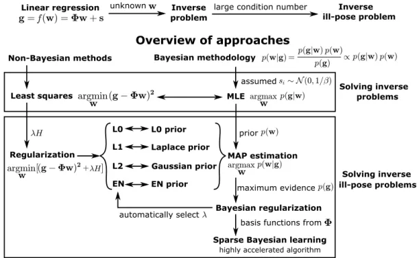
Overview of approaches

problem ill-pose problem

Linear regression unknown Inverse large condition number Inverse

Bayesian methodology

Least squares

Regularization

Non-Bayesian methods

L0 L1 L2 EN

MLE

MAP estimation

Bayesian regularization assumed

prior L0 prior

Laplace prior Gaussian prior

EN prior maximum evidence

Sparse Bayesian learning basis functions from

problems Solving inverse

ill-pose problems Solving inverse

automatically select

highly accelerated algorithm

Figure 1.1:Schematic overview of Non-Bayesian and Bayesian methods for solving linear inverse problems.

1.1.3 Deep learning for analysis of noisy data

Deep learningcan be traced back to 1943 [79], when W. S. McCulloch and W. H. Pitts created a computer model based on the neural network of the human brain. Recently, thousands of deep learning methods have been developed that involve, for example, backpropagation algorithm, convolutional neural networks, recurrent neural networks, recursive neural networks, autoencoders, and graph neural networks. Here, we utilize the example of noise reduction to explain the central idea of supervised neural networks [80,81]. Given an input vectort, e.g., a space or time vector, and a target noisy datag, we train a neural network with the given relation betweentandg. A successfully trained network will, for any givent, produce an outputˆgthat is close to the target vectorg. To demonstrate this concept, a two-layer neural network [80] is employed. The hidden layer is written asζ^X¹^,b¹(t) =ζ(X₁t+b₁), whereζ is an activation function, e.g., ζ(·) = tanh(·). X1 and b1 are respectively called

(33)

1.2. Background information on measurement of cellular forces 7 weights and biases. The output layer is written asˆg=ζ^X¹^,^b¹(t)X2+b2. These unknown weights and biasesX₁,b₁,X₂andb₂of each layer are learned by the minimization of a cost function, which is the sum of the deviation between the output and the target. Using such a neural network, the noise in the inferred outputˆgtypically can be significantly reduced [82].

In Figure1.1, we present an overview of methods for solving inverse problems. The Bayesian methodology has the advantage of allowing one to prescribe clearly defined assumptions in the form of priors which then automatically produce robust solutions. However, many approaches for solving inverse problems in physics and biophysics still exclusively rely on non-Bayesian methods. In this thesis, we systematically test the classic approaches and develop new methods to solve inverse ill-posed problems in two applications, namelytraction force microscopyanddata-driven discovery of physical equations. To prepare the stage, we will in the following sections introduce background information on these two applications.

1.2 Background information on measurement of cellular forces

The mechanical behaviour of cells and tissues plays a crucial role in a variety of biological, biophysical and biochemical processes, including cell migration [83,84], tissue morphogen- esis [85,86], wound healing [87,88], cell differentiation [89,90], and gene expression [91,92].

Many of the relevant mechanobiological processes occur on a subcellular lengthscale, for example at micrometer-sized cellular adhesions and at filopodia. However, mechanobiology also plays a critical role on the level of multiple cells and on lengthscales of millimeters, for example in embryonic development [93,94]. The mechanical behaviours of cells are not only controlled by biochemical reactions inside of cells, but also depend on the mechanical properties ofextracellular matrix(ECM). To understand the interplay of extracellular and intracellular mechanics and biological regulation, a reliable and accurate method for the measurement of cellular forces is required. Over the past 50 years, various approaches have been developed for this purpose. In Ref. [95], different kinds of methods were systematically summarized. Various approaches and tools for measuring the forces generated on ECM were also reviewed in Ref. [96].

In this section, some background information on the mechanobiology of cells is introduced.

First, we introduce the mechanical structures: the cytoskeleton, transmembrane, and extracellular structures. Then, we introduce different mechanical models for the structures.

Finally, we summarize several approaches and tools to measure the mechanical forces.

1.2.1 Mechanical structures of cell

1.2.1.1 Cytoskeleton

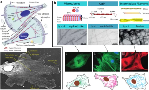
Thecytoskeleton(CSK) is a polymeric fiber-based scaffold for structural integrity inside cells.

These scaffolds not only serve as a traffic system for intracellular transport [97], for example, helping to ship vesicles or organelles, but also are important mechanical structures for cells migration. Usually, the CSK consists of at least three distinct filamentous elements: microtubules, actin-CSK, and intermediate filaments, illustrated in Fig.1.2(b). Here, we briefly introduce each of these structures and their mechanical properties.

• Microtubuleshave a length up to roughly50µmand are composed ofα- andβ-tubulin.

The outer diameter of a microtubule is about25 nm and the inner diameter is about

(34)

a b

Actin laments Myosin laments

iii ii

i

Figure 1.2:Structures of the cytoskeleton in cells. (a-Top) Illustration of the components of the actin cytoskeleton in representative fibroblast-like cells. The direction of migration is denoted by the wide gray arrows. (a-Bottom) Electron micrograph of the cytoskeleton of aXenopus laevisfibroblast. (b-Top) The cytoskeleton (CSK) has the three types of biopolymers: microtubules, actin and intermediate filaments. The three types of CSK pertain to different stiffness regimes because of their differing filament architectures.

(b-Middle) Fluorescence micrographs for each type of CSKs in real cells.

(b-Bottom) Schematic graphs show that each type of CSKs is how to distribute inside cells. (Figure (a) adapted from T. Svitkina 2018 [98]. Figure (b) adapted from F. Huber, 2011 [99] with source material from D. E. Ingber, 2003 [100] and J.

R. D. Soiné, 2014 [101].)

13 nm. They are very rigid polymer tubes that usually emerge as individual fibers, which are typically associated with organelle positioning and intracellular transport.

• Actin-CSKsare composed of monomeric G-actin and the linear polymeric F-actin with a diameter from4 nmto7 nm[102]. Actin filaments are semi-flexible polymers appear- ing as cross-linked networks within cells, illustrated in Fig.1.2(b-ii) [100]. The actin CSK is a dynamical structure that appears in different forms, including compact stress fibers and finely crosslinked nets.

• Intermediate filamentshave a diameter of roughly50 nm, which is between the size of actin filaments and microtubules, illustrated in Fig.1.2(b-iii) [100]. Intermediate filaments are composed of a family proteins including desmin, keratins, and lamins.

The CSK is the essential structure creating motility-driving forces. These forces are generated by polymerization and the interaction of the F-actin network with myosin motors.

The former, the polymerization of actin filaments at the leading edge of cells, can move the edge forward [103] and the force generation in this process can be explained by two models, ratchet models [104, 105] and autocatalytic models [106, 107]. The latter, the myosin motors move on actin filaments through a usual three-step process of binding, power-stroke, and unbinding [108], which generates contractile forces. The force generated from each of the motors is extremely tiny. For example, to lift a5 kgweight, about 10¹³myosin motors

(35)

1.2. Background information on measurement of cellular forces 9 are required [108]. These two motility-driving mechanisms not only result in motion and deformation of the cytoskeleton and the cell, but also produce a mechanical load on the extracellular structures.

1.2.1.2 Transmembrane and extracellular structures

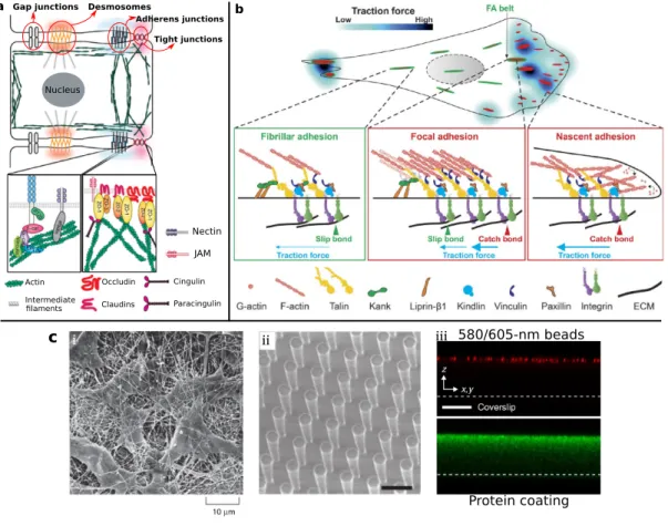
The mechanical connection between the intracellular CSK and the extracellular world is maintained by dedicated molecular structures. Figure1.3(a) shows a schematic diagram of different types of cell-cell adhesions, which include gap junctions, tight junctions, adherens junctions, and desmosomes [109]. These cell-cell adhesions not only can transfer mechanical forces from one cell to another cell, but also provide an aisle for different molecules between two cells, for example, ions and electrical impulses. Here, we briefly summarize the structures and their properties.

• Gap junctionare intercellular connections with a variety of transport functions and, for instance, allow the passage of small molecules or electrical signals.

• Tight junctions, also called occulding junctions, seal the space between neighboring cells and can control the passage of ions and small moclecules.

• Adherens junctionsprovide the strong mechanical attachments between cells. Adherens junctions can contain nectin-afadin or E-cadherin-a-catenin-vinculin bonds, illustrated in Fig.1.3(a) and they are linked to the actin-CSK inside the cell.

• Desmosomesare localized patches, which can hold two adjacent cells closely together [110].

Desmosomes are attached to intermediate filaments of keratin in the cytoplasm, illustrated in Fig.1.3(a).

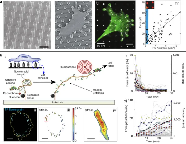
Cell-matrix connections transmit stresses to the ECM and are important in many physiolog- ical processes such as cell migration, proliferation, and differentiation. Cell-matrix connections can be classified into three different groups, as illustrated in Fig.1.3(b).

• Nascent adhesions(NAs) locate at the edge of a cell protrusion by nucleating three to six transmembrane proteins called integrins. NAs are dynamically coupled to the poly- merizing branched actin network.

• Focal adhesions(FAs) mature from a small number of nascent adhesions and these stable FAs are important for regulating cell adhesion and motility. FAs typically can be highly dynamic assemblies and thus the cell can change its shape and persistently migrate through ECM [111,112].

• Fibrillar adhesions(FBs) are developed from the maturing focal adhesions by growing their size and changing their protein composition [113,114]. Fibrillar adhesions are typically large adhesions in protrusions and the cell body and represent the endpoint in terms of adhesion maturation [115].

Various types of ECM can serve as substrate for cell adhesion [119]. Invivo, the native ECM of one cell can be other cells, tissues or organs, illustrated in Fig.1.3(c-i) [116]. Recently, to study properties and behaviors of cells, many artificial ECMs have been designed and fabricated, for example, beds of microneedles to isolate mechanical force [117] and poly- acrylamide hydrogels to study the traction force [118], illustrated in Fig.1.3(c-ii, c-iii), respectively.

(36)

Nucleus

Tight junctions Adherens junctions Desmosomes

Gap junctions

Actin Intermediate

laments

Occludin Claudins

Cingulin Paracingulin

JAM Nectin

a b

c 580/605-nm beads

Protein coating ii iii

i

Figure 1.3:Extracellular structures. (a) Four types of cell-cell conjunctions, gap junctions, tight junctions, adherens junctions, and desmosomes. (b) Three different types of cell-matrix conjunctions are classified into nascent adhesions, focal adhesions, and fibrillar adhesions according to the different levels of traction forces. Each of cell-cell and cell-ECM conjunctions is connected to the cytoskeleton inside of cells and thus the conjunction can transfer forces from cytoskeleton to ECM. (c) Extracellular native and artificial matrix. (c-i) Scanning electron micrograph demonstrates a native ECM, a tissue from the cornea of a rat. (c-ii) Artificial beds of microneedles to isolate mechanical force and collagen fibers matrix to learn cell migration. Space bar:10µm. (c-iii) Artificial substrates to be used for traction force microscopy. The beads and protein are put on the top of substrates. Space bar:30µm. (Figure (a) adapted from S. Sluysmans et al., 2017 [114]. Figure (b) adapted from Z. Sun et al., 2016 [109]. Figure (c-i) taken from B. Alberts et al., 2002 [116]. Figure (c-ii) taken from J. L. Tan, et al., 2003 [117]. Figure (c-iii) adapted from H. Colin-York et al., 2017 [118].)

A general principle for measuring the cellular forces is that a displacement field generated by the forces in the extracellular environment is first measured by using a microscopy technique and then the forces are calculated from the displacement field by using a given mechanical model. In the next section, we briefly introduce the imaging methods and mechanical models used in this context.

1.2.2 Mechanical models and imaging techniques

The CSK and extracellular structures typically are solid materials. These solid materials can be deformed by the motility-driving forces on CSK or the external forces applied on them.

The relationship between forces and deformation is called a material constitutive equation or a mechanical model. For solid elastic materials, this relationship can be defined by relating

(37)

1.2. Background information on measurement of cellular forces 11 the stressσ, the force per unit area, and strain, the fractional change in the length of a material.

a b

F

F F F

Linear

Nonlinear

Fibrous

Uniaxial tension Shear rheology AFM Beam bending

d

c i

ii

iii

i ii iii iv

Figure 1.4:Mechanical models and imaging techniques. (a) Mechanical models relating the force and displacement. (a-i) Simple relationship between stress and strain in linear materials with a constant Young’s modulus. (a-ii) The non-linear model can be also employed in measurement of cellular forces. (a-iii) The complex ECM can be described by an anisotropic and nonlinear model.

(b) Young’s modulus (E) represents the stiffness of solid materials, with units of Pa. Different types of cells have different Young’s moduli. (c) Under different types of loading, the equations of Young’s modulus can be written in different forms, for example, the forms of uniaxial tension, shear rheology, loading from atomic force microscopy (AFM), and beam bending shown in (c-i to c-iv).

(d) Imaging techniques for conducting biomechanical tests in different length scales. Imaging techniques, transmission electron microscopy, atomic force microscopy, scanning electron microscopy, fluorescence microscopy, optical microscope, and micro-CT are employed from the biomolecules to organs.

(Figure (a, c) adapted from J. M. Barnes et al., 2017 [96]. Figure (b) taken from W.

J. Polacheck et al., 2016 [120]. Figure (d) taken from C. T. Lim et al., 2006 [121].) The simplest mechanical model is linear elasticity. Here, stress is linearly related to the strain, illustrated in Fig.1.4(a-i), and the constant coefficient between the stress and strain is called Young’s modulusE. The different types of materials have different Young’s moduli, illustrated in Fig.1.4(b). Typical values are, for example, a Young’s modulus ofE ≈10 Pa for mucus and E ≈ 1 GPafor bone. For an elastic material, the equation allowing one to determine the Young’s modulus depend on the types of loading, for example, uniaxial tension, shear loading, loading from atomic force microscopy (AFM), and beam bending illustrated in Fig. 1.4(c-i to c-iv), respectively. The mechanical model can also be a non- linear relationship, illustrated in Fig.1.4(a-ii). The usual non-linear models include plasticity

(38)

and viscoplasticity. To model the complex structure of the ECM, one can also employ an anisotropic model, in which the anisotropy depends on the direction, illustrated in Fig.1.4 (a-iii).

We have introduced mechanical models for the CSK and extracellular structures. To calculate the forces that cells exert on these structures, we also need to measure the material displacements. Due to the fact that these structures are typically microscopically small, the displacement needs to be obtained by using a microscope or related imaging techniques.

Here, we briefly introduce several techniques to take images at different length scales, illustrated in Fig.1.4(d) [121] and the techniques include transmission electron microscopy (TEM), atomic force microscopy (AFM), scanning electron microscope (SEM), optical microscopy (includes fluorescence microscopy), and computer tomography. For example, to visualize the biomolecules of the cytoskeleton with sizes in thenmrange AFM, TEM, and fluorescence microscopy are required. Cells with sizes in theµm range can be visualized with AFM, TEM, SEM, optical microscopy, and fluorescence microscopy. Fluorescence microscopy utilizes the characteristic emissions of excited fluorophores, for example, fluores- cent proteins [122] and this microscopy technique has been widely employed to study cellar forces, for instance with traction force microscopy [118]. In the following section, we will introduce several special approaches to measure such cell-generated forces.

1.2.3 Measurement methods of cell-generated forces

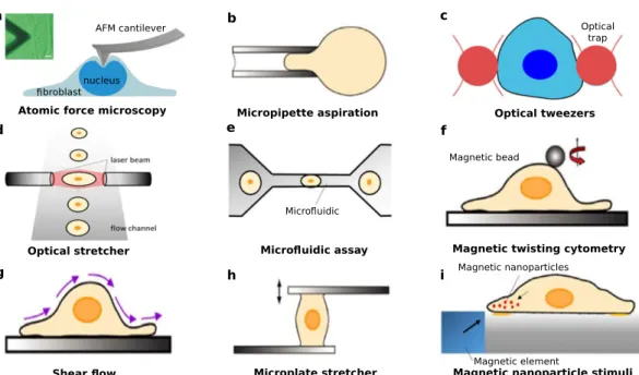
Over the past 50 years, various methods have been developed to measure the cell-generated forces. Here, we briefly introduce methods for measuring forces on a single cell and methods for measuring forces at cell-ECM connections.

1.2.3.1 Methods for measuring the mechanical behavior of a single cell

To study the mechanical response of a single cell, the cell is often subjected to an external loading. Under this load, the deformation of the cell can be measured and forces can be calculated by using a constitutive law. According to the different types mechanical devices, the methods [123,124] can be divided into the following categories:

• Atomic force microscopy(AFM) can be used to locally probe the mechanical response of cells. A schematic view of AFM is shown in Fig.1.5(a) and the minute displacement of the cantilever can be measured by using a high-resolution scanning probe microscopy.

AFM not only can measure the mechanical response of the cell, but also can provide a three-dimensional surface profile [127].

• Micropipette aspirationis a technique to deform one cell by using a pipette in a solution. The cell is partially aspirated into a glass pipette, illustrated in Fig.1.5(b), and the forces on the cell can be calculated by using a model related to the suction pressure [128].

• Optical tweezersutilize a highly focused laser beam acting on colloidal particles to provide a force on cells, illustrated in Fig.1.5(c). These instruments have been widely employed to measure the forces on molecules and cells [129,130].

• Theoptical stretcher is a contact-free measurement tool. A dual-beam optical trap is employed to deform the cells, which are in a flow channel, illustrated in Fig.1.5(d).

(39)

1.2. Background information on measurement of cellular forces 13

nucleus broblast

AFM cantilever

Atomic force microscopy Micropipette aspiration

Optical trap

Magnetic bead

Micro uidic

Magnetic element Magnetic nanoparticles

Optical tweezers

Optical stretcher Micro uidic assay Magnetic twisting cytometry

Shear ow Microplate stretcher Magnetic nanoparticle stimuli

a b c

d e f

g h i

Figure 1.5:Schematic different methods for measuring forces on a single cell.

(a) Atomic force microscopy (AFM). (b) Micropipette aspiration. (c) Optical tweezers. (d) Optical stretcher. (e) Microfluidic assay. (f) Magnetic twisting cytometry. (g) Shear flow. (h) Microplate stretcher. (i) Magnetic

nanoparticle-based stimuli. (Figure adapted from M. Unal et al., 2012 [95] with source material from S. Suresh, 2007 [123]; G Bao et al., 2003 [124]; H. Milting et al., 2014 [125] and F. D. Modugno et al., 2019 [126].)

• Themicrofluidic assayis a technique to analyze the mechanics of a cell by using fluid pressure. When fluid is flown one tube into a constriction, the pressure is increased and the cells can be deformed by the fluid.

• Magnetic twisting cytometryuses ferromagnetic microbeads to apply a twisting shear stress on cell surface receptors [131].

• Application of ashear flowto a cell that is adhered to a substrate can produce a deformation of the cell. The mechanical properties of the cell are studied by using a mechanical model.

• Themicroplate stretcheris a technique to stretch a cell by using a rigid glass micro-plate at the bottom and a flexible plate at the top [132] because the cell can adhere to the bottom and top microplates.

• Magnetic nanoparticle-based stimuliis a technique that relies on the displacement of magnetic nanoparticles deposited on the cell membrane or injected into the cell by using a magnetic field.

1.2.3.2 Methods for measuring forces of cell-ECM connections

Many approaches for quantifying cellular mechanics do not rely on external force applications. Such techniques include those for measuring the forces on cell-ECM connections, beds of microneedles, DNA hairpin force sensors, and traction force microscopy [96]. We mainly introduce the method based on beds of microneedles and DNA hairpin force sensors in this section. Traction force microscopy will be introduced in the next section.