Hybrid simulations of Titan’s plasma interaction: Case studies of Cassini’s

Hybrid simulations of Titan’s plasma interaction: Case studies of Cassini’s

T9, T63 and T96 flybys

I n a u g u r a l - D i s s e r t a t i o n zur

Erlangung des Doktorgrades

der Mathematisch-Naturwissenschaftlichen Fakultät der Universität zu Köln

vorgelegt von von Moritz Feyerabend

aus Wedelheine

Köln, 2016

(Gutacher) Prof. Dr. Bülent Tezkan

Tag der mündlichen Prüfung: 31.05.2016

Summary

In this thesis, we apply numerical simulations by means of the hybrid code A.I.K.E.F.

(Adaptive Ion-Kinetic Electron-Fluid) to study the interaction of Saturn’s magnetospheric plasma as well as the solar wind with Titan’s ionosphere. The composition of Titan’s ionosphere is represented by a 7-species model. The ionosphere is generated by a realis- tic wavelength dependent photoionization model of the main neutral species N

, CH

and H

. We also included elastic ion-neutral collisions of the impinging plasma with Titan’s neutral atmosphere to our model as well as a network of the most important chemical reactions of the ionosphere that converts between the ion species.

In the first part of the thesis we investigate the physical processes that lead to the detection of ’split signatures’ in the ion densities during several crossings of the Cassini spacecraft through Titan’s mid-range plasma tail (T9, T63, and T75). During each of these flybys, the Cassini Plasma Spectrometer observed Titan’s ionospheric ion population twice; i.e., the spacecraft passed through two spatially separated regions where cold ions were de- tected. Our simulation results show that the filamentation of Titan’s tail is a common feature of the moon’s plasma interaction. The transport of ionospheric ions of all species from the ramside to the moon’s wakeside generates a cone-like structure on the down- stream side, that contains a region of reduced density. In addition, light (mass 1-2 amu) ionospheric species are driven radially outwards by pressure gradients in the ionosphere and escape along draped magnetic field lines, forming a parabolically shaped filament structure which is mainly seen in planes that contain the upstream magnetospheric mag- netic field and the upstream flow direction. Our results imply that the detections of split signatures during T9, T63 and T75 are consistent by Cassini penetrating through parts of these filament structures.

In the second part of the thesis we study Titan’s plasma interaction with the solar wind

during the Cassini T96 flyby. The T96 encounter marks the only observed event of the

entire Cassini mission where Titan was located in the supersonic solar wind in front of Sat-

urn’s bow shock. We show that the large-scale features of Titan’s induced magnetosphere

during T96 can be described in terms of a steady-state interaction with a high-pressure

solar wind flow. About 40 minutes before the encounter, Cassini observed a rotation of

the incident solar wind magnetic field by almost 90 degrees. We provide strong evidence

that this rotation left a bundle of fossilized magnetic field lines in Titan’s ionosphere that

was subsequently detected by the spacecraft.

Zusammenfassung

In dieser Arbeit benutzen wir numerische Simulationen auf Basis des Hybrid Codes A.I.K.E.F. (Adaptive Ion-Kinetic Electron-Fluid), um die Plasma Wechselwirkung von Titans Ionosphäre mit Saturns magnetosphärischem Plasma als auch dem Sonnenwind zu untersuchen. Die Zusammensetzung von Titans Ionosphäre wird durch ein Modell mit 7 Spezies repräsentiert. Die Ionosphäre wird durch ein realistisches, wellenlängenab- hängiges Photoionisationsmodell der neutralen Hauptspezies N

, CH

und H

generiert.

Desweiteren haben wir elastische Ionen-Neutral Kollisionen des anströmenden Plasmas mit Titans Neutralatmosphäre zu unserem Modell hinzugefügt sowie ein Netzwerk der wichtigsten chemischen Reaktionen der Ionosphäre welches für die Umwandlung der Spezies untereinander sorgt.

Im ersten Teil dieser Arbeit untersuchen wir die physikalischen Prozesse die zur Beobach- tung sogenannter ’split signatures’ in den Ionendichten von mehreren Vorbeiflügen (T9, T63, T75) der Cassini Sonde durch Titans mittel-entfernten Magnetosphärenschweif füh- rten. Während jedem dieser Vorbeiflüge registrierte das Cassini Plasma Spektrometer Titans Ionenpopulation zwei mal: i.,e., das Raumfahrzeug passierte zwei räumlich ge- trennte Regionen in denen kalte Ionen beobachted wurden. Unsere Simulationsergeb- nisse zeigen, dass die Filamentierung von Titans Magnetosphärenschweif eine allgemeine Eigenschaft von Titans Plasmawechselwirkung ist. Der Transport von ionospärischen Io- nen aller Spezies von der Anströmseite zur stromabgewandten Seite erscha ff t eine zylin- derartige Struktur stromabwärts, die eine Region reduzierter Dichte umschliesst. Ausser- dem werden leichte Ionen in der Ionospäre (Masse 1-2 amu) durch Druckgradienten radial auswärts gerichtet beschleunigt und bewegen sich dann entlang drapierter Magnetfeldlin- ien. Dies führt zur Ausbildung von parabolisch geformten Filamenten, welche hauptsäch- lich in Ebenen gesehen werden können die den Magnetfeldvektor und die Richtung des Anströmplasmas enthalten.

Im zweiten Teil der Arbeit untersuchen wir Titans Plasmawechselwirkung mit dem Son-

nenwind während des T96 Vorbeifluges von Cassini. Die T96 Begegnung stellt den einzi-

gen Zeitpunkt der gesamten Cassini Mission dar, in dem Titan im überschall schnellen

Sonnenwind vor Saturns Bugstosswelle eingebettet war. Wir zeigen, dass die gross-

skaligen Eigenschaften von Titans induzierter Magnetospähre während T96 konsistent

sind mit dem Bild einer quasi-stationären Wechselwirkung Titans mit einem Sonnenwind

der einen hohen dynamischen Druck hat. Ungefähr 40 Minuten vor seinem Vorbeiflug

detektierte Cassini dabei eine Rotation des anströmenden Sonnenwindmagnetfeldes um

fast 90 Grad. Wir liefern starke Hinweise, dass diese Rotation ein Bündel von fossil-

isierten Magnetfeldlinien in Titans Ionosphähre hinterlassen hat, welche in der Folge von

der Sonde beobachtet wurden.

Contents

Summary v

Zusammenfassung vii

1 Introduction 1

2 Titan’s Plasma Environment 7

2.1 Saturn’s Magnetospheric Structure . . . . 7

2.1.1 Coordinate System . . . . 11

2.1.2 Dynamics of the Magnetodisk . . . . 12

2.2 Titan’s Atmosphere . . . . 21

2.3 Titan’s Plasma Interaction . . . . 23

2.4 Fossilized Magnetic Fields at Titan . . . . 28

3 Simulation Model 33 3.1 Hybrid Model A.I.K.E.F. . . . 33

3.2 Numerical Implementation . . . . 36

3.3 Titan ionosphere model . . . . 38

3.4 Other Titan simulation models . . . . 42

4 Split Signatures in Titan’s tail 45 4.1 Introduction . . . . 45

4.2 Simulation Setup and Numerical Parameters . . . . 49

4.3 Run #1: Voyager-type upstream conditions . . . . 52

4.3.1 Run #1: Collisions and ∇P

removed . . . . 54

4.4 Run #2: T9-type upstream conditions . . . . 56

4.5 Run #3: T63-type upstream conditions . . . . 62

4.5.1 T75 split signatures . . . . 63

4.6 Summary . . . . 64

5 Titan in the Supersonic Solar Wind 67 5.1 Introduction . . . . 67

5.2 Simulation Parameters . . . . 72

5.3 Model Results and Discussion . . . . 75

5.4 Concluding Remarks . . . . 80

6 Summary and Outlook 81 6.1 Outlook . . . . 83

Bibliography 85

Acknowledgements 97

Erklärung 99

1 Introduction

Saturn’s moon Titan has been in the spotlight of scientific interest ever since its discov- ery by Christiaan Huygens in 1655. One of the reasons for that lies in its thick neutral atmosphere, the presence of which has been know from earthbound spectral observations since the early 1940s. The flybys of Pioneer 1 and Voyager 1 in the late 1970s and early 1980s further sparked the interest in the moon, as they confirmed that Titan’s atmosphere is mainly composed of nitrogen. Titan is the only other body in the Solar system except Earth, that has a nitrogen-based atmosphere. It is also the second-largest moon (after Ganymede) in the entire Solar system with a radius of R

= 2575 km, which puts it even before Mercury regarding the size. The exploration of Titan has been declared one of the major scientific aims of the NASA / ESA Cassini mission that was launched in 1997. Since its arrival in the Saturnian system on 01 July 2004, the Cassini spacecraft has performed

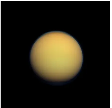
Figure 1.1: Natural color view on Titan from a distance of 191000 km. The picture was taken by Cassini’s Imaging Science Subsystem (ISS) on 30 January, 2012. A thick haze layer of organic compounds in the lower atmosphere gives Titan a yellow-orange color.

Credit: NASA webpage.

117 visits to Titan at the time of writing

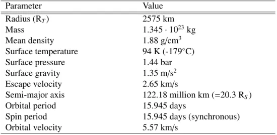
. One of the prime moments of the Cassini mis- sion was the landing of the Huygens landing probe, that provided in-situ measurements of Titan’s atmosphere during its decent on 14 January 2005. Titan therefore states the most distant celestial body where a human-made object has landed. A summary of Titan’s main physical and orbital parameters is provided in table 1.1.

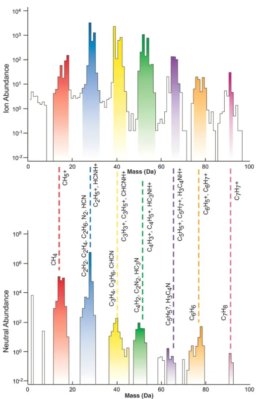
The data gathered by Cassini has revealed that Titan’s atmosphere is the host of a very complex chemistry network which is fueled by nitrogen and methane. The organic com- pounds that are created by this chemistry network are found in a very broad mass range from 1 to ∼10000 amu all over Titan’s atmosphere. At low altitudes, the heaviest species are found as aerosols that form a thick haze layer which gives Titan it’s characteristic yellow-orange appearance (see figure 1.1). Titan’s surface is covered with a crust of frozen water ice and lakes of liquid methane that condensates as a result of the atmo- spheric climate processes. Solar radiation and energetic particles create ionize the neutral atmosphere at high altitudes, which leads to the formation of an extended ionosphere around the moon. Titan is therefore very similar in its atmospheric structure to Earth.

Parameter Value

Radius (R

) 2575 km

Mass 1.345 · 10

kg

Mean density 1.88 g / cm

Surface temperature 94 K (-179

C)

Surface pressure 1.44 bar

Surface gravity 1.35 m / s

Escape velocity 2.65 km / s

Semi-major axis 122.18 million km ( = 20.3 R

)

Orbital period 15.945 days

Spin period 15.945 days (synchronous)

Orbital velocity 5.57 km / s

Table 1.1: Main physical and orbital parameters of Saturn’s largest moon, Titan.

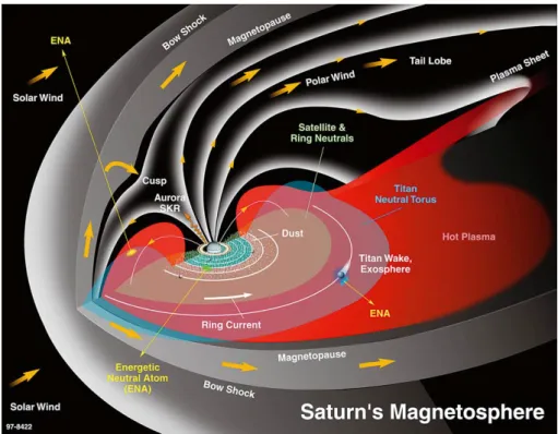
While Titan’s atmospheric and surface processes are already scientifically very interest- ing, the plasma interaction between Titan and Saturn’s magnetospheric plasma has also been a major topic of the Cassini mission. Since the moon’s orbital velocity is much smaller than the ambient plasma flow, Titan gets constantly overtaken by Saturn’s magne- tospheric plasma. Similar to Mars and Venus, Titan does not possess a noticeable intrinsic or induction-generated magnetic field (Wei et al. 2010) so that the moon’s atmosphere and ionosphere acts as an obstacle to the impinging plasma flow. As a result, the magnetic field lines drape around the moon’s ionosphere which leads to the formation of a char- acteristic perturbation pattern of the magnetic field and plasma flow on the ram side and downstream of the moon (called induced magnetosphere). However, Titan’s plasma in- teraction is unique among that of other non-magnetized bodies in the solar system due to its highly variable plasma environment. Over ten years of observations from Cassini have established the picture of a highly dynamic structure of Saturn’s magnetosphere (see figure 1.2) that is defined by the influences of the solar wind and its internal rotation. The

1

The T118 flyby is scheduled for 04 April 2016

1 Introduction mass loading of Saturn’s magnetosphere with particles originating from Enceladus water plumes leads to the formation of a sub-corotating equatorial plasma sheet that distorts Saturn’s dipolar magnetic field structure over the scale of the magnetosphere. In addition, the plasma sheet has been observed to show an oscillatory vertical motion. As a result, the local plasma and magnetic environment of the magnetosphere changes as a function of the distance to the equatorial plasma sheet. Titan orbits around Saturn at a distance of about 20.3 Saturn radii, which puts it in the outer regions of Saturn’s magnetosphere. In this re- gion the dynamical e ff ects and the distorted structure of Saturn’s magnetosphere are most pronounced. If the solar wind dynamic pressure is large enough it is even possible that Titan is located in Saturn’s magnetosheath region or outside of Saturn’s magnetosphere in the solar wind. Titan is therefore extremely susceptible to changes in its ambient plasma environments at its location which in turn is reflected by Titan’s plasma interaction with the ambient magnetosphere.

Figure 1.2: Schematic of the large scale structure of Saturn’s magnetosphere in the solar wind. Figure from Krimigis et al. (2004).

At the nearing end of the Cassini mission in 2017, culminating into the controlled descent of the spacecraft into Saturn’s upper atmosphere during its final phase, a tremendous amount of research has been devoted and published towards many aspects of Titan’s sur- face, atmosphere, ionosphere, chemistry and plasma interaction. The general structure of Titan’s plasma interaction under the variable nature of its plasma environment is known to the most part and many numerical models have been developed that verified this knowl- edge by reproducing observational data with computer simulation.

In this study we therefore focus on some of the unique observations and flybys made by

Cassini that have not yet been explained at all or in a satisfactory manner. In particular

we focus on the T9, T63, T75 and T96 Titan flybys of Cassini, which were all exceptional

in a certain way. The T9, T63 and T75 flybys were encounters where Cassini crossed at a great distance through Titan’s downstream magnetotail region. A remarkable obser- vation that was only made during these encounters was the detection of a ’split’ tail: a spatially separated double observation of a cold ion population that originated from Ti- tan’s ionosphere. Our goal in this thesis is to get a better understanding of the physical processes that lead to the detection of these ’split signatures’ and whether or not this is an omnipresent feature of Titan’s plasma interaction that might have been missed during other flybys.

The T96 flyby is a truly unique encounter as it constitutes the only time of the entire Cassini era where Titan was embedded in the supersonic solar wind in front of Saturn’s bow shock during a time of extreme solar wind dynamic pressure. This encounter has not yet been subject to any modeling attempt so far. We examine if the large-scale ob- servations of Titan’s induced magnetosphere can be described in terms of a steady state interaction with the high pressure solar wind. Since the dynamic pressure of the solar wind is loaded with some uncertainty for this encounter, we use it as a free parameter to find a setting that produces numerical results which are in agreement with magnetic field and electron density measurements. In addition we investigate the e ff ects of the variable mag- netic environment on Titan’s magnetic signature during this encounter. We also analyze the contribution of fossilized magnetic field lines from an upstream magnetic regime prior to the encounter to the small scale magnetic pattern inside Titan’s ionosphere. Fossilized magnetic field lines can be understood as the imprint of a varying upstream magnetic con- figuration on Titan’s ionosphere, in some analogy to the growth-rings of trees.

To address these problems we perform numerical simulations of Titan’s plasma interac- tion using a hybrid model. A hybrid model treats ions as kinetic particles and electrons acts as a massless charge neutralizing fluid. The hybrid approach is able to resolve e ff ects that arise due to the gyrating motion of ions in a magnetized plasma flow. At Titan these e ff ects cannot be neglected since the local gyro radius is always at least comparable to the moons radius, which leads to a noticeable asymmetrization of its induced magnetosphere.

Fluid models that treat ions as a fluid as well are therefore limited in their ability to cor- rectly represent the relevant physics near Titan. The model of Titan’s ionosphere that is used in this thesis has been significantly improved compared to previous studies (Simon et al. 2006b). We have included a realistic model of the photoionization of Titan’s neutral atmosphere and represent the relevant ion species of Titan’s ionosphere with a 7-species model that also includes elastic collisions and the most important chemical reactions.

This thesis is structured as follows: in chapter 2 we give the theoretical background that is needed to understand the complex nature of Titan’s interaction with the highly variable plasma environment of Saturn’s magnetosphere. We continue with a brief description of the hybrid code A.I.K.E.F. (Adaptive-Ion-Kinetic-Electron-Fluid) and the representation of Titan’s ionosphere and chemistry network in chapter 3. Our results are presented in chapter 4 and 5:

• In chapter 4 we use our model to study the fine structure of the density distribution

in Titan’s downstream magnetotail region. We study the ion transport mechanisms

that lead to the formation of this fine structure as well as the spatial restrictions that

are placed on them by the relative orientation of the upstream flow direction and

background magnetic field. We use our findings to compare hybrid model results

of the T9 and T63 flyby against density measurements obtained by Cassini and give

1 Introduction reasons for the unexpected spatially separated detection of cold ionospheric ions during those encounters.

• Chapter 5 focuses on Titan’s interaction with the supersonic solar wind during Cassini’s unique T96 flyby. We investigate the impact of the variable solar wind environment on Titan’s induced magnetosphere structure as well as the contribution of fossilized magnetic fields to the magnetic observations around closest approach of the spacecraft.

Finally, we summarize the major findings of this thesis and give a brief outlook on future

projects in chapter 6.

2 Titan’s Plasma Environment

In this chapter we give the theoretical background and current knowledge of Titan’s plasma environment and its interaction with Saturn’s magnetospheric plasma. The general structure and dynamic behavior of Saturn’s outer magnetosphere near Titan is described in section 2.1. In section 2.2 we describe the unique features of Titan’s atmosphere and its rich nitrogen fueled chemistry. Finally we explain the general aspects of Titan’s plasma interaction in section 2.3 and give further insight into the phenomenon of fossilized mag- netic fields in Titan’s ionosphere in section 2.4.

2.1 Saturn’s Magnetospheric Structure

Saturn’s magnetosphere is generated by its intrinsic dipolar magnetic field. A peculiarity of Saturn’s dipole moment compared to other planets is that is almost perfectly aligned with the planets rotation axis with a tilt of less than 0.1

and an o ff set of 0.036 R

(Bur- ton et al. 2010). The planet’s magnetic field has a surface strength of 21136 nT (Burton et al. 2010). Saturn’s magnetosphere is filled with neutral particles that emanate from the planet itself, its icy moons (e.g. Enceladus, Rhea, Dione) and the ring system via sput- tering and atmospheric losses (Arridge et al. 2011c). The neutral particles then become ionized through photoionization, electron impact and charge exchange processes. Over- all, Saturn’s magnetosphere is dominated by neutral particles, which have been found to outnumber ions by a factor of 10-100 (Arridge et al. 2011). The major source of particles in the magnetosphere are the water plumes of Saturn’s moon Enceladus (Hansen et al.

2006). The dominant ion species in Saturn’s magnetospheric plasma thus consists of wa- ter group ions (O

, OH

, H

O

, H

O

) and protons H

.

Enceladus is located in the inner magnetosphere at a distance of 3.95 Saturn radii (equa-

torial radius R

= 60.268 km). This has severe consequences on the general structure

of Saturn’s magnetosphere. The magnetospheric plasma corotates with the planet and

contains the frozen-in magnetic field. Ions that are inserted into the system near Ence-

ladus move at least with the speed of Enceladus orbital velocity, which is 12.6 km / s and

slower than the corotational velocity of ∼ 26 km / s. The ions are then accelerated by

the convective electric field until their guiding center reaches nearly corotational velocity

(also know as ’pick-up’ process). However, the distance at which the centrifugal forces

acting on the corotating plasma and Saturn’s gravitational force cancel each other lies at

a distance much lower than Enceladus orbit. Therefore, the plasma that is generated by

the plumes of Enceladus is driven radially outward from Saturn due the outwards point-

ing centrifugal force and the arising plasma pressure gradients. This outwards pointing

plasma flow leads to a large scale deformation of the magnetic field in the outer region of

Figure 2.1: Side-on view of Saturn’s magnetodisk structure. The figure illustrates Sat- urn’s (grey circle) magnetic field configuration (red lines) when the observer-Saturn line is perpendicular to Saturn’s magnetic moment M. In the northern (labeled L

) and southern (labeled L

) magnetic lobes the field lines are highly stretched and possess strong radial components. In the narrow current sheet region of the magnetodisk around the magnetic equator (labeled Sh, green area), the magnetic field is still quasi-dipolar and nearly an- tiparallel to Saturn’s rotation axis. Titan’s orbit in this idealized picture is indicated by the dashed black line. Figure from Simon et al. (2010).

Saturn’s magnetosphere. The azimuthal current system that is associated with the coro- tating plasma stretches Saturn’s magnetic field from a dipolar shape to a deformed shape that is characterized by highly stretched magnetic field lines above and below the mag- netic equator. This structure of the magnetosphere is referred to as the ’magnetodisk’ (Ar- ridge et al. 2007) of Saturn’s magnetosphere. The extent of the magnetodisk is balanced by the inwards pointing j × B forces exerted on the azimuthal currents of the corotating plasma. The azimuthal currents become stronger with increasing distance to the planet, due to the increasing azimuthal velocity of the corotating plasma. The general structure of Saturn’s magnetosphere can be separated into three main parts: a dipolar field region in the inner magnetosphere until 5 R

, a quasi-dipolar field region with a weak current sheet in the middle magnetosphere from about 5 to 12-15 R

, and finally the disk-like region with highly stretched field lines and a strong current sheet in the outer part of the magnetosphere (Arridge et al. 2007).

A sketch of the magnetodisk structure is provided in figure 2.1. In the northern mag- netic lobe, the magnetic field is mainly pointing radially away from Saturn, whereas in the southern lobe the field is oriented mainly towards the planet. The degree of how much the field lines are stretched towards / away from the planet can be calculated by means of the stretch angle

Str = arctan B

B

!

, (2.1)

where B

and B

are the magnetic field components in TIIS coordinates (see section 2.1.1).

A positive stretch angle is therefore an indication of a location in the northern magnetic

lobe, while a negative stretch angle indicates a position in the southern magnetic lobe.

2.1 Saturn’s Magnetospheric Structure

Figure 2.2: Illustration of the stretch angle. The figure shows Saturn’s stretched magnetic field lines of the magnetodisk in a meridional plane ( = yz-plane of the TIIS system). The y axis points towards Saturn and the z axis is parallel to Saturn’s magnetic moment. The B

component of the magnetic field is negative above the magnetic equator and positive below the magnetic equator. Therefore the stretch angle Str = arctan( − B

/B

) is positive for locations in the northern magnetodisk lobe and negative for locations in the southern magnetodisk lobe. At the magnetic equator where B

= 0, the stretch angle vanishes.

Figure from Simon et al. (2010)

Figure 2.2 illustrates the stretch angle in case the current sheet coincides with the mag- netic equator. The value of the stretch angle provides a measure of how much the field lines are stretched at an observers position. A high stretch angle value is therefore an indication of a great distance to the magnetodisk’s current sheet.

The magnetodisk is not only characterized by the highly stretched field lines in the lobes,

it also shows a deformation of the field lines in the corotational direction. The equato-

rial current sheet is strongly coupled to Saturn’s ionosphere via field aligned Birkeland

currents (magnetosphere-ionosphere coupling, Hill (1979)). These currents transfer an-

gular momentum from Saturn’s ionosphere into the current sheet in order to accelerate

the plasma to corotational speeds. However, this process is limited by the finite Petersen

conductance of Saturn’s ionosphere. Therefore the magnetosphere-ionosphere coupling

cannot provide the necessary angular momentum that is needed to enforce a rigid corota-

tion of the magnetospheric plasma throughout the whole of the magnetosphere. Instead,

strict corotation of the plasma is found only in the inner magnetosphere . With increasing

distance from Saturn, the plasma is found to subcorotate at about 50-80% of the ideal

corotation speed (Thomsen et al. 2010). In the outer magnetosphere (> 15 R

) a sat-

uration is reached, where the azimuthal velocity of the plasma remains nearly constant

(Arridge et al. 2011c). At the orbital distance of Titan, the full corotational speed would

be ∼ 200 km / s, however the average plasma speed is found to be in the range of 120 − 160

km / s (e.g Wilson et al. (2010)). Frozen-in field lines in the equatorial current sheet are

Figure 2.3: Illustration of the sweepback angle. The figure shows how Saturn’s magnetic field lines are bent back with respect to a strictly corotating meridional plane as a result of the corotational lag in Saturn’s magnetodisk current sheet. Plot (a) shows the xz-plane of the TIIS system, plot (b) shows a xy-cut above (z > 0) and plot (c) a xy-cut below Titan’s orbital plane. When the magnetic field lines are bent back with respect to a x = const plane, the sweepback angle Sw = arctan(−B

/B

) is negative both above and below the magnetic equator. Figure from Simon et al. (2010).

therefore bent back with respect to a strictly corotating meridional plane (see figure 2.3).

The magnitude of this sweepback can be measured with the sweepback angle Sw = arctan −B

B

!

. (2.2)

With this definition, the sweepback angle is negative for swept back magnetic field lines for locations both north and south of the magnetic equator. Consequently, for a scenario of swept forwards field lines that indicate a super corotational plasma flow, the sweep angle would be positive. Observations of positive sweep angles have been occasionally observed near the dusk flank of Saturn’s magnetosphere (Bertucci 2009).

Particles at high latitudes experience a gravitational pull towards the equatorial region,

where, balanced by the centrifugal force, they are then confined to the plasma sheet. The

thickness of the plasma sheet is on the order of 1-2 R

(Arridge et al. 2011a), with the

heavy ions having a smaller scale height than light ions (Thomsen et al. 2010) due to

the di ff erent masses. Therefore, light ions (protons, hydrogen) are found to dominate the

plasma composition in the regions of Saturn’s magnetic lobes whereas heavy ions (water

group) will dominate in the equatorial current sheet. The plasma beta β = 2µ

nkT /B

,

which is the ratio between thermal pressure and magnetic pressure, shows a similar behav-

ior with a high beta value in the plasma sheet, and a lower beta value in the magnetodisk

2.1 Saturn’s Magnetospheric Structure lobes (Achilleos et al. 2014).

In combination with the magnetic structure of Saturn’s magnetosphere, two main plasma regimes can be distinguished (Arridge et al. 2007): (a) a current sheet regime which is characterized by a dense, high beta plasma composition and a quasi-dipolar magnetic field configuration and (b), a lobe-type regime consisting of a more dilute low-beta plasma with stretched and swept-back magnetic field lines.

2.1.1 Coordinate System

Figure 2.4: Illustration of the Titan Interaction System (TIIS) used in this thesis. Also displayed are the orientations of the main upstream plasma parameters E

, B

and U

for idealized upstream conditions.

To be able to perform numerical simulations of Titan’s plasma interaction, a suitable co-

ordinate system that covers the simulation domain is needed. The rotating rest frame of

the moon on its orbit around Saturn constitutes a natural choice of coordinates that are

best suited to exploit the geometry of the plasma interaction. In the case of Titan, this

magnetosphere-moon-interaction system is called the Titan Interaction System (TIIS). In

the TIIS system, the x axis points in the direction of nominal corotation, which is identi-

cal to the direction of Titan’s orbital motion around Saturn. The y axis of the coordinate

system is pointing towards the center of Saturn, and the z axis is anti-parallel to Saturn’s

rotational axis. The origin coincides with the center of Titan. The coordinate system is

sketched in figure 2.4, where we assume idealized upstream conditions, i.e, the magnetic

field B

is aligned with the −z axis, the upstream flow direction is aligned with the x axis

and the convective electric field E

= −U

× B

points in the −y direction. However, for

the majority of Cassini Titan flybys these parameters were found to not fit this picture of

ideal plasma conditions very well, as we will see in section 2.1.2.

Another frame of reference that is frequently used to describe Saturn’s magnetosphere is the cylindrical polar Kronocentric Solar Magnetic (KSMAG) coordinate system (ρ,φ,z).

In this system the radial unit vector e

is pointing away from Saturn’s rotational axis, the azimuthal unit vector e

is pointing eastwards in the corotational direction and the vertical unit vector e

is aligned with the planets rotational axis. Note that the only di ff erence of this system to TIIS coordinates is a minus sign in the radial (y in TIIS) coordinate.

Another important set of parameters are the Saturn Local Time (SLT) and Subsolar Lati- tude (SSL) at the time of an encounter. These parameters define the exact location of the subsolar point in the TIIS system and therefore control the position and orientation of the ionosphere which is mostly generated through photoionization processes. They depend on Titan’s orbital status and the Saturnian season. An illustration of the parameters is given in figure 2.5. The SLT can assume values from 0 to 24 as Titan orbits around Saturn. If Titan is at 6 or 18 SLT, the ramside of the impinging magnetospheric plasma coincides with the nightside (6 SLT) or the dayside (18 SLT) of Titan ’s photogenerated ionosphere.

Due to the tilt of Saturn’s rotational axis with respect to the ecliptic, and therefore Titan’s orbit as well, the SSL varies from −26.7

to 26.7

depending on the Saturnian season.

Figure 2.5: Illustration of (a) Titan’s Saturn Local Time (SLT) and (b) Subsolar Latitude (SSL). The SLT denotes the orbital positions of Titan with respect to the sun. Due to the tilt of Saturn’s rotational axis, the subsolar point changes with the seasons.

2.1.2 Dynamics of the Magnetodisk

Given that Titan’s orbit lies within Saturn’s equatorial region, one might expect to observe current-sheet like plasma conditions at Titan at all times. However this was found to be the case only on average. During many Cassini flybys, Titan was actually found to be em- bedded in the plasma environment of the magnetodisk lobes. The reason for this is that Saturn’s magnetodisk is not a stationary system, but rather shows dynamic behavior on various timescales ranging from minutes to several years. These dynamics are induced by either internal processes of the Saturnian magnetosphere or other external factors, mainly the solar wind as well as the Saturnian seasons, and will be described in the following.

The first external process that influences the shape of Saturn’s magnetosphere is related to

the solar wind pressure and manifests in a day-night asymmetry of the magnetodisk struc-

2.1 Saturn’s Magnetospheric Structure

Figure 2.6: Sketch of the distortion of Saturns magnetosphere along the noon-midnight meridian during a) southern and b) northern summer. As a result of the solar wind press- ing against the magnetodisk’s current sheet from either below or above, the magnetodisk adopts a bowl-like shape. Figure taken from Arridge et al. (2008a)

ture: The impinging solar wind naturally tries to compress the dayside magnetosphere, counteracting the formation of the magnetodisk in the near-noon local time sectors. If the solar wind dynamic pressure is su ffi ciently high, the stand-o ff distance of Saturn’s magnetopause (where Saturn’s magnetic pressure is balanced by the solar wind dynamic pressure) is close enough so that the magnetopause currents e ff ectively suppress the for- mation of the magnetodisk. Instead a quasi-dipolar field configuration in the near noon time sectors is enforced, as opposed to the nightside and around dusk and dawn sectors, where the magnetodisk structure is not prevented at all. Arridge et al. (2008b) showed that the dayside formation of the magnetodisk can only prevail in times of low solar wind dynamic pressure, where the stand-o ff distance of the magnetopause is at 23R

or larger.

Since the solar wind dynamic pressure variations do not follow predictable processes, the timescale of the magnetodisk’s day-night asymmetry cannot be constrained with by fixed value and may change on a day-to-day basis.

The solar wind has a second impact on the magnetodisk’s structure which is also related

to the tilt of Saturn’s rotational (' magnetic) axis, and therefore to the Saturnian seasons.

Due to this tilt, the solar wind impinges at an angle of up to 26.7

(during the solstices) onto Saturn’s magnetic equator plane from either ’above’ or ’below’. This leads to a de- formation of the outer magnetodisk region into a basin- or bowl-like form (Arridge et al.

2008a), with the magnetic equatorial plane (where the radial magnetic field component B

changes sign) being displaced against the rotational equatorial plane. On average, Titan is therefore embedded in the region of the southern magnetodisk lobe during Saturn’s south- ern summer and in the northern magnetodisk lobe during Saturn’s northern summer. An illustration of the magnetobowl shape for the two seasons is shown in figure 2.6. Around the equinoxes, this e ff ect is much less pronounced, as the impacting angle of the solar wind with respect to the magnetic equatorial plane is close to zero during this time.

Even though Saturn’s magnetic moment and rotational axis are almost perfectly aligned, a number of oscillatory phenomena in the magnetic field and other plasma parameters act- ing on timescales near the planets rotation period of ∼ 10.7 have been observed in Saturn’s magnetosphere (e.g. Kurth et al. (2008), Khurana et al. (2009), Andrews et al. (2010)).

Near Titan, these periodicities are observed as a north-south oscillatory motion of the magnetodisk’s current sheet over the moon’s orbital plane, which is also referred to as the

’flapping’ of the magnetodisk (Arridge et al. 2008, Arridge et al. 2011b). E ff ectively this means that the plasma and magnetic conditions near Titan can show transitions between the magnetospheric environments of the northern and southern magnetodisk lobe as well as the magnetodisk current sheet on a timescale of ∼10 h. The reason for these oscillatory behavior of Saturn’s magnetosphere is still one of the major open question that has not yet been explained in a satisfactory way (e.g. Andrews et al. (2012), Southwood and Cowley (2014)).

An exemplary observation of a full cycle of such a current sheet sweep across Titan’s orbital position is given in figure 2.7, showing the magnetic field data obtained by the Cassini spacecraft during the T54 encounter on May 5, 2009 along with a sketch of mag- netodisk’s flapping motion at that time. During this encounter, the current sheet moved at least two times over Cassini’s position, accompanied each time with a transition of the magnetic environment from one lobe regime to the other. The intervals where Cassini is embedded in the magnetodisk lobe regions are about 5 h long, roughly half of the planetary rotation period. They are clearly identified by their characteristic magnetic sig- natures: B

> 0 in the southern magnetodisk lobe, B

< 0 in the northern lobe. Also the sweepback of the magnetic field is visible in the B

component in those intervals: B

> 0 in the southern lobe, B

< 0 in the northern lobe, see also figure 2.3. One of the current sheet sweeps is nearly coincident with Cassini’s closest approach to Titan. This illustrates that these types of internally induced dynamics of the magnetodisk are quite significant for the understanding of Titan’s plasma interaction, since they can disturb the upstream plasma and magnetic conditions on the timescale of a Cassini flyby.

The magnetic field observations depicted in figure 2.7 also show the last dynamic pro-

cess of the magnetodisk current sheet, which is also associated with the flapping motion

mentioned above. As can be seen in the time interval from 02:00-04:00 in figure 2.7, the

north-south motion of the current sheet does not necessarily need to be a smooth transi-

tion from one lobe regime to the other. Instead, the magnetic field can be accompanied

by short-scale ’jitter’ with periods up to 30 min. The occurrence of such short-scale fluc-

tuations of the magnetic field in the magnetodisk’s current sheet near Titan is in fact an

2.1 Saturn’s Magnetospheric Structure

Figure 2.7: Sketch of the current sheet (green shaded area) sweeping over Titan and

Cassini (C) during T54 (top figure, a-d) combined with the magnetic field observations

made by Cassini (bottom figure). The areas distinguished by the red lines and marked

with characters a, b, c, d in the magnetic data plot correspond to the four snapshots of

the magnetodisk’s state in the top figure. (a) Cassini and Titan are located in the southern

magnetodisk lobe region after a northward sweep of the current sheet (b) The recurring

current sheet sweeps back over Titan shortly after closest approach (c) The current sheet

has swept south past Titan and Cassini, putting both in the northern magnetodisk lobe

regime (d) The current sheet sweeps back again and is now located above Cassini, putting

the spacecraft again in the southern lobe. Figures from Simon et al. (2010).

omnipresent feature and has been observed multiple times by Cassini (e.g. figure 2 in Arridge et al. (2007), figure 7 in Simon et al. (2010)). The magnitude of the ’jittering’ in the current sheet can be comparable to the background magnetic field strength and even last for several hours, as evidenced during the T20 encounter (see figure 6 in Simon et al.

(2010)).

The picture of the magnetospheric conditions that arises near Titan (and generally in the outer magnetosphere at distances > 15 R

) is that of a highly disturbed magnetospheric environment. The various dynamic processes of the magnetodisk current sheet can change the conditions near Titan on timescales of minutes and may influence Titan’s plasma in- teraction significantly during a single Cassini flyby. For this reason, several classification schemes have been developed in the past in order to characterize the plasma environ- ment near Titan’s interaction region on an encounter-to-encounter basis, utilizing di ff erent Cassini instruments and the large data set of Titan flybys.

Using electron spectra obtained from the Cassini Plasma Science (CAPS) and Magne- tospheric Imaging Instrument (MIMI) instruments, Rymer et al. (2009) developed such a classification scheme for the encounters TA-T54. This scheme was later expanded up to the T84 flyby by Smith and Rymer (2014), which was the last Titan encounter where the CAPS instrument was still operational on board of Cassini. Observational data in a

±3 h window around closest approach is considered. The scheme by Rymer et al. (2009) distinguishes between four types of encounters based on the peak energy and flux density of the observed electron distribution: ’plasma sheet’ (high energy, high flux), ’lobe-like’

(high energy, low flux), ’magnetosheath’ (low energy, very high flux) and ’bimodal’ (su- perposition of cold and high energy electron populations). The specific criteria for each type are listed in table 2.1. Encounters that could not unambiguously be identified were marked as unclassifiable and those with more than one type identified, as mixed. A mixed classification typically indicates transition between plasma regimes over the course of an encounter. The combined surveys of Rymer et al. (2009) and Smith and Rymer (2014)

Classification Peak energy (eV) Peak flux (10

m

s

sr

)

Plasma sheet 120-600 0.35-1.2

Lobe-like 150-820 0.053-0.24

Magnetosheath ∼ 50 1

Bimodal 200-3400 0.09-0.24

5.3-16.3 0.57-1.6

Table 2.1: Criteria for the Titan encounter classification scheme based on electron data from Rymer et al. (2009).

showed that from the set of TA-T84, 45% of the encounters took place when Titan was

embedded in the current sheet and 38% in lobe-like conditions. Only two encounters

were identified where Titan was close to or in the magnetosheath, T32 and T42. The

study by Smith and Rymer (2014) also investigated the plasma environment for virtual

encounters when Cassini crossed Titan’s orbital path with the moon absent. A compari-

son of the Titan encounters and Titan orbit passings according to their local time showed

that the distribution of the di ff erent plasma environments was similar in both cases, with

only small di ff erences. They found that without the moon the probability of the plasma

environment being embedded in the current sheet at Titan’s orbital distance is slightly

2.1 Saturn’s Magnetospheric Structure

Classification Mnemonic Criteria

Magnetodisk lobe L

and L

|B

|/B > 0.6, δB

/B ≤ 0.05

Lobe with current sheet features L

, L

, L

|B

|/B > 0.6, 0.05 < δB

/B ≤ 0.05 Current Sheet Sh |B

|/B < 0.6, δB

/B ≤ 0.2

Table 2.2: Criteria for the Titan encounter classification scheme based on magnetic field data from Simon et al. (2010). B

, B are mean values over 1 hour intervals, with δB

being the standard deviation. The indices N and S denote northern and southern lobe regimes.

increased with 55%. They also found that in the pre-noon to noon local time sectors, the probability of encountering magnetosheath plasma conditions is slightly increased when Titan is absent, supporting theories that Titan may influence or maintain its own plasma environment to a certain degree (Wei et al. 2009, Snowden et al. 2011a).

The classification scheme by Rymer et al. (2009) was later supported by a study based on ion spectra by Németh et al. (2011). The classifications based on ion-spectra for the first 54 Titan encounters were found to be in very good agreement with those obtained through electron observations. However, Németh et al. (2011) stated that in reality most of the encounters were more of a mixed type classification from the ion point of view.

They noted that shorter time intervals would allow a clear classification in most cases.

Garnier et al. (2010) also classified all crossings of Titan’s orbit by Cassini before 2008 using the flux spectra of high energy (27-255keV) protons.

Simon et al. (2010) developed a classification scheme of the Titan’s plasma environment based on Cassini magnetic field observations for the flybys TA-T62. This study was later continued up to T85 by Simon et al. (2013). A much longer time-interval of data of ±8 h was considered here, in order to account for possible much longer lifetimes of fossilized magnetic fields in Titan’s tail (see also section 2.4). Three di ff erent magnetic regimes were considered by Simon et al. (2010): the magnetodisk lobes (L), where the magnetic field is highly stretched and quiet, the current sheet (S h) which is identified by a weak radial component and increased fluctuations, and a transitional regime (L

) with char- acteristics of lobe fields distorted by current sheet fluctuations. The exact classification criteria from Simon et al. (2010) are displayed in table 2.2.

Simon et al. (2010) found that during most flybys Titan was embedded either in the highly perturbed magnetic environment of the current sheet or in a transitional magnetic environ- ment between lobe-like and current sheet fields. They also found that for a series of flybys that took place during southern summer (T16-T24), the magnetic field above Titan’s or- bital plane was characterized by a mixture of lobe-like and current sheet fields and below Titan’s orbital plane they mainly belonged to the lobe category. This finding is therefore consistent with the warping of the magnetodisk into the bowl-shape form during southern summer (Arridge et al. 2008a). However, a series of flybys that occurred around equinox in 2009 also revealed that the picture of a quasi-stationary magnetodisk cannot be sus- tained. During those flybys, Titan’s magnetic environment was characterized by frequent current sheet crossings, contradicting the expected picture of rather quiet conditions and an unwarped magnetodisk near equinox.

A detailed review and comparative analysis of these classification schemes was done in a

study by Arridge et al. (2011a). Table 11 in that work lists all flybys from TA-T85 and the

classification of each encounter according to the schemes of Rymer et al. (2009), Simon

et al. (2010), Németh et al. (2011) and Garnier et al. (2010). Arridge et al. (2011a) point out the importance of the di ff erent time-intervals that were considered in each classifica- tion scheme which leads to varying classifications for some of the Cassini flybys.

It should also be noted that despite the fact of the high variability in the plasma parameters and the magnetic field, these variabilities do not necessarily need to be in phase with each other or be observable over the same spatial volume. This means that applying strict cri- teria from only one classification scheme may not be su ffi cient for a complete description of Titan’s upstream plasma environment for a given Cassini flyby. Therefore, a combined classification of the plasma environment near Titan using multiple instruments is needed in order to obtain a complete picture.

One example is the T11 encounter which took place in the plasma sheet from the elec- tron point of view but the magnetic field classification put it in the lobe region, since they met the criteria for these regimes in the respective classification schemes (see table 11 in Arridge et al. (2011a)). Figure 2.8 shows the combined electron and magnetic data from that flyby. Looking only at the electron data in the ±3 h interval around closest approach reveals indeed an electron population around 100 eV that is consistent with the current sheet criteria, albeit at very low densities. Outside this interval, the electron densities are even lower. Over the whole ±8 h interval the magnetic field data clearly suggest an mag- netic environment that belongs to the southern magnetodisk lobe (B

< 0, B

> 0). Inside the ± 3 h interval, the magnetic field tends more towards the current sheet (indicated by B

and B

approaching zero), however it is still classified as lobe-like according to the classification criteria (table 2.2).

Combining these findings, Arridge et al. (2011a) conclude that the plasma environment during T11 belongs to the outer layers of the plasma sheet, where the magnetic field lines are already stretched and swept back, but still inside a region with a current sheet like electron population. In particular, near closest approach the spacecraft came closer to the current sheet region which is clearly seen in the radial magnetic field component. Thus, this example shows that Saturn’s magnetodisk near Titan is not a region with clearly defined and separated plasma regimes. The di ff erent plasma regimes exist and can be identified from the magnetic or electron / ion point of view but they do not need to strictly correlate or overlap with each other at all times.

The highly variable magnetospheric environment makes it very di ffi cult to provide well

defined parameters for the upstream plasma at Titan. However in order to perform nu-

merical studies of Titan’s plasma interaction, it is often necessary to have some kind of

stationary and homogenous upstream conditions in the magnetic field and plasma compo-

sition. A time dependent upstream plasma has the problem that the Cassini observations

only provide a very limited and spatially confined view along the spacecraft’s trajectory

on Titan’s plasma environment, potentially missing important aspects. Also additional

problems may arise with regards to numerical stability when time dependent upstream

data is used. This is in contrast to the situation at, e.g., Enceladus which is located very

close to Saturn in the inner magnetosphere. At Enceladus, the magnetospheric dynamics

have a much smaller impact and the moon is usually embedded in a more homogeneous

and quiet plasma environment with well known parameters. At Titan, the definition of an

average upstream plasma with a certain composition, mass density, magnetic field vector,

and temperature is not very meaningful because of the high variability in these parame-

ters.

2.1 Saturn’s Magnetospheric Structure

Figure 2.8: Electron and magnetic field data from the T11 flyby. The top three panels

show the raw electron spectra, electron density n

and electron temperature T

. The bot-

tom four panels show the three components B

, B

, B

and magnitude B of the magnetic

field. The red lines illustrate the ± 3 h interval that was considered by the electron classi-

fication scheme (Rymer et al. 2009). The whole plot covers the range of ±8 h considered

by Simon et al. (2010). The magnetic observations are overall consistent with the mag-

netospheric environment of the southern magnetodisk lobe, whereas the electron spectra

indicate that Titan is embedded in current sheet plasma with a low density. Due to the dif-

ferent time intervals and strict classification criteria based on single instruments applied

in those classification schemes, only partial aspects of Titan’s ambient magnetospheric

environment may be identified. Figure from Arridge et al. (2011a)

Quantity Symbol Value Comments

Magnetic field orientation B

/B

(0,0,-1) North-south oriented, strong B

, B

components in magnetodisk lobes Magnetic field strength | B |

[nT] 5 Usually stronger field

strength in magnetodisk lobes Upstream O

number density

Upstream H

number density

n

[cm

] n

[cm

]

0.2 0.1

Density lower in magnetodisk lobes and dominated by protons

Electron Temperature T

[eV] 200

Electron plasma beta β

0.97

Electron plasma frequency ω

[s

] 30.9 · 10

Ion Temperatures T

[eV] 2900 Lower temperature

in magnetodisk lobes T

[eV] 210

Ion plasma beta β

9.66

Plasma bulk velocity | U |

[km / s] 120 Mostly corotational direction with radial deviations

Alfvén velocity v

[km / s] 60

Sound velocity c

[km / s] 196

Magnetosonic velocity c

[km/s] 205

Alfvénic Mach number M

2 Superalfvénic

Sonic Mach number M

0.61 Subsonic

Magnetosonic Mach number M

0.59 Submagnetosonic

O

gyration frequency Ω

[s

] 0.03

O

gyration radius R

[R

] 1.56 Comparable to Titan’s radius Table 2.3: List of typical upstream plasma parameters near Titan inside Saturn’s mag- netosphere. The values listed here were derived from the observations made during the Voyager 1 flyby (Neubauer et al. 1984) and are representative for the ambient plasma conditions of a dense and hot current sheet plasma with a strictly north-south oriented magnetic field. Note that the plasma conditions usually show deviations from these val- ues during spacecraft flybys due to the reasons discussed in this section.

Despite, it has become common to use the plasma parameters that have been obtained dur- ing the Voyager 1 flyby (Neubauer et al. 1984) as a first basis for simulations of Titan’s plasma interaction. The conditions that were found during this flyby are characteristic of a very dense and high temperature current sheet plasma with a strictly north-south ori- ented magnetic field (see table 2.3). While the current-sheet like plasma (albeit less hot and dense) has been confirmed to be the average state of Titan’s plasma environment, the magnetic conditions of the Voyager 1 flyby have only been observed one other time in the Cassini era during the T70 encounter (Simon et al. 2013).

Recently, Achilleos et al. (2014) combined a global model of Saturn’s magnetodisk with

a geometrical model of an oscillating current sheet in order to model the time dependent

plasma conditions near Titan. Using their model they were able to reproduce several of

the large scale periodic signatures that were observed in the magnetic field data during

Cassini’s T15 flyby. They also found that the magnetic pressure makes up the predom-

inant part of the upstream flow pressure when Titan is located within the magnetodisk

2.2 Titan’s Atmosphere Species Near Surface (0-6 km) Thermosphere (1150 km)

N

94.2±0.1% 96.6 ± 0.1%

CH

5.6 ± 0.1% 3.0 ± 0.1%

H

0.1 ± 0.01% 0.43 ± 0.01%

Table 2.4: Mole fractions of the main constituents of Titan’s neutral atmosphere near the surface and in the upper ionosphere. Other neutral species make up less than 0.01% of the total density. Values from Cui et al. (2009) and Niemann et al. (2010).

lobes. When Titan is embedded in the plasma of the magnetodisk current sheet, the dy- namic pressure of the plasma contributes the most to the total pressure. Achilleos et al.

(2014) showed that the total pressure may increase by a factor of 3 during a transition from the magnetodisk lobes to the current sheet.

2.2 Titan’s Atmosphere

Titan’s nitrogen-rich atmosphere is among the most complex in the entire solar system.

It has not only the most dense atmosphere compared to other moons, with the surface pressure being even higher than at Earth, it also has an extensive ionosphere that leads to a characteristic interaction with Saturn’s magnetospheric plasma. Understanding the complex structure of the Titan’s neutral atmosphere and ionosphere as well as the various processes that lead to these structures have been a major topic of research since the Voy- ager 1 flyby and especially since Cassini’s arrival at Saturn and the landing of the Huygens probe on the moon’s surface in 2005. In the following we will give a brief overview of the most important aspects of Titan’s atmosphere.

Spectral analyses of Titan prior to the Voyager 1 flyby already had revealed that CH

is a minor constituent of the atmosphere along with H

(Trafton 1972a,b). However it was not clear what the main component of Titan’s atmosphere was. The final detection of the main N

component was achieved by ultraviolet spectral observations made during the Voyager 1 flyby (Broadfoot et al. 1981). Table 2.4 shows the mole fractions of the most abundant neutral species, N

, CH

and H

near the surface and in the ionosphere. As we can see, the mole fractions are not constant over the whole atmosphere, but show a slight variation depending on the altitude. This is rooted in the complex neutral and ion-neutral chemistry that takes place all over Titan’s atmosphere and which is fueled by the ionization of the main neutral components. There are several processes that take part in the ionization of neutrals over the whole range of Titan’s neutral atmosphere. The first one is ionization through solar X-ray and EUV radiation. Photoionization is the most important process for the ionization of the neutral atmosphere (e.g. Coates et al. (2011)). The peak density of the photogenerated day side ionosphere varies from 2500-3500 cm

and is usually located at an altitude between 1050-1150 km, depending on the intensity of the incoming solar radi- ation (Ågren et al. 2009). Impact ionization through energetic electrons and protons from Saturn’s magnetosphere is the second source of ionization. The electrons mostly con- tribute to the ionization in the upper part of the ionosphere around the peak altitude (e.g.

Krasnopolsky (2009)). Also secondary ionization through photoelectrons contributes in

that region. The more energetic ions, mostly protons and oxygen (see table 2.3), are able

Figure 2.9: Chemistry chart that covers some of the most important chemical reactions of Titan’s atmosphere. The main neutral components N

and CH

are ionized through various processes and converted through chemical reactions into the main ion species C

H

and HCNH

. Figure from De La Haye et al. (2008).

to penetrate deeper into the neutral atmosphere and generate an additional ionospheric layer at altitudes between 500-1000 km (Kliore et al. 2008, Cravens et al. 2008). A third source of ionization is given by extreme energetic cosmic rays that generate a prominent ionospheric layer at very low altitudes. Measurements made by the Huygens probe on its decent to the surface revealed an ionospheric peak at an altitude of 65 km with densities of 2000 cm

for positive ions and 450 cm

for electrons (López-Moreno et al. 2008).

On the night side, only impact ionization by magnetospheric particles contributes to the generation of the upper ionosphere. In general, the electron density on the night side is by a factor of 5-6 lower than the peak density on the day side (e.g. Ågren et al. (2009)).

The ionization and dissociation of the main neutral constituents starts a chain of chemical

reactions between ions and neutrals that creates a plethora of new neutral and ion species

in the mass range from 1 amu up to several hundred amu. Also a purely neutral chem-

istry develops and both ion-neutral and neutral reaction chains are strongly intertwined

with each other. Figure 2.9 shows a chart of the most important chemical reactions in

Titan’s atmosphere. The neutral and ion end products of these reaction chains can be

broadly distinguished into two major groups, Carbon-Hydrates (C

H

) and Nitrogen

bearing species (C

N

H

, see also figure 2.10). The neutral end products are only very

minor constituents compared to N

and CH

. However, one of the remarkable features of

Titan’s ionosphere is that the first ionization products of N

and CH

, N

, N

, CH

and

CH

, are rapidly converted into C

H

(benzhol) and HCNH

(hydrogen cyanide) which

have been observed to dominate the ionospheric composition (Cravens et al. 2006). Or-

ganic compounds of high mass have been found to dominate the lower atmosphere, as

they are more susceptible to gravitation. At the bottom of the atmosphere, aerosols with

2.3 Titan’s Plasma Interaction masses up to ∼ 40000 amu form the thick orange colored haze layer seen in figure 1.1.

The aerosols are believed to be the chemical product of reacting high mass organic com- pounds as they sink towards the surface (Waite et al. 2007).

The picture of the chemistry became even more complex with the discovery of negatively charged ions in Titan’s ionosphere (Coates et al. 2007a, 2009). The observations showed the occurrence of negative ions over a wide range of masses, with a peak mass-to-charge ratio of over 10000 amu / q (Coates et al. 2007a). The amount of negative charges was suggested to be as high as q = 5, thus the mass of negative ions may be as high as 50000 amu (Coates et al. 2007a). Observations from multiple Cassini flybys showed that the dis- tribution of negative ions is correlated to their mass (Coates et al. 2009, Wellbrock et al.

2013). Negative ions with a higher mass peak at lower altitudes and also the maximum altitude where they are observed decreases with increasing mass.

Figure 2.10 gives an impression of the complexity of Titan’s atmosphere. The plot shows the ion and neutral mass spectra between 950 and 1000 km, measured by Cassini during the T19 flyby. One can clearly see that the ion and neutral species are clustered in various groups that cover a certain mass range. This is due to the fact that most of the chemical reactions are rooted to the neutral nitrogen and methane, which means that the ’gaps’ be- tween the mass groups will be on the order of 12-14 amu. Also these mass groups show a clear correlation between the neutrals and ions.

2.3 Titan’s Plasma Interaction

Titan does not possess a detectable intrinsic magnetic field that may impact the magnetic signature of its plasma interaction with the magnetospheric plasma. The magnetic obser- vations made during the Voyager 1 flyby yielded an upper limit of the magnetic moment of | M | < 4.1nT R

(Neubauer et al. 1984). Later, a study by Wei et al. (2010) based on the date of several Cassini flybys further reduced this limit to a value of M < 0.78 nT R

. The error in each component of the magnetic moment in this study was calculated to be on the same order. Therefore, Titan’s magnetic moment is either non-existent, or at least about 1000 times smaller than that of Ganymede (Magnetic moment of |M| = 711 nT R

), which is the largest moon in the Solar System (R

= 2634 km) and the only one with a known intrinsic magnetic field. However, some studies suggest the existence of conduct- ing layers on or in the moon (Béghin et al. 2009) and in the ionosphere (Rosenqvist et al.

2009, Cravens et al. 2010) that might influence the lifetime of magnetic fields in Titan’s lower ionosphere.

As Titan orbits around Saturn at a velocity of ∼ 5.57 km / s, it is constantly overtaken by the Saturnian magnetospheric plasma that travels at sub-corotational speeds of ∼ 100 km / s (rigid corotational speed near Titan is 200 km / s). The moon and the plasma move in the same direction around Saturn (counterclockwise), the magnetospheric plasma therefore impinges ’from behind’ on Titan. Since the moon does not possess an intrinsic mag- netic field of relevant strength, the magnetospheric plasma interacts directly with Titan’s atmosphere and ionosphere. This interaction leads to the formation of an ’induced mag- netosphere’ around Titan, which means a perturbation of the upstream magnetic field and plasma due to the transfer of energy and momentum into the atmosphere (Bertucci et al.

2011). An example of an ’intrinsic magnetosphere’ would be the interaction of Saturn

Figure 2.10: The ion and neutral mass spectra of Titan’s upper ionosphere measured by Cassini during the T19 flyby. Neutral and ion species cover a wide range of masses and cluster around certain mass values as a result of the Nitrogen-Methane driven chemistry.

Figure from Waite et al. (2007).

with the solar wind (due to Saturn’s intrinsic magnetic field).

The formation of the induced magnetosphere is a combination of the massloading and

diversion of the upstream magnetospheric plasma flow around the moon’s ionosphere. As

2.3 Titan’s Plasma Interaction

Figure 2.11: Schematic of the main features of Titan’s plasma interaction. The DRAP coordinate system is used (see text). Titan’s induced magnetosphere consists of piled- up and draped field lines and a diversion of the upstream flow around the ionosphere.

Downstream a magnetotail is formed by two magnetic lobes of reversed polarity. Ions originating from Titan’s ionosphere escape in the magnetic wake via pick-up processes.

Figure from Arridge et al. (2011a).

the upstream plasma approaches Titan, more and more ions originating from the moons ionosphere are added to the plasma. The ionospheric ions are generated for the most part through photoionization of the neutral atmosphere and are much colder (few eV) compared to the upstream plasma. These newborn ions are also much slower than the upstream plasma, since their parent neutrals possess only a negligible velocity (on the order of the neutral constituents’ wind speed of 100 m / s to ∼ 1 km) compared to the rest frame of the upstream plasma. Thus, the bulk velocity of the upstream plasma needs to decrease in order to conserve momentum as it gets progressively massloaded while ap- proaching Titan. The moon’s electrically conducting ionosphere also acts as an obstacle to the impinging plasma flow. The induced currents prevent the magnetized magnetospheric plasma from penetrating the conducting obstacle by diverting the plasma flow around the ionosphere. As a result of these processes, the frozen-in magnetospheric field lines drape around the conducting ionosphere, generating a characteristic perturbation signature of the magnetic field.

The general structure of Titan’s induced magnetosphere for an idealized geometry of the

upstream flow conditions is illustrated in figure 2.11. This figure uses the DRAP (drap-

ing) coordinate system of (Neubauer et al. 2006), in which the z axis is anti-parallel to

Figure 2.12: Sketch of the downstream magnetic field structure for an (a) ionospheric obstacle (Titan) and (b) a purely plasma absorbing obstacle. The figure shows a x = const plane that cuts through the downstream tail region of the obstacle. The grey circle denotes the intersection with the obstacles plasma wake. Areas with B

< 0 are marked in green, and areas with B

> 0 are marked in magenta. (a) In the case of an ionospheric obstacle where the tail is filled with cold escaping ions, the magnetic field is pushed out of the wake region. (b) The exact opposite happens for a plasma absorbing obstacle, where the magnetic field is pushed into the less dense wake region to compensate the lack of plasma pressure, which leads to an increase of magnetic field strength in the wake and a reversed B

pattern. Figure from Simon et al. (2015).

the upstream magnetic background field B

, the strictly corotational upstream flow U

is aligned with the x axis and the resulting convective electric field E

= − U

× B

de-

fines the y axis. Note that this system is identical to TIIS coordinates (Section 2.1.1) for

a strictly north-south magnetic field and a corotational flow. On the ramside, the mag-

netic field strength is enhanced as a result of the pile-up of magnetic field lines in the

massloaded region. The entrance to the induced magnetosphere is indicated by the in-

duced magnetosphere boundary (IMB). The IMB is characterized by a strong change in

the magnetic field strength (also called magnetic barrier or magnetic pile-up) and occur-

rence of draped field lines, a decrease in electron temperature as well as a decrease in the

density of upstream ion species (Bertucci et al. 2011). The inner boundary of the induced

magnetosphere is marked by the ionopause (IP), which is characterized by the occurrence

of a cold photoelectron population and a increase in the electron density as well as a de-

crease of the magnetic field strength (Bertucci et al. 2011). Downstream of the moon, two

magnetic lobes with opposite polarities form Titan’s magnetotail. The magnetic lobes are

a direct consequence of the draping of magnetic field lines around the ionosphere. De-