Dissertation
Survival Models with Gene Groups as Covariates
Kai Kammers
Submitted to the Department of Statistics of the TU Dortmund University
in Fulfillment of the Requirements for the Degree of Doktor der Naturwissenschaften
Dortmund, May 2012
Referees:
Prof. Dr. Jörg Rahnenführer Prof. Dr. Katja Ickstadt
Date of Oral Examination: June 26, 2012
Contents
Abstract 3
1 Introduction 4
2 Background and Data Sets 9
2.1 Breast Cancer . . . 9
2.2 Microarray Technology . . . 11
2.3 Gene Ontology Data Base . . . 12
2.4 Description of Data Sets . . . 13
3 Methods for Preclustering 16 3.1 Partitioning Around Medoids Clustering . . . 16
3.2 Permutation Test for Correlation . . . 19
3.3 Simple Aggregation Methods . . . 20
3.4 Principle Component Analysis . . . 21
4 Methods in Survival Analysis 24 4.1 Introduction to Survival Analysis . . . 25
4.2 Kaplan-Meier Estimator . . . 26
4.3 Nelson-Aalen Estimator . . . 27
4.4 Log-rank Test . . . 28
4.5 Cox Proportional Hazard Model . . . 29
4.5.1 Hypothesis Testing . . . 32
4.5.2 Score Test . . . 32
4.5.3 Wald Test . . . 33
4.5.4 Likelihood-ratio Test . . . 33
4.5.5 Local Test . . . 34
4.6 Cox Proportional Hazards Model in High-Dimensional Settings . . . 35
4.6.1 Penalized Estimation of the Likelihood . . . 35
4.6.2 Choosing the Tuning Parameter . . . 37
4.6.3 Variable Selection with CVPL . . . 38
4.6.4 Alternative Approach: CoxBoost . . . 39
4.7 Evaluation of Prediction Performance . . . 41
4.7.1 Evaluation Procedure . . . 41
4.7.2 Log-rank Test for two Prognostic Groups . . . 41
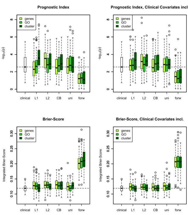
4.7.3 Prognostic Index . . . 42
4.7.4 Brier-Score . . . 42
4.7.5 Example for Calculating the Brier-Score . . . 44
Contents 2
5 Results 47
5.1 Descriptive Analysis of Data Sets . . . 48
5.2 Analysis Steps . . . 50
5.3 Exemplary Analysis: One Split into Training and Test Data . . . 55
5.4 Comparison of Selection Methods . . . 58
5.5 Analysis of Important GO Groups . . . 66
6 Discussion and Conclusion 69
Bibliography 73
Acknowledgements 77
Declaration 78
Abstract
An important application of high-dimensional gene expression measurements is the risk prediction and the interpretation of the variables in the resulting survival models.
A major problem in this context is the typically large number of genes compared to the number of observations (individuals). Feature selection procedures can generate predictive models with high prediction accuracy and at the same time low model complexity. However, interpretability of the resulting models is still limited due to little knowledge on many of the remaining selected genes. Thus, we summarize genes as gene groups defined by the hierarchically structured Gene Ontology (GO) and include these gene groups as covariates in the hazard regression models. Since expression profiles within GO groups are often heterogeneous, we present a new method to obtain subgroups with coherent patterns. We apply preclustering to genes within GO groups according to the correlation of their gene expression measurements.
We compare Cox models for modeling disease free survival times of breast cancer patients. Besides classical clinical covariates we consider genes, GO groups and preclustered GO groups as additional genomic covariates. Survival models with preclustered gene groups as covariates have improved prediction accuracy in long term survival compared to models built only with single genes or GO groups. We also provide an analysis of frequently chosen covariates and comparisons to models using only clinical information.
The preclustering information enables a more detailed analysis of the biological meaning of covariates selected in the final models. Compared to models built only with single genes there is additional functional information contained in the GO annotation, and compared to models using GO groups as covariates the preclustering yields coherent representative gene expression profiles. For evaluation of fitted survival models, we present prediction error curves revealing that models with preclustered gene groups have improved prediction performance compared to models built with single genes or GO groups.
1 Introduction 4
1 Introduction
Almost 10% of German women will develop invasive breast cancer over the course of their lifetime. In 2004, approximately 57 000new cases of breast cancer were diagnosed in women in Germany (Robert Koch Institut, 2010). Statistics for other countries, especially for the United States, are comparable (Ma and Huang, 2007). Despite major progresses in breast cancer treatment, the ability to predict the metastatic behavior of tumor remains limited.
In addition to well-known risk factors (cf. Robert Koch Institut, 2010) like drinking al- cohol, getting older, being overweight (increases risk for breast cancer after menopause) and not getting regular exercise, specific genes may have an influence on developing cancer and on patient’s survival times. According to Giersiepen et al. (2005) about5 to10% of breast cancers can be linked to gene mutations (abnormal changes) inherited from one’s mother or father. Mutations of the BRCA1 and BRCA2 genes are the most common. Women with these mutations have up to an 80% risk of developing breast cancer during their lifetime, and they are more likely to be diagnosed at a younger age (before menopause).
In the last 10 years cancer research has focused on gene expression experiments to detect genes that are responsible for the development of cancer and for its course over time. Thus, the prediction of cancer patient survival based on gene expression profiles is an important application of genome-wide expression data (Rosenwald et al., 2002;
van de Vijveret al., 2002; van ’t Veer et al., 2002).
In this thesis, our goal is to improve prediction accuracy and interpretability of high- dimensional models for prediction of survival outcomes, by combining gene expression data with prior biological knowledge on groups of genes.
Since 2001 numerous developments have appeared to outcome prediction for several kinds of cancer on the basis of gene expression experiments (Alizadeh et al., 2000;
Bair and Tibshirani, 2004; Beer et al., 2002; Khan et al., 2001; Rosenwald et al., 2002; Ramaswamy et al., 2003), with special focus on breast carcinoma (Sørlie et al., 2001; Rosenwald et al., 2002; van de Vijver et al., 2002; van ’t Veer et al., 2002;
Wang et al., 2005; West et al., 2001). Several of these studies reported considerable predictive success. They allow the discovery of new markers that open the way to more subject-specific treatments with greater efficacy and safety.
Clinical covariates like age, gender, blood pressure, tumor size and grade, as well as smoking and drinking history have been extensively used and shown to have satisfactory predictive power. They are usually easy to measure and of low dimensionality.
By uncovering the relationship between time to event and the tumor gene expres- sion profile, it is hoped to achieve more accurate prognoses and improved treatment strategies. Predicting the prognosis and metastatic potential of cancer at the time of discovery is a major challenge in current clinical research. Numerous recent studies searched for gene expression signatures that outperform traditionally used clinical parameters in outcome prediction (see e.g. Binder and Schumacher, 2008b). A substan- tial challenge in this context comes from the fact that the number of genomic variables p is usually much larger than the number of individuals n. The goal is to construct models that are complex enough to have high prediction accuracy but that are at the same time simple enough to allow biological interpretation. It is very difficult to select the most powerful genomic variables for prediction, as these may depend on each other in an unknown fashion.
Univariate approaches use single genes as covariates in survival time models, whereas multivariate models need a more elaborate framework. For statistical analysis, the Cox regression model (Cox, 1972) is a well-known method for modeling censored survival data. It can be used for identifying covariates that are significantly correlated with survival times. Due to the high-dimensional nature of microarray data we cannot obtain the parameter estimates directly with the Cox log partial likelihood approach. Techniques have been developed that result in shrunken and/or sparse models, i.e., models where only a small number of covariates is used. The classical
1 Introduction 6
ridge-regression (Hoerl and Kennard, 1970) and lasso-regression (Tibshirani, 1996, 1997) are particularly suitable. Efronet al.(2004) proposed a highly efficient procedure, called Least Angle Regression (LARS) for variable selection which can be used to perform variable selection with very large matrices. LARS can be modified to provide a solution for the lasso-procedure. Using the connection between LARS and lasso, Gui and Li (2005) proposed LARS-Cox for gene selection in high-dimension and low-sample settings. In this case and in boosting approaches (Bühlmann and Hothorn, 2007), it is avoided to discard covariates before model fitting. Parameter estimation and selection of covariates is performed simultaneously. This is implemented by imposing a penalty on the model parameters for estimation. The structure of this penalty is chosen such that most of the estimated parameters will be equal to zero, i.e., the value of the corresponding covariates does not influence predictions obtained from the fitted model.
Schumacher et al. (2007) developed techniques for extending a bootstrap approach for estimating prediction error curves (introduced by Gerds and Schumacher, 2007) to high-dimensional gene expression data with survival outcome.
An alternative method was developed by Binder and Schumacher (2008b). They proposed a boosting approach for high-dimensional Cox models (CoxBoost). The resulting model is sparse and thus it competes directly with the results from lasso- regression. Binder and Schumacher (2008b) applied the CoxBoost algorithm to gene expression data sets.
In addition, the combination of clinical data and gene expression data is a hot topic of research (cf. Boulesteix et al., 2008; Binder and Schumacher, 2008b). In order to integrate the clinical information and microarray data in survival models properly, it is a common approach to handle the clinical covariates as unpenalized mandatory variables (cf. Binder and Schumacher, 2008b; Bøvelstadet al., 2009). These approaches show that the combination of genomic and clinical information may also improve predictions.
For evaluating a fitted survival model, patients are often divided into subgroups according to their prognoses. Kaplan-Meier curves (Kaplan and Meier, 1958) are calculated for each group and compared with the log-rank test (see, e.g. Rosenwald et al., 2002). It is important that a comparison of groups is performed without the
individuals used for model fitting. Otherwise, results would be overoptimistic.
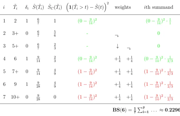
Graf et al. (1999) presented an adapted framework for the Brier-Score (Brier, 1950) for survival models with censored observations. At each time point, we compare the estimated probability of being event-free to the observed event-status. Analysis of the prognostic index (Bøvelstad et al., 2007) and the Brier-Score (Graf et al., 1999;
Schumacher et al., 2007) can be used to assess the predictive performance of the fitted models.
On the other hand, Haibe-Kainset al.(2008) showed in a comparative study of survival models for breast cancer prognostication based on microarray data that the most complex methods are not significantly better than the simplest one, a univariate model relying on a single proliferation gene. This result suggests that proliferation might be the most relevant biological process for breast cancer prognostication and that the loss of interpretability deriving from the use of overcomplex methods may be not sufficiently counterbalanced by an improvement of the quality of prediction of those who really need chemotherapy and benefit from it.
However, due to the large variability in survival times between cancer patients and the amount of genes on the microarrays unrelated to outcome, building accurate prediction models that are easy to interpret remains a challenge. In this thesis, we propose a new approach for improving performance and interpretability of prediction models by integrating gene expression data with prior biological knowledge. To raise the interpretability of prognostic models, we combine genes to gene groups (e.g. according to their biological processes) and use these groups as covariates in the survival models. The hierarchically ordered ’GO groups’ (Gene Ontology) are particularly suitable (Ashburner et al., 2000). The Gene Ontology (GO) project provides structured, controlled vocabularies and classifications according to molecular and cellular biology. Gene expression data can be analyzed by summarizing groups of individual gene expression profiles based on GO annotation information. The mean expression profile per group or the first principle component can then be used to identify interesting GO categories in relation to the experimental settings. Another platform is the KEGG data base (Kanehisa et al., 2004) that provides biological pathway information for genes and proteins.
1 Introduction 8
A problem when relating genes to groups is that the genes in each gene group may have different expression profiles: interesting subgroups may not be detected due to heterogeneous or anti-correlated expression profiles within one gene group. We propose to cluster the expression profiles of genes in every gene group to detect homogeneous subclasses within a GO group and preselect relevant clusters (preclustering). The Intra Cluster Correlation (ICC), a measure of cluster tightness, is applied to identify relevant clusters.
In a first step we compared high-dimensional survival models with genes and GO groups as covariates for different variable selection methods (Kammers and Rahnenführer, 2010). Based on this work Lang (2010) constructed in his diploma thesis different aggregation methods for genes within a gene group for high-dimensional data sets. It turned out that summarizing the expression values with the first principle component is the most promising aggregation method. This result is integrated in this thesis with an extensive model building and evaluation procedure. We show comparisons to clinical models and to combinations of genomic and clinical models with different types of evaluation measures as well as the analysis of frequently chosen covariates.
The main results of this thesis are already published in the peer-reviewed journal BMC Bioinformatics.
This thesis is organized as follows: Chapter 2 provides the biological background and introduces the data sets. Chapter 3 and 4 describe the statistical methodology for building prognostic models for high-dimensional data sets. Chapter 3 presents methods for summarizing gene expression measurements with a focus on preclustering and Chapter 4 introduces the survival framework including the Cox model for high- dimensional data and algorithms for fitting and evaluating it. Chapter 5 shows the main results for two breast cancer data sets. Chapter 6 discusses proper ways for placing the results within the context of recent studies and possibilities for extensions.
Concluding remarks are also given in this chapter.
2 Background and Data Sets
In Section 2.1 we present the biological and medical background of breast cancer including risk factors, types of therapy and relation to recent statistical research. In Section 2.2 and Section 2.3 we briefly introduce the microarray technology for gene expression experiments and the Gene Ontology database that provide supplementary information for many genes. Finally, in Section 2.4 we present two well-known breast cancer data sets that are used for all analysis steps in Chapter 5.
2.1 Breast Cancer
Breast cancer is a malignant tumor that starts in the cells of the breast. A malignant tumor is a group of cancer cells that can grow into (invade) surrounding tissues or spread (metastasize) to distant areas of the body. Usually breast cancer either begins in the cells of the lobules, which are the milk-producing glands, or the ducts, the passages that drain milk from the lobules to the nipple (see, e.g. Sariego, 2010). The disease occurs mostly in women, but men can be affected, too.
The size, stage, rate of growth, and other characteristics of the tumor determine the kinds of treatment. It may include surgery, drugs (hormonal therapy and chemother- apy), radiation and/or immunotherapy (Florescuet al., 2011). Surgical removal of the tumor provides the single largest benefit, with surgery alone being capable of producing a cure in many cases. To increase the disease-free survival, several chemotherapy regimens are commonly given in addition to surgery. Radiation is indicated especially after breast conserving surgery and substantially improves local relapse rates and in many circumstances also overall survival (Buchholz, 2009). Some breast cancers are
2 Background and Data Sets 10
sensitive to hormones such as estrogen and/or progesterone, which makes it possible to treat them by blocking the effects of these hormones.
Research has found several risk factors that may increase the chances of getting breast cancer. According to Robert Koch Institut (2010) an excerpt of risk factors is given by never giving birth, personal history of breast cancer or some non-cancerous breast diseases, family history of breast cancer (mother, sister, daughter), treatment with radiation therapy to the breast/chest, starting menopause at a later age, long-term use of hormone replacement therapy (estrogen and progesterone combined), drinking alcohol and getting older, being overweight (increases risk for breast cancer after menopause) and not getting regular exercise. In addition to these ’clinical’ factors, changes in the breast cancer-related genes BRCA1 or BRCA2 may also influence the susceptibility to breast cancer.
For lowering the risk of breast cancer the U.S. Preventive Services Task Force (2009) as well as Boyle and Levin (2008) suggest to be screened for breast cancer regularly and control the risk factors if possible.
Boyle and Levin (2008) point out that worldwide, breast cancer comprises 22.9% of all cancers (excluding non-melanoma skin cancers) in women. In 2008, breast cancer caused approximately 450 000 deaths worldwide corresponding to 13.7% of cancer deaths in women. Breast cancer is more than 100 times more common in women than breast cancer in men, although males tend to have poorer outcomes due to delays in diagnosis. Prognosis and survival rate vary greatly depending on cancer type, staging and treatment.
In the article of 2001, Cooper reviews the ways in which microarray technology (see Section 2.2) may be used in breast cancer research (Cooper, 2001). Today, the analysis of gene expression profiles of breast cancer patients and the combination of clinical and gene expression data is a hot topic of research and is very important for risk prediction in survival models (see, e.g., Bøvelstad et al., 2007, 2009; Boulesteixet al., 2008; Binder and Schumacher, 2008b; Binder et al., 2011).
2.2 Microarray Technology
Microarray technology represents a powerful functional genomics technology, which permits the expression profiling of thousands of genes in parallel (Schena et al., 1996) and is based on hybridisation of complementary nucleotide strands (DNA or RNA).
Microarray chips consist of thousands of DNA molecules (corresponding to different genes) that are immobilized and girded onto a support such as glass, silicon or nylon membrane. Each spot on the chip is representative for a certain gene or transcript.
The expression levels of all genes can be determined by isolating the total amount of mRNA, which is defined to be the transcriptome of the cell at the given time.
Fluorescently or radioactively labeled nucleotides (targets) that are complementary to the isolated mRNA are prepared and hybridized to the immobilized molecules.
Target molecules that did not bind to the immobilized molecules (probes) during the hybridization process are washed away. The amount of hybridized target molecules is proportional to the amount of isolated mRNA. The relative abundance of hybridized molecules on a defined array spot can be determined by measuring the fluorescent or radioactive signal.
Different types of DNA arrays are designed for mRNA profiling. These types differ by the type of probes that are immobilized on the chip (cDNA or synthetic oligonucleotides) and by the density (probes per square centimetre) of the array. The two basic microarrays variants areprobe cDNA (0.2to 5kb long) that is immobilized to a solid surface using robot spotting and synthetic DNA fragments (oligonucleotides, 20 to 80mer long) that are synthesized on-chip (Gene Chip, Affymetrix) or by conventional synthesis followed by on-chip immobilization. This high-density microarray type can carry up to 40 probes per transcript. Half of the probes are designed to perfectly match the nucleotide stretches of the gene, while the other half contains a mismatch (a faulty nucleotide) as a control to test for specificity of the hybridisation signal. Other microarray platforms, such as Illumina, use microscopic beads, instead of the large solid support.
2 Background and Data Sets 12
2.3 Gene Ontology Data Base
The Gene Ontology (GO) project is an international bioinformatics initiative to unify the representation of gene and gene product attributes across all species (Ashburner et al., 2000). This project provides a set of structured, controlled vocabularies for community use in annotating genes, gene products and sequences that are available from the GO web site http://www.geneontology.org. The ontologies have been extended and refined for several biological areas, and improvements to the structure of the ontologies have been implemented. The current ontologies of the GO project are biological process, molecular function, andcellular component.
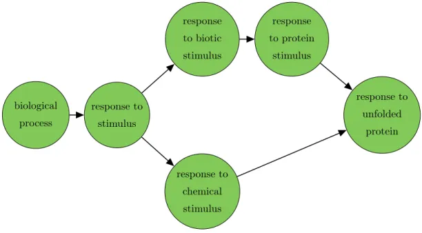
GO has a hierarchical structure that forms a directed acyclic graph (DAG). For such a graph we can use the notions of child and parent, where a child can have multiple parents. Every GO term (GO group) is represented by a node in this graph. The nodes are annotated with a set of genes. For an inner node of the GO graph, the corresponding set of genes also comprises all genes annotated to all children of this node. Figure 2.1 represents a part of this graph for the biological process ontology. The arrowhead indicates the direction of the relationship. Child nodes can have different relations to its parents note or its parents notes: a node may have apart of relationship to one node or anis arelationship to another. The biological process ontology includes terms that represent collections of processes as well as terms that represent a specific, entire process. The former mainly have is a relationships to their children, and the latter mainly have part of children that represent subprocesses.
response to biotic stimulus
response to protein
stimulus
biological process
response to stimulus
response to unfolded
protein
response to chemical stimulus
Figure 2.1: Exemplary part of the directed acyclic graph from Gene Ontology database.
2.4 Description of Data Sets
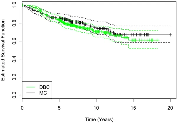
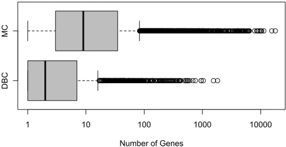
In this section we introduce two well-known breast cancer data sets that we use for the entire analysis (see Chapter 5): the Dutch breast cancer (DBC) data setand the Mainz cohort (MC) study. Both consist of genomic and clinical information as well as survival times and are therefore particularly suitable. The DBC data set is analyzed in several publications (see, e.g. Bøvelstad et al., 2007, 2009; Porzelius et al., 2009; van Wieringen et al., 2009) with models for time-to-event endpoints and thus our results are easy to compare to the already published ones. The MC study is a data set that is extensively used in our working group in cooperation with the Leibniz Research Centre for Working Environment and Human Factors (IfADo) at TU Dortmund University. The complete study data is well-known from its surgical origin to final data matrices. In addition, we want to highlight that there is no missing data in both data sets.
The Dutch breast cancer (DBC) data set is a subset of the original data set from the fresh-frozen-tissue bank of the Netherlands Cancer Institute with 24 885 gene expression measurements from n = 295 women with breast cancer. According
2 Background and Data Sets 14
to van de Vijveret al. (2002) and van Houwelingenet al. (2006) the following selection criteria were employed:
• the tumour was a primary invasive breast carcinoma of size less than 5cm in diameter,
• the age at diagnosis was 52 years or younger,
• the diagnosis was between 1984 and 1995, and
• there was no previous history of cancer, except non-melanoma skin cancer.
All patients had been treated by modified radical mastectomy or breast conserving surgery, including dissection of the axillary lymph nodes, followed by radiotherapy if indicated. Among the295patients,151were lymph node negative and144were lymph node positive. All tumors were profiled on cDNA arrays containing 24 885genes. After data pre-processing as proposed by van Houwelingen et al. (2006) the data set was reduced to a set of 4 919genes. The data, including gene expression measurements, clinical information and survival data for each patient, was obtained from the website https://www.msbi.nl/dnn/People/Houwelingen.aspx. Working with this reduced data set makes it easier to compare our results with previous publications (see, e.g.
Bøvelstad et al., 2007, 2009). Our analysis is performed with only1 876 genes, that are annotated to at least one GO group, according to the biological process ontology.
In total, there are 5 560 GO groups to which at least one of these genes is annotated.
The mean number of genes included in these GO groups is approximately 17 genes where 90% of all GO groups contain at most30 genes. For79 patients an event was observed. The clinical covariates are age, size, nodes and grade.
The Mainz cohort (MC) study consists of n = 200 node-negative breast cancer patients who were treated at the Department of Obstetrics and Gynecology of the Johannes Gutenberg University Mainz between the years 1988 and 1998 (Schmidt et al., 2008). All patients underwent surgery and did not receive any systemic therapy in the adjuvant setting. Gene expression profiling of the patients’ RNA was performed using the Affymetrix HG-U133A array, containing22 283probe sets, and the GeneChip System. These probe sets are identifiers for approximately 14 500 well-characterized human genes that can be used to explore human biology and disease processes. The
normalization of the raw data was done using RMA from the Bioconductor package affy. The raw .cel files are deposited at the NCBI GEO data repository with accession number GSE11121. For covariates in the survival models, 17 834 probe sets and 8 587 GO groups are available. The mean number of genes included in these GO groups is approximately 102 probe sets where90% of all GO groups contain at most146 probe sets and the number of observed events is 47. The clinical data covers age at diagnosis, tumor size and grade as well as the estrogen receptor status.
Probe sets can code for the same gene. We will not differentiate between probe sets and genes in the following and we call them genes.
3 Methods for Preclustering 16
3 Methods for Preclustering
In this chapter we present methods that search for correlated covariates and aggregation procedures that summarize these covariates. Partitioning around Medoids (PAM) is a clustering method that groups positively correlated variables according to their correlation matrix. This approach is introduced in Section 3.1 and followed by a permutation test for correlation in Section 3.2. This test is used for preselecting covariates within PAM-clustering and as an alternative for clustering when only two covariates are present. Further, we introduce simple aggregation methods for summarizing covariate information in Section 3.3. Finally, we present the principal component analysis (PCA) for multivariate dimension reduction in Section 3.4.
3.1 Partitioning Around Medoids Clustering
Partitioning around Medoids (PAM) (cf. Kaufman and Rousseeuw, 1995) is a clustering algorithm related to theK-means algorithm. Both algorithms are partitional (dividing the dataset into groups) and both attempt to minimize the squared error, the sum of squared distances of all data points to their respective cluster centers. PAM is more robust to noise and outliers compared to K-means because it minimizes the sum of pairwise dissimilarities instead of the sum of squared Euclidean distances.
Let X be a data matrix with n observations and p covariates. The PAM procedure is based on the search for K representative objects, the medoids ({m1, . . . , mK} ⊂ {1, . . . , p}), whose sum of average dissimilarity to all objects in the cluster is minimal.
Here, the objects are the covariates that should be clustered.
In order to find correlated subgroups, we first calculate the dissimilarity
dij = 1−Cor(xi, xj)
for all pairs (i, j) with values xi and xj (i, j = 1, . . . , p). In matrix notation, the dissimilarity matrix D, given by
D= 1−Cor (X) ∈Rp×p,
is generated by the data matrix X (X ∈ Rn×p). The distance between two column vectors is calculated via their correlation coefficient: if two column vectors are highly positive correlated, their distance is close to zero, if they are uncorrelated, their distance is one, if they are highly negative correlated, their distance is two. The correlation coefficient is calculated with the empirical Pearson’s correlation coefficient which is defined for two objects xand y with n values by
Cor (x, y) =
Pn
i=1(xi−x) (y¯ i−y)¯ q
Pn
i=1(xi−x)¯ 2·Pn
i=1(yi−y)¯ 2
, x¯= 1 n
n
X
i=1
xi, y¯= 1 n
n
X
i=1
yi.
LetC(C(i) : Np →NK) be a configuration function. The grouping of allpobjects inK homogeneous clusters is done with the function C that maps the object i(i= 1, . . . , p) to cluster k (k∈1, . . . , K) according to the smallest dissimilarity to the medoids
C(i) = argmin
1≤k≤K
dimk. (3.1)
To evaluate a solution with given medoids and the resulting configuration of all objects, we calculate the sum of intra-cluster-dissimilarities (often referred to as cost-function):
H(m1, . . . , mK) =
K
X
k=1
X
C(i)=k
dimk. (3.2)
The PAM optimization problem is the minimization of equation (3.2) regarding to the choice of the medoids and considering the mapping rule (3.1).
3 Methods for Preclustering 18
The two following steps are carried out iteratively until convergence, starting with K randomly selected objects as initial solution (m1, . . . , mK):
1. Build: Select sequentially K initial clusters and assign each gene to its closest medoid.
2. Swap: For each medoid mk and all non-medoid objects θ, swap mk and θ, then calculate the homogeneity measure given in equation (3.2) and finally select the configuration of medoids with the lowest cost.
Note that we have to test (K ·(p−K)) swaps in eachSwap step.
The number of clusters K for the PAM algorithm has to be chosen in advance. There are several techniques that provide adequate measures or graphical representation of how well each object lies within its cluster, e.g. the average silhouette width (cf.
Rousseeuw, 1987). To find tight clusters of highly correlated objects, De Haan et al.
(2010) suggest using the Intra Cluster Correlation. For each possible number of clustersK, the normalized sums of all elements of the lower triangle of the correlation matrix are computed for each cluster. Afterwards, the arithmetic mean over all clusters is calculated. Thus, the optimal number of clusters KICC according to this method is given by
KICC = argmax
K=1,...,n−1
1 K
K
X
k=1
2 nk(nk−1)
nk
X
ik,jk=1
jk>ik
Cor (xik, xjk)
,
with object indices ik andjk containing nk single objects in cluster k. If the term in the round brackets consists of only one object, the term is zero by definition. The maximum meanKICC among the K = 2, . . . ,(N −1)possible cluster configurations corresponds to the optimal number of clusters within the given data set. Alternative calculations for the optimal number of clusters are e.g. provided in Hastie et al. (2009) and in Kaufman and Rousseeuw (1995).
3.2 Permutation Test for Correlation
A permutation test is a statistical test in which the distribution of the test statistic under the null hypothesis is obtained by calculating all possible values of the test statistic under rearrangements of the labels of the observed data points. Let Ψ be a (n×n)permutation matrix that has exactly one entryonein each row and each column andzeros elsewhere. Each such matrix represents a specific permutation of n elements and, when used to multiply with a vectorx∈Rn, can produce that permutation within the vector. For each of the permuted vectors, we can calculate the test statistic and the ranking of the observed test statistic among the permuted test statistics provides a p-value.
In our context, we look at a group withp objects (e.g. gene expression measurements) and investigate if object i has a positive correlation with at least one object of the group. We can formulate the following hypotheses:
H0: ith object has no correlation with another object
H1: ith object has a correlation with at least one other object.
The maximum correlation C0 ∈R between objecti and all other (p−1) objects can be calculated with
C0 = max
j∈{1,...,p}\i
Cor (xi, xj) , (3.3) in which xj (j = 1, . . . , p) represents then-dimensional vector of object j. In the case p= 2, the maximum correlation is reduced to Cor (x1, x2).
The vector Cp ∈RNp represents theNp maximum correlations after applying Np times a permutations-matrix Ψ onxi:
Cp=
max
j∈{1,...,p}\i
Cor (Ψ·xi, xj)
1,...,Np
.
According to Buening and Trenkler (1994) we can calculate the p-value p(i) for object i with
p(i) = 1−
1,0, . . . ,0
·Rg
C0, Cp>>
Np+ 1 , (3.4)
3 Methods for Preclustering 20
where Rg(·)is the rank statistic. IfC0 has a high rank, the ratio in (3.4) is close to one and thus the p-value p(i) is close to zero. For p-values smaller than a given significance level α, we have to reject the null hypothesis.
It is important to note that the number of permutationsNp should be large. Common values are in the range of 105 or greater, depending on the size of the data set.
3.3 Simple Aggregation Methods
In this section we present simple aggregation methods for summarizing information of several covariates to one single representative covariate. There are a number of methods for summarizing groups of covariates. Starting with a data matrix X ∈Rp×n, we are looking for a dimension reducing function:
f :Rp×n →Rn, f(x1, . . . , xp) = y, x1, . . . , xp, y ∈Rn (3.5)
where the generated variable y should be a representative vector for the group of covariates x1, . . . , xp and the loss of information should be minimized.
A simple possibility for summarizing a set of covariates is given by standard measures of location. Component wise computation of the arithmetic mean
¯ x= 1
n
n
X
i=1
xi
and of q-quantiles
˜ xq=
xdnqe, if nq6∈N
1
2 x(nq)+x(nq+1)
, if nq∈N
of the data matrix X ∈Rp×n could be performed. The median x˜0.5 corresponds the 0.5-quantile.
Another possibility to summarize covariate information is directly provided by results of the PAM-clustering approach: medoids of clusters are particularly suitable to represent groups and no further aggregation has to be performed.
3.4 Principle Component Analysis
Correlation structures within high-dimensional data sets could be interpreted as redundant information. Principal components analysis (PCA) is a method that reduces data dimensionality by finding a new set of covariates, smaller than the original set of covariates, that nonetheless retains most of the sample’s information, i.e. the variation present in the data set, given by the correlations between the original covariates. The new covariates, called principal components (PCs), are uncorrelated, and are ordered by the fraction of the total information each retains. As such, it is suitable for data sets in multiple dimensions, such as large experiments in gene expression. PCA on genes will find relevant components, or patterns, across gene expression data.
Mathematically, PCA is defined as an orthogonal linear transformation that transforms the data to a new coordinate system such that the greatest variance by any projection of the data comes to lie on the first coordinate (called the first principal component), the second greatest variance on the second coordinate, and so on.
The PCA is in general computed by determining the eigenvectors and eigenvalues of the covariance matrix. To calculate the covariance matrix from a data set given by a (p×n) matrix X, we first center the data by subtracting the mean of each sample vector. Considering the columns of the centered data matrix X as the sample vectors, we can write the covariance matrix of the samples Cn as:
Cn= 1 nXX>.
If we are interested in the covariance matrix for then p-dimensional covariates (i.e. gene expression measurements), we first center the data for each covariate. The covariance matrix Cp is then given by
Cp = 1 pX>X.
Often the scale factors n1 and 1p are included in the matrix and the covariance matrices are simply written asXX>andX>X, respectively. The eigenvectors of the covariance matrix are the axes of maximal variance. Since we are only interested in the PCA for the p-dimensional covariates we present a solution for X>X in the following.
3 Methods for Preclustering 22
With the help of singular value decomposition (SVD) (cf. Wall et al., 2003) the factorization of an arbitrary real-valued (p×n) matrix X with rank r is obtained by
X =UΣV>, U ∈Rp×n, Σ∈Rn×n, V ∈Rn×n. (3.6)
Here U is a (p×n) orthogonal matrix (U>U =Idp) whose columns uk are called the left singular vectorsand V is a(p×p)orthogonal matrix (V>V =Idp) whose columns vk are called the right singular vectors. The elements of the (n×n)matrix Σ are only nonzero on the diagonal, and are called the singular values. The firstr singular values of Σ = diag (σ1, . . . , σn) are sorted in decreasing orderσ1 ≥σ2 ≥. . .≥ σr > σr+1 = . . .=σn = 0.
The advantage of the SVD is that there are a number of algorithms for computing the SVD. One method is to compute V and S by diagonalizing X>X:
X>X=VΣ2V>
and then to calculate U by ignoring the (r+ 1), . . . , ncolumns of V with σk= 0
U =XVΣ−1.
The SVD and PCA are closely related. As mentioned before, the covariance matrix for X isX>X. With the help of the SVD, we can write
X>X = (UΣV>)(UΣV>)> =UΣV>VΣU> =UΣ2U>
using the fact that V is orthogonal, thus V> = V−1. Further, U can be calculated as the eigenvectors of X>X. The diagonal of Σ contains the square roots of the eigenvalues of the covariance matrix and the columns of U form the eigenvectors.
An important result of the SVD of a matrix X is that
X(l) =
l
X
k=1
ukσkvk>
is theclosestrankl matrix toX (closestmeans thatX(l) minimizes the sum of squares of the differences P
ij
xij −x(l)ij 2
of the elements of X and X(l)).
For dimension reduction, we determine in advance the number of covariates p0 ≤ p which should be selected. In most cases the number of selected PCs is due to the proportion of variance accounted, to which the singular values are proportional. Timm (2002) points out that the explained cumulated proportion of the variance in the data
α for the first p0 principal components is
α = Pp0
j=1σ2j Pp
j=1σ2j.
If we only consider the first principle component of the data matrix X the aggregated matrixX(l) is reduced to a single vector that represents all pcovariates of the observed data matrix X.
4 Methods in Survival Analysis 24
4 Methods in Survival Analysis
Survival analysis involves the modeling of time to event data where the response is often referred to as failure time, survival time, or event time. We focus on applying the techniques to biological and medical applications, i.e. the death or progression of cancer patients is the event of interest. A common feature in these data is that censoring is present when we have some information about an individual’s event time, but we do not know the exact event time. For the analysis methods we assume that the censoring mechanism is independent of the survival mechanism.
In this thesis, we will focus on right-censoring, where all that is known is that the individual is still event-free at a given time. There are a lot of reasons why right- censoring may occur. A typical censoring circumstance is that an individual does not experience the event before the study ends, an individual is lost to follow-up during the study period or an individual withdraws from the study. Censoring rates of more than 50% are not unusual in cancer data sets and a main challenge of survival analysis is the integration of the censoring information in the statistical methodology instead of deleting this data.
In this chapter, we introduce the basis functions, the survival function, and the hazard rate, for modeling survival data in Section 4.1. Basic estimates of the survival function and the hazard rate and the corresponding standard errors are discussed in Section 4.2 and Section 4.3. In Section 4.4, we present the log-rank test for detecting differences in survival in a two sample setting. Including covariate information (clinical and genomic variables) of the individuals leads to more detailed survival models. We consider Cox’s proportional hazards model (Cox model), introduced by Cox (1972), in Section 4.5 with a detailed description in the high-dimensional setting in Section 4.6, including a model selection and evaluation procedure. Since most methods for dimension reduction
or shrinkage require the selection of a tuning parameter that determines the amount of shrinkage, we describe how to choose the optimal tuning parameter for the presented methods.
4.1 Introduction to Survival Analysis
Let T be a positive random variable which represents the time from a well-defined starting point t = 0 to an event of interest with density f(t) and corresponding distribution function F(t). We define the survival function (the probability of being event-free up to time t) by
S(t) =P (T > t).
According to the relationship to the distribution function F (t) = 1−S(t), it is easy to see that the survival functionS(t) is right-continuous and monotonically decreasing with limits S(t) = 0 for t→ ∞ and S(t) = 1for t →0. In Section 4.2, we introduce an estimator for the survival function.
The hazard rate (function) λ(t), also called risk functionor conditional failure rate, is the chance that an individual experiences an event in the next instant time, conditional on survival until time t:
λ(t) = lim
h↓0
P (t≤T < t+h|T > t)
h , λ(t)≥0∀t ∈[0,∞].
If T is a continuous random variable, the relationship between the survival function and the hazard rate is given by
λ(t) = lim
h↓0
P (t≤T < t+h) h
1 P (T > t)
= f(t) S(t) =
∂
∂tF(t)
S(t) = −∂t∂S(t)
S(t) =−∂
∂tln (S(t)).
A related quantitiy is the cumulative hazard function Λ(t), defined by
Λ(t) = Z t
0
λ(u) du= Z t
0
f(u) S(u)du=
Z t 0
δ δuF(u)
S(u) du=− Z t
0 δ δuS(u)
S(u) du=−lnS(t).
4 Methods in Survival Analysis 26
A well-established estimator for the cumulative hazard function is the Nelson-Aalen estimator that is introduced in Section 4.3.
4.2 Kaplan-Meier Estimator
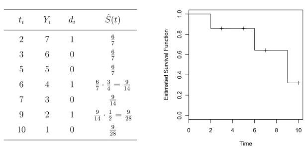
The standard nonparametric estimator for the survival function S(t) introduced by Kaplan and Meier (1958) is called Kaplan-Meier estimator or Product-Limit estimator.
To allow for possible ties in the data, we considerDdistinct event timesti(i= 1, . . . , D) with ti < ti+1 with di events at time ti. Note that censoring is not an event. Let Yi be the number of individuals who are at risk at time ti, e.g. the number of individuals who are alive at time ti or experienced the event of interest at ti. The Kaplan-Meier estimator Sˆ(t) is defined (for all values oft in the range where there is data) by:
Sˆ(t) =
1, t < t1
Q
ti≤t
1− Ydi
i
, t ≥t1.
According to Klein and Moeschberger (2003, Chapter 4.2)S(t)ˆ is a consistent estimator of the survival function S(t). There are analogous relations between the estimates as between the survival function and the distribution function. The Kaplan-Meier estimator is a monotone decreasing step function with jumps at the observed event times and is well defined for all time points less than the largest observation. If the largest time point is an event, the survival curve is zero beyond this point. If the largest point is censored, the value S(t)ˆ beyond this point is undetermined. There is no information when the last survivor would have died if the survivor had not been censored.
The standard error of the Kaplan-Meier estimator S(t)ˆ is estimated by Greenwood’s formula (see Klein and Moeschberger, 2003, Chapter 4.2):
SE S(t)ˆ
= ˆS(t)· s
X
ti<t
di
Yi(Yi−di).
The standard error is especially required for the calculation of pointwise (1−α)confi- dence intervals, given by
hS(t)ˆ ±u1−α/2SE S(t)ˆ
i .
Here uα is the α-quantile of a standard normal distribution N(0,1).
For testing differences in survival of two or more groups, the log-rank test is introduced in Section 4.4.
4.3 Nelson-Aalen Estimator
The Kaplan-Meier estimator can also be used to estimate the cumulative hazard func- tion Λ(t) =−lnS(t); the estimation is obtained by Λ(t) =ˆ −ln ˆS(t). An alternative estimator of the cumulative hazard rateΛ(t)was suggested by Nelson (1972) and Aalen (1978). With the notation of Section 4.2 and the assumption that all time points are
distinct, the Nelson-Aalen estimatorof the cumulative hazard rate Λ(t)is given by Λ(t) =ˆ X
ti≤t
λ(tˆ i) = X
ti≤t
di Yi.
According to the connection between the survival function S(t) and the cumulative hazard rate Λ(t),
S(t) = expˆ
−Λ(t)ˆ
= exp −X
ti≤t
di Yi
!
is an alternative estimator for the survival function.
4 Methods in Survival Analysis 28
4.4 Log-rank Test
In this section, we focus on hypothesis tests that are based on comparing the Nelson- Aalen estimates for two or more groups. In the survival context the most frequently used test is the log-rank test that compares the differences in hazard rates over time.
According to Klein and Moeschberger (2003, Chapter 7.3) we test the following set of hypotheses:
H0: λ1(t) = λ2(t) = . . .=λK(t), ∀t≤τ,vs.
H1: ∃i, j ∈1, . . . , K, ∃t ≤τ: λi(t)6=λj(t).
Here τ is the largest time at which all groups have at least one individual at risk. The test statistic is now constructed with the Nelson-Aalen estimator (see Section 4.3).
We consider distinct event times of the pooled population with the notation from Section 4.2. At timeti we observedij events in thejth population out ofYij individuals at risk. The test statistic is based on a weighted comparison of the estimated hazard rate of the jth population and the estimated pooled hazard rate. Let Wj(ti) be a positive weight function with the property Wj(ti) = 0 whenever Yij = 0. The general test for the jth group is based on the statistics
Zj(τ) =
D
X
i=1
Wj(ti) dij
Yij − di Yi
, di =
K
X
j=1
dij, Yi =
K
X
j=1
Yij, j ∈1, . . . , K.
By the specific choice of the weight function the influence of early and late observations can be controlled. The log-rank test is defined by Wj(ti) =YijW(ti) with W(ti)≡1.
Thus, the rewritten test statistics
Zj(τ) =
D
X
i=1
W(ti)
dij −Yijdi Yi
, j ∈1, . . . , K
show that all event times have equal weights. The entriesσˆjg of the covariance matrixΣˆ for the log-rank test are estimated by
ˆ
σjj2 := Var (Zj(τ)) =
D
X
i=1
Yij Yi
1− Yij Yi
Yi−di Yi−1
di, j = 1, . . . , K, and
ˆ
σ2jg := Cov (Zj(τ), Zg(τ)) =
D
X
i=1
Yij Yi
Yig Yi
Yi−di Yi−1
di, j, g= 1, . . . , K, j6=g.
The test statistic is given by
χ2LR = (Zi(τ), . . . , ZK−1(τ)) ˆΣ−1(Zi(τ), . . . , ZK−1(τ))>.
If the null hypothesis is true, this statistic follows aχ2-distribution with(K−1)-degrees of freedom. The null hypothesis is rejected at a given α level ifχ2LR is larger than the (1−α)-quantile of this distribution.
4.5 Cox Proportional Hazard Model
In addition to the event times there are often covariates observed that might have impact on survival. In order to cope with right-censored survival data we use the Cox model, also referred to as the proportional hazards regression model (see Cox, 1972).
First, we introduce the notation. As before, let T denote the time to event with density f(t), distribution functionF(t) and corresponding survival functionS(t). We also consider the situation of possibly right-censored time to event data. Let C be the positive random variable that represents the censoring times. A common assumption in survival context (see, e.g., Gerds and Schumacher, 2006) is that T and C are independent. We assume that C is distributed according to SC(t) = P(C > t) = 1−FC(t).
In the usual setup of survival data, we observe for each of the i= 1, . . . , nindividuals the triple( ˜Ti, δi, Zi), where T˜i = min(Ti, Ci)is the minimum of the event times Ti and the censoring times Ci. In addition, the censoring information is represented by the (non-censoring-)indicator δi =I{Ti≤Ci}. δi is equal to 1 if T˜i is a true event time and
4 Methods in Survival Analysis 30
equal to 0 if it is right-censored. For each individual i, the covariate information is given by a p-dimensional vector of covariates Zi = (Zi1, . . . , Zip)>.
Cox (1972) suggested that the risk of an event at time t for an individual i with given covariate vector Zi = (Zi1, . . . , Zip)> is modeled as
λ(t |Z =Zi) =λ0(t) exp (β>Zi), (4.1)
where λ0(·)is an arbitrary baseline hazard function and β = (β1, . . . , βp)> a vector of regression coefficients. The value of β>Zi is calledprognostic index (PI) or risk score of individual i. In other words: PI is the sum of the covariate values of a particular individual, weighted by the corresponding (estimated) regression coefficients.
As mentioned before, the Cox model is often called a proportional hazards model and assumes that for two covariate values Z1 and Z2 the ratio of their hazard rates is constant over time:
λ(t|Z1)
λ(t|Z2) = λ0(t) exp β>Z1
λ0(t) exp (β>Z2) = exp β>(Z1−Z2)
= const.
In the classical setting withn > p, the regression coefficients are estimated by Maximum Likelihood Estimation (MLE). We suppose that there are no ties between the ordered event times t1 < t2 < . . . < tD. The likelihood is only calculated for the event times.
The risk set R(ti) at time ti (that also includes the censoring times) is defined by
R(ti) = {j: tj ≥ti},
as the set of all individuals who have not yet failed nor been censored. The partial likelihood can be written as
L(β) =
D
Y
i=1
Li
!
=
D
Y
i=1
exp (Pp
k=1βkZik) P
j∈R(ti)exp (Pp
k=1βkZjk). (4.2) Here, the numerator of the likelihood depends only on information from individuals having an event, whereas the denominator consists of information of all individuals having not yet experienced the event or who may be censored later. Note that Cox’s
partial likelihood estimation method ignores the actual event times; it takes the ordering of events into account, but not their explicit values. For this reason the likelihood is referred to be partial.
Maximizing the partial likelihood is equivalent to maximizing the log partial likelihood
LL(β) = ln
D
Y
i=1
Li
!
=
D
X
i=1
ln (Li)
=
D
X
i=1 p
X
k=1
βkZik−
D
X
i=1
ln
X
j∈R(ti)
exp
p
X
k=1
βkZjk
!
, (4.3)
which corresponds to solving the following system of equations: Uk(β) := ∂β∂
kLL(β) = 0 for all k = 1, . . . , p. The vector U(β) with components Uk is called efficient score vector.
The estimation of the baseline hazard rate λ0(t) is performed after the estimation of the regression coefficients β1, . . . , βp with the Breslow estimator (see Klein and Moeschberger, 2003, Chapter 8.8)
λˆ0(t) =X
ti≤t
di P
j∈R(ti)exp
βˆ>Zj
.
There are several suggestions for constructing the partial likelihood when ties among the event times are present. A widely used adaption of the likelihood was suggested by Efron (1977):
LE(β) =
D
Y
i=1
exp β>
P
j∈DiZj Qdi
j=1
hP
k∈R(ti)exp (β>Zk)− j−1d
i
P
k∈Diexp (β>Zk)i.
Heredi is the number of events at timeti andDi the set of individuals who experience an event at time ti. Even though the partial likelihood (equation 4.2) and its adapted version by Efron show similar results in practice, we utilize Efron’s version for our calculations.
Maximizing Cox’s partial likelihood does not work for p n and some dimension
4 Methods in Survival Analysis 32
reduction or regularization methods must be used. The lasso- and ridge-regression are possibilities to jointly optimize over the parameters (see Section 4.6.1).
4.5.1 Hypothesis Testing
There are three main tests for hypotheses for the regression coefficientsβ = (β1, . . . , βp)>. Let βˆ = ( ˆβ1, . . . ,βˆp)> denote the maximum likelihood estimate of β. All three sta- tistical tests have as null hypothesis that the set of regression parameters β is equal to some particular value β0 (H0: β = β0 vs. H1: β 6= β0). For testing whether the regression coefficients have an effect of individuals’ risk to die or not, we chooseβ0 = 0.
We start with presenting the (efficient) score test, followed by the Wald test and the likelihood-ratio test. Note that the Wald test and the likelihood-ratio test are asymptotically equivalent.
4.5.2 Score Test
The score test is the most powerful test when the true value of β is close to β0. The main advantage of the score test is that it does not require an estimate of the information under the alternative hypothesis or unconstrained maximum likelihood.
This makes testing feasible when the unconstrained maximum likelihood estimate is a boundary point in the parameter space. LetU(β) = (U1(β), . . . , Up(β))be the efficient score vector defined in Section 4.5 and I(β) the (p×p) information matrix evaluated at β:
I(β) =
− ∂2
∂βj∂βkLL(β)
p×p
, j, k= 1, . . . , p.
Here, LL(β) is the log partial likelihood (see Section 4.5) evaluated at β. According to Klein and Moeschberger (2003, Chapter 8.3), U(β) is asymptotically p-variate normal with mean vector 0 and covariance matrix I−1(β) whenH0 is true. The score test for H0: β=β0 is given by
χ2SC =U(β0)>I−1(β0)U(β0)
having a χ2-distribution with p degrees of freedom under H0. We reject the null hypothesis at a significance levelαif χ2SC > χ2p,1−α. Here, χ2p,1−α is the(1−α)-quantile of the χ2-distribution with p degrees of freedom.
4.5.3 Wald Test
The Wald test (first suggested by Wald, 1943) compares the maximum likelihood estimate βˆ of the parameter vector of interest β with the proposed value β0, with the assumption that the difference between the two will be approximately normal.
Typically the square of the difference weighted with the covariance matrix I−1(β) is compared to a chi-squared distribution. With the notation from Section 4.5.2, the Wald test for the global hypothesis H0: β =β0 is defined by
χ2W = ( ˆβ−β0)>I−1( ˆβ)( ˆβ−β0)
and has a χ2-distribution with pdegrees of freedom if H0 is true.
4.5.4 Likelihood-ratio Test
A likelihood ratio test is used to compare the fit of two models: the null model using β0 and the alternative model using the parameter estimateβ. The test is based on theˆ likelihood ratio, which expresses how many times more likely the data are under one model than under the other. This likelihood ratio, or equivalently its logarithm, can then be used to compute a p-value to decide whether to reject the null model in favor of the alternative model. Both competing models, the null model and the alternative model, are fitted separately to the data and the log-likelihood is recorded. The test statistic is twice the difference of these log-likelihoods:
χ2LR = 2
LL( ˆβ)−LL(β0)
which has a χ2-distribution withp degrees of freedom under H0.
4 Methods in Survival Analysis 34
4.5.5 Local Test
In cases of variable selection, we are also interested in testing a hypothesis for single components βˆi of β. These tests are often calledˆ local tests and are presented in detail in Klein and Moeschberger (2003, Chapter 8.5). Exemplary, we present the Wald local test that we utilize e.g. for forward selection described in Section 4.6.3. In the univariate case, the Wald test statistic for the two-sided test with β0 ∈R
H0: ˆβi =β0 vs. H1: ˆβi 6=β0
is given by
W =
βˆi−β0 SE
βˆi,
which is compared to a normal distribution. The standard error SE βˆi
is derived by the corresponding value of the information matrix of the maximum likelihood estimate, i.e. square root of the ith diagonal element of I−1(β). Typically the square W is compared to a chi-squared distribution.